Spatial Prediction of Future Flood Risk: An Approach to the Effects of Climate Change


Abstract
1. Introduction
2. Materials and Methods
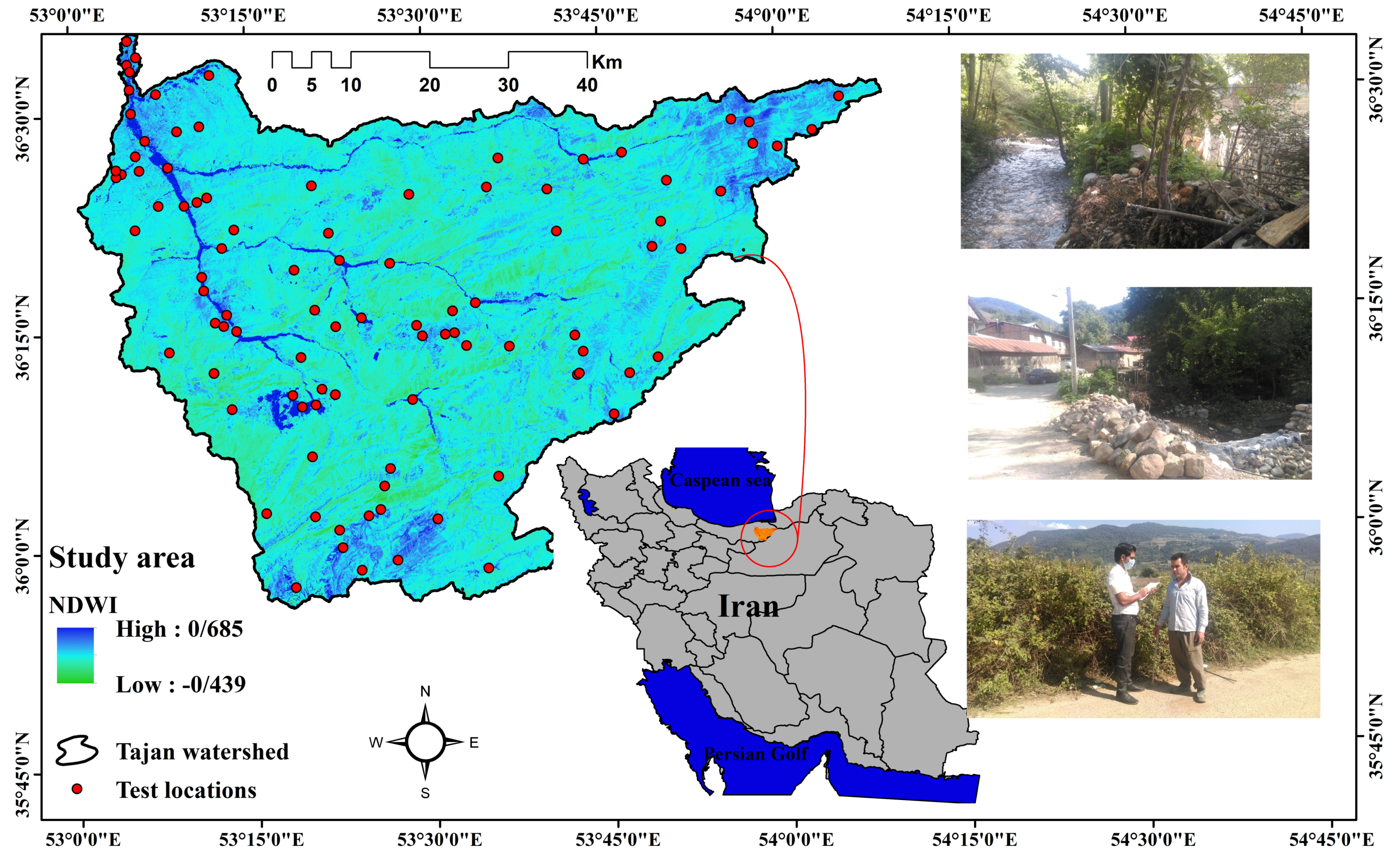
2.1. Description of the Study Area
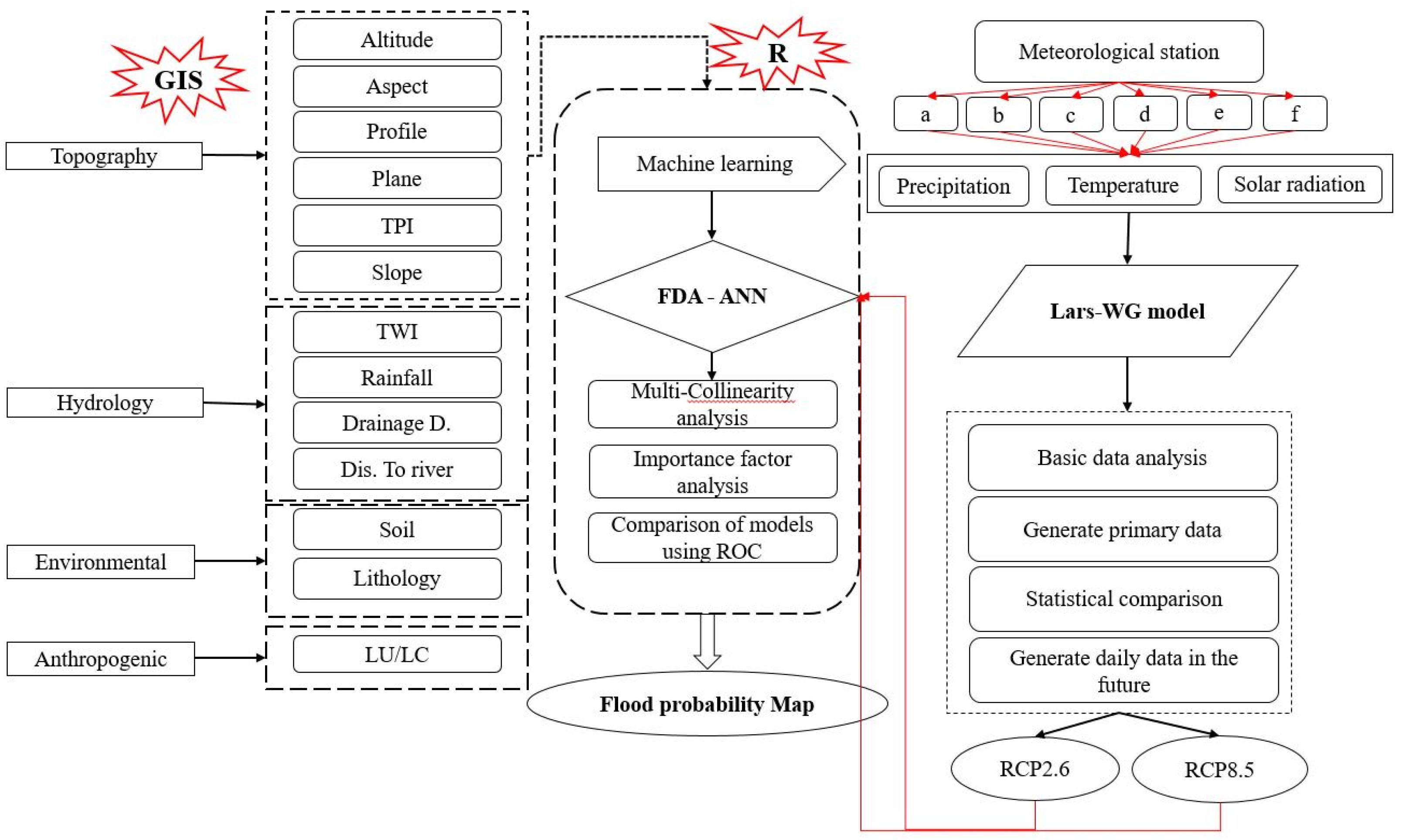
2.2. Methods
2.2.1. Flood Inventory Map
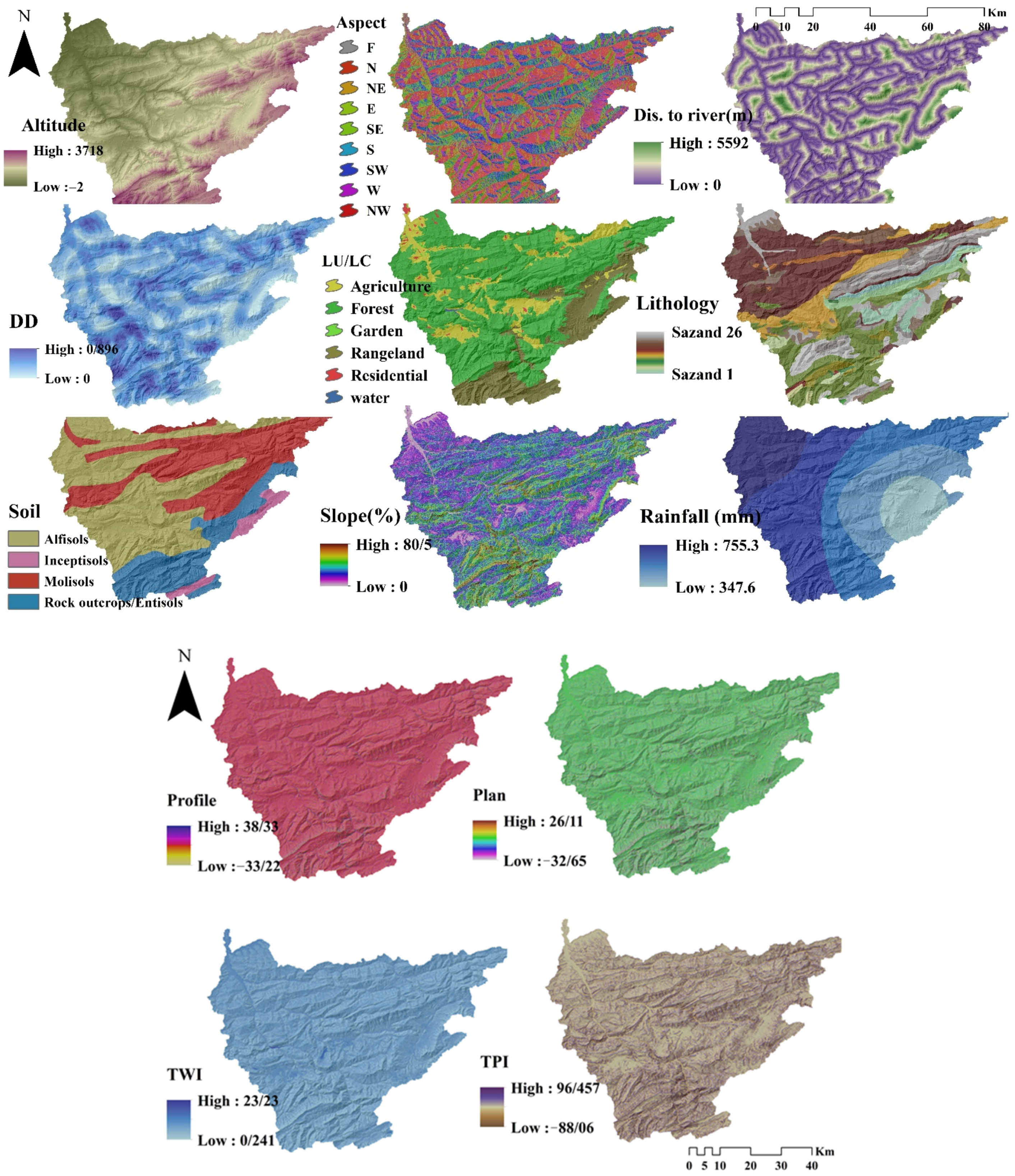
2.2.2. Flood Conditioning Factors
Topographical Conditioning Factors
Hydrological Conditioning Factors
Environmental Conditioning Factors
2.3. Description of the Data Mining Model
2.3.1. Flexible Discrimination Analysis (FDA)
- Lots of data, many predictors: LDA under fits (restricts to linear boundaries)
- Many correlated predictors: LDA (noisy/wiggly coefficients)
- Dimension reduction limited by the number of classes
2.3.2. Artificial Neural Network (ANN)
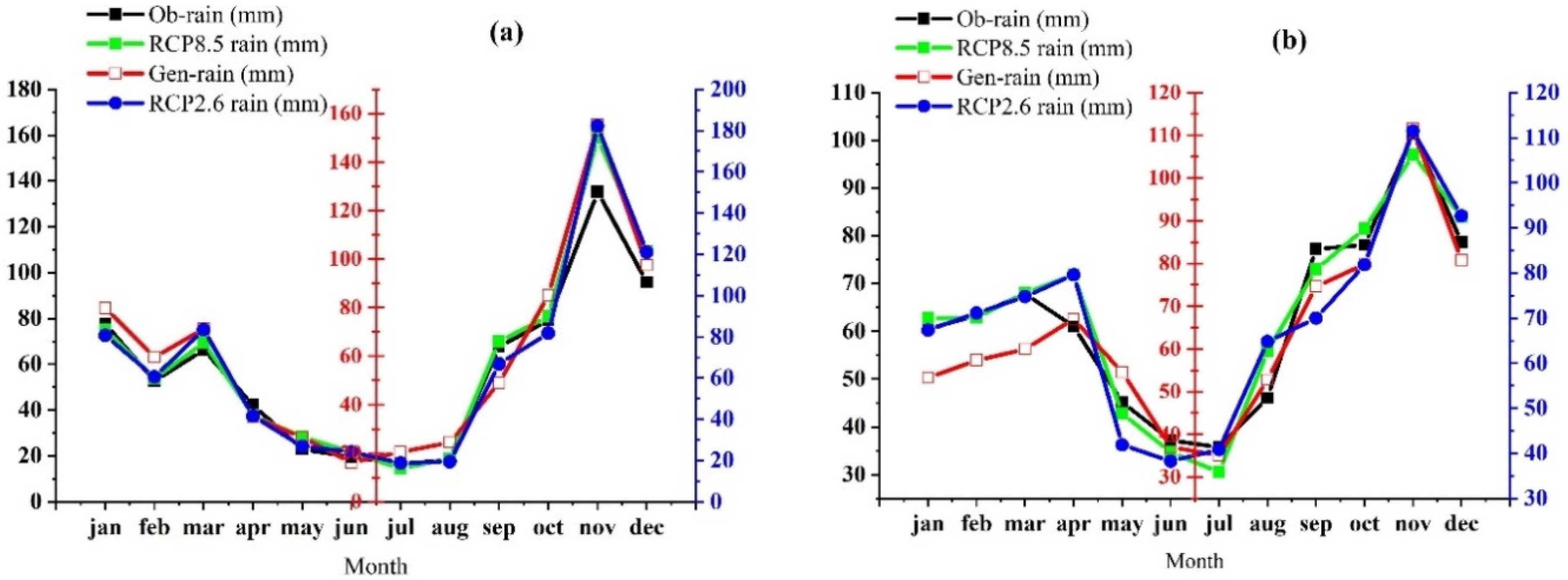
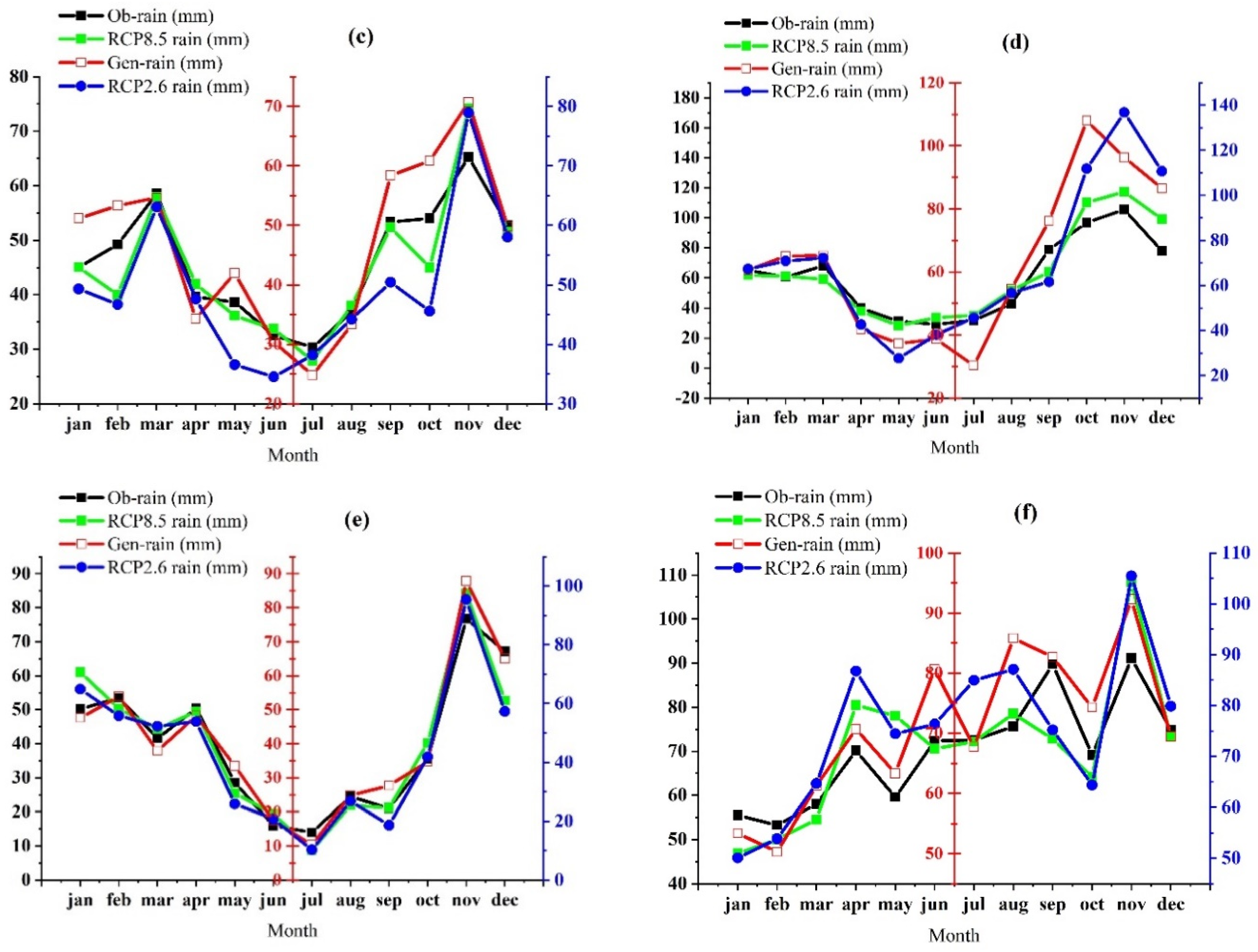
2.4. Predicting Climate Change
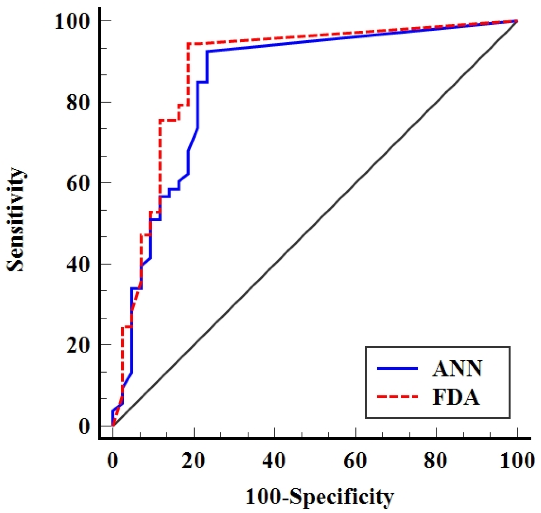
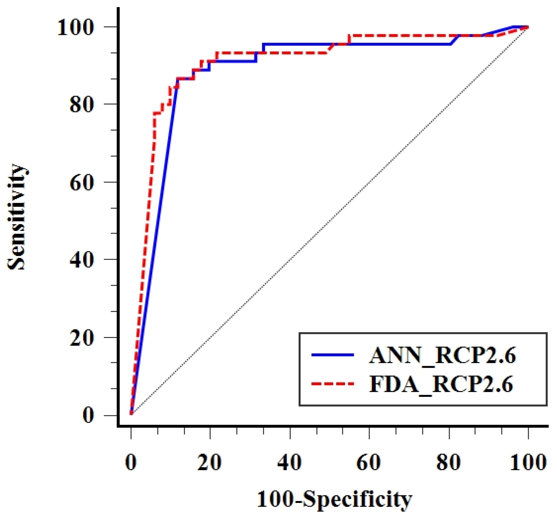
2.5. Receiver Operating Characteristic (ROC)
3. Results
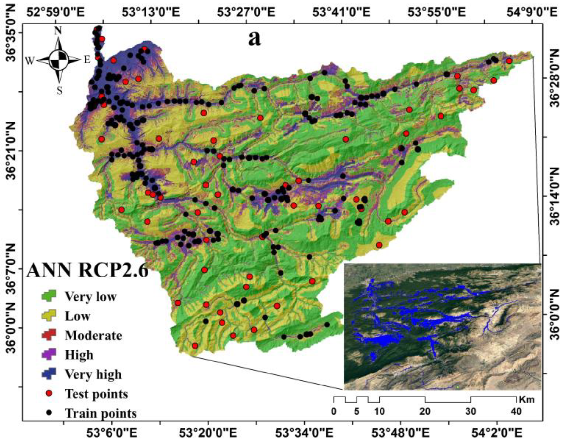
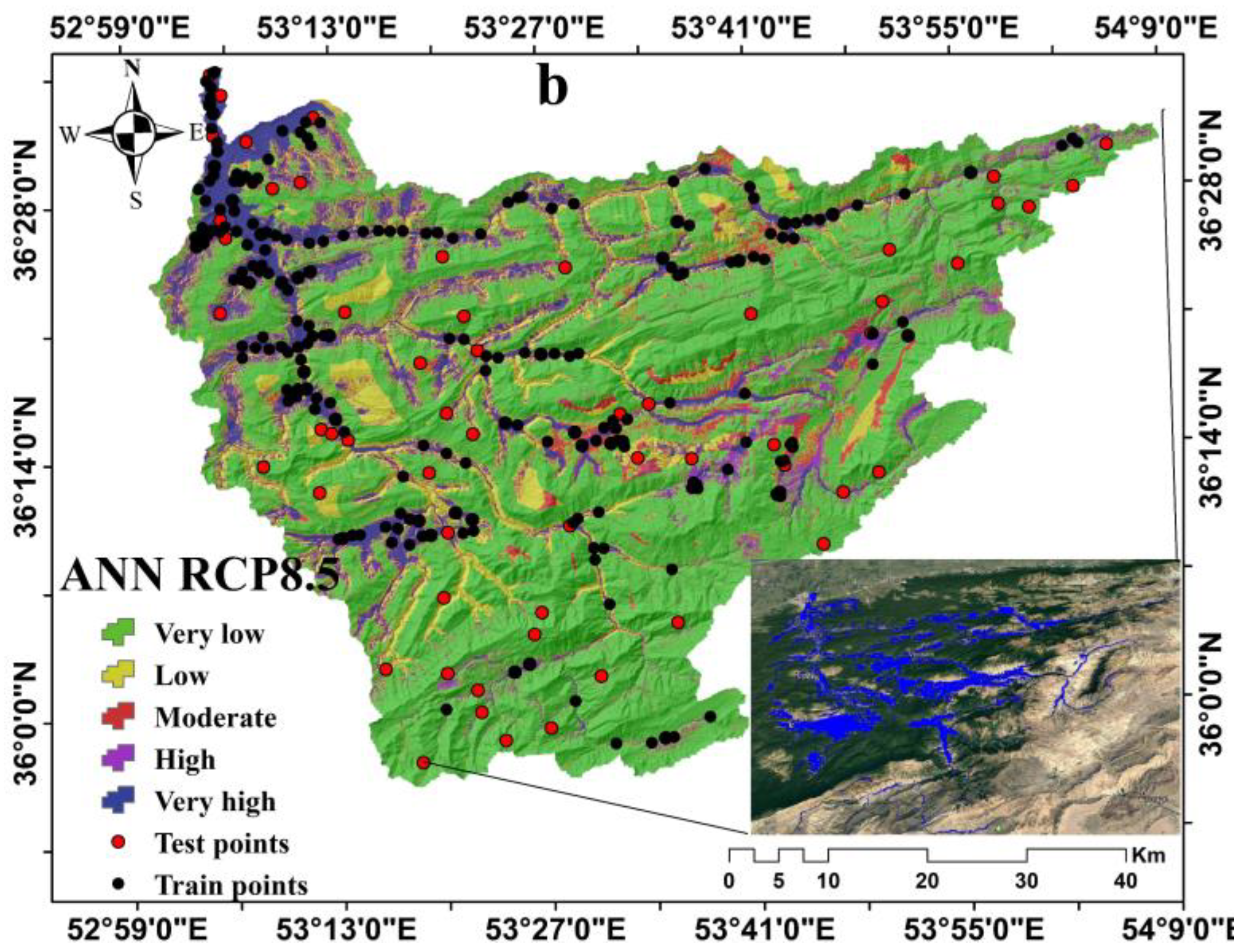
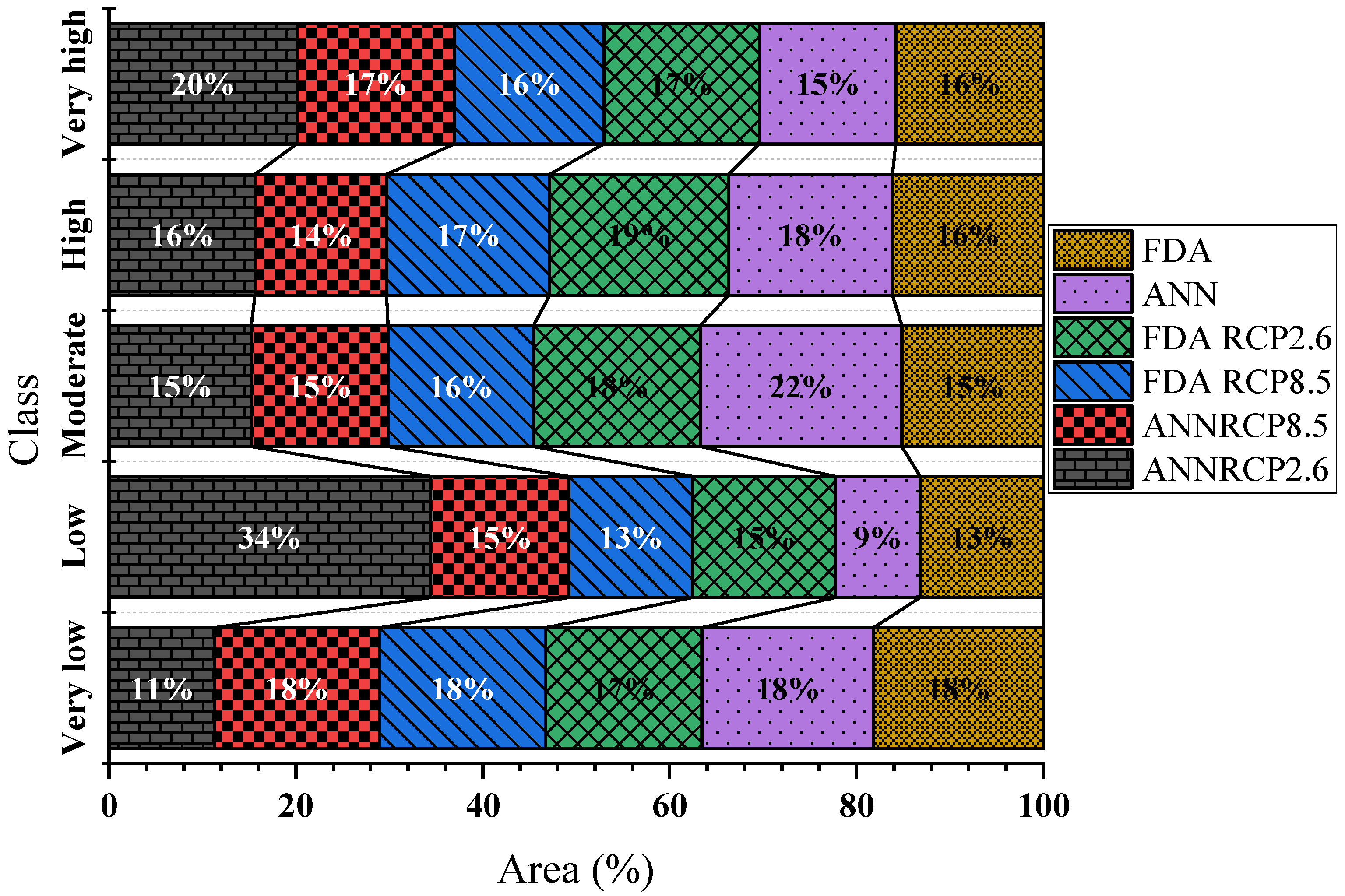
3.1. Project Climate Change
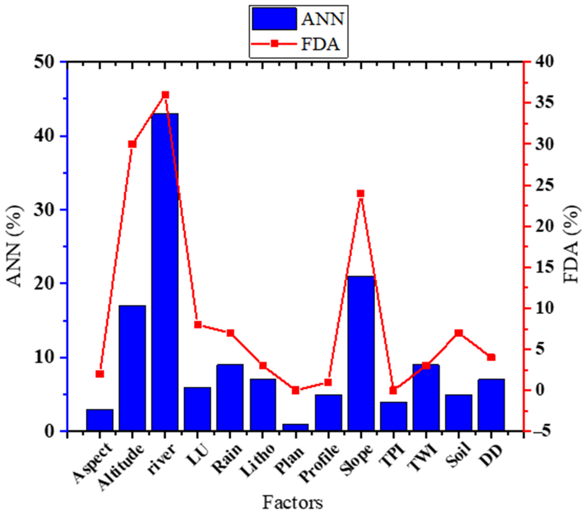
3.2. The Importance of Influencing Factors
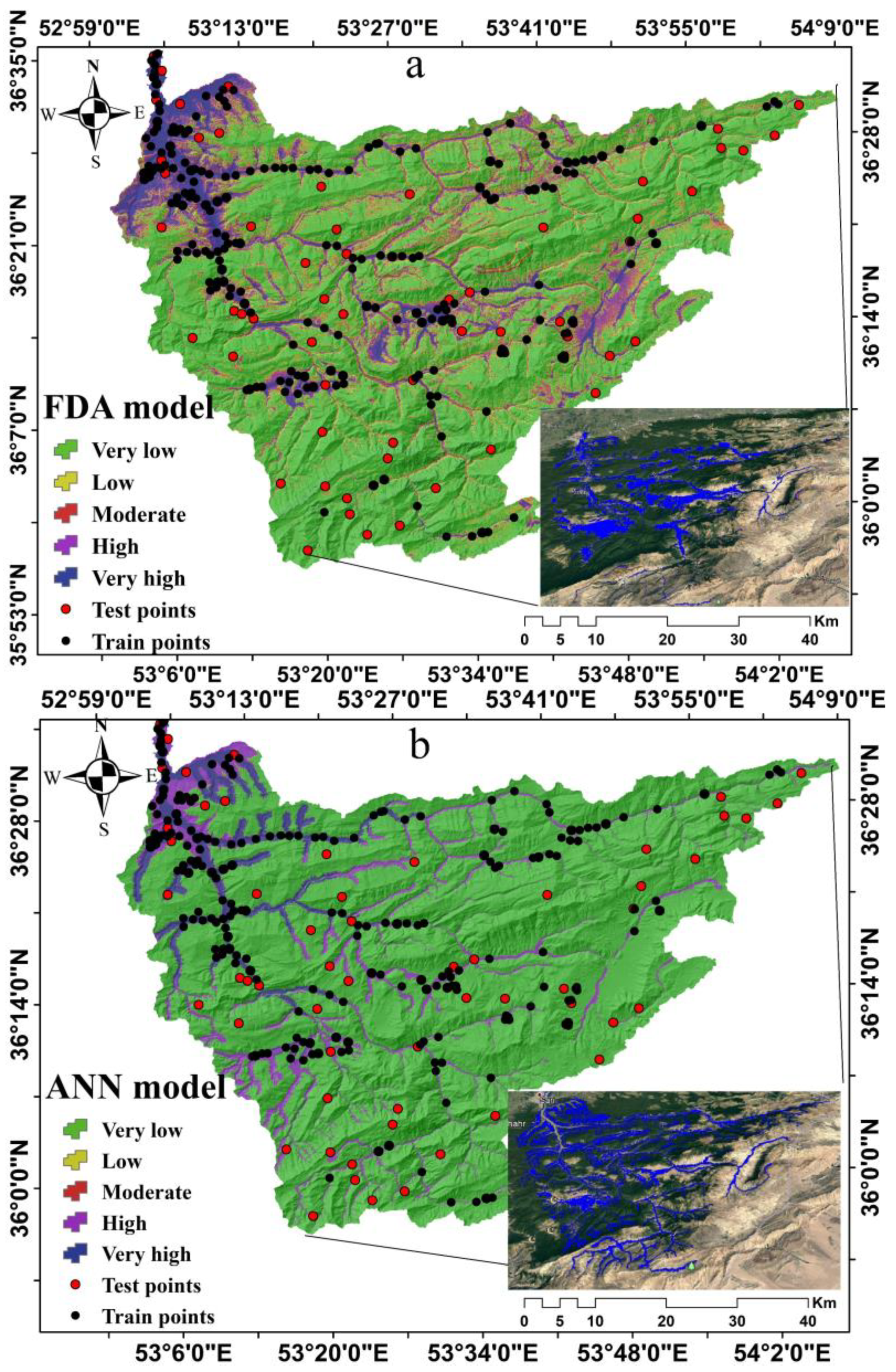
3.3. Validation Models and Maps
4. Discussion
5. Conclusions and Future Perspectives
Author Contributions
Funding
Institutional Review Board Statement
Informed Consent Statement
Conflicts of Interest
Abbreviations
| ROC | receiver operating characteristic curve |
| AUC | area under curve |
| ANN | artificial neural network |
| FDA | flexible discrimination analysis |
| TPI | terrain position index |
| TWI | topographic wetness index |
| CI | confidence interval |
| SE | standard error |
| DEM | digital elevation model |
| TSS | true skill statistic |
| POD | probability of detection |
| SR | success ratio |
References
- IPCC. Climate Change 2013. In The Physical Science Basis Working Group I Contribution to the Fifth Assessment Report of the Intergovernmental Panel on Climate Change Edited by 2013; IPCC: Geneva, Switzerland, 2013. [Google Scholar]
- Hodgkins, G.A.; Whitfield, P.H.; Burn, D.H.; Hannaford, J.; Renard, B.; Stahl, K.; Fleig, A.K.; Madsen, H.; Mediero, L.; Murphy, C.; et al. Climate-driven variability in the occurrence of major floods across North America and Europe. J. Hydrol. 2017, 552, 704–717. [Google Scholar] [CrossRef]
- Ghasemain, B.; Asl, D.T.; Pham, B.T.; Avand, M.; Nguyen, H.D.; Janizadeh, S. Shallow landslide susceptibility mapping: A comparison between classification and regression tree and reduced error pruning tree algorithms. Vietnam J. Earth Sci. 2020. [Google Scholar] [CrossRef]
- Mitsova, D. Coupling Land Use Change Modeling with Climate Projections Catchment Near Cincinnati, Ohio. ISPRS Int. J. Geo-Inf. 2014, 3, 1256–1277. [Google Scholar] [CrossRef]
- IPCC. Climate Change 2017: The Physical Science Basis; IPCC: Geneva, Switzerland, 2017. [Google Scholar]
- Liuzzo, L.; Bono, E.; Sammartano, V.; Freni, G. Analysis of spatial and temporal rainfall trends in Sicily during the 1921–2012 period. Appl. Clim. 2016, 126, 113–129. [Google Scholar] [CrossRef]
- Warming, G. Perceived community-based flood adaptation strategies under climate change in Nepal. Int. J. Glob. Warm. 2014, 6, 113–124. [Google Scholar]
- Kordrostami, S.; Tao, Z.; Karim, F.; Rahman, A. Regional Flood Frequency Analysis Using an Artificial Neural Network Model. Geoscience 2020, 10, 127. [Google Scholar] [CrossRef]
- Akter, T.; Quevauviller, P.; Eisenreich, S.J.; Vaes, G. Impacts of climate and land use changes on flood risk manage-ment for the Schijn River, Belgium. Environ. Sci. Policy 2018, 89, 163–175. [Google Scholar] [CrossRef]
- Saber, M.; Abdrabo, K.I.; Habiba, O.M.; Kantosh, S.A.; Sumi, T. Impacts of Triple Factors on Flash Flood Vulnerability in Egypt: Urban Growth, Extreme Climate, and Mismanagement. Geosciences 2020, 10, 24. [Google Scholar] [CrossRef]
- Kuriqi, A.; Ali, R.; Pham, Q.B.; Gambini, J.M.; Gupta, V.; Malik, A.; Linh, N.T.; Joshi, Y.; Anh, D.T.; Dong, X. Seasonality shift and streamflow flow variability trends in central India. Acta Geophys. 2020, 68, 1461–1475. [Google Scholar] [CrossRef]
- Senent-Aparicio, J.; Jimeno-Sáez, P.; Bueno-Crespo, A.; Pérez-Sánchez, J.; Pulido-Velázquez, D. Coupling ma-chine-learning techniques with SWAT model for instantaneous peak flow prediction. Biosyst. Eng. 2019, 177, 67–77. [Google Scholar] [CrossRef]
- Thompson, J.R.; Crawley, A.; Kingston, D.G. Future river flows and flood extent in the Upper Niger and Inner Niger Delta: GCM-related uncertainty using the CMIP5 ensemble. Hydrol. Sci. J. 2017, 62, 2239–2265. [Google Scholar] [CrossRef]
- Ali, R.; Kuriqi, A.; Kisi, O. Human–Environment Natural Disasters Interconnection in China: A Review. Climate 2020, 8, 48. [Google Scholar] [CrossRef]
- Bertilsson, L.; Wiklund, K.; Moura, I.; De Moura, O.; Veról, A.P.; Miguez, M.G. Urban flood resilience—A multi-criteria index to integrate flood resilience into urban planning. J. Hydrol. 2019, 573, 970–982. [Google Scholar] [CrossRef]
- Almasi, P.; Soltani, S. Assessment of the climate change impacts on flood frequency (case study: Bazoft Basin, Iran). Stoch. Environ. Res. Risk Assess. 2016, 31, 1171–1182. [Google Scholar] [CrossRef]
- Shahabi, H.; Jarihani, B.; Piralilou, S.T.; Chittleborough, D.; Avand, M.; Ghorbanzadeh, O. A Semi-Automated Object-Based Gully Networks Detection Using Different Machine Learning Models: A case study of Bowen Catchment, Queensland, Australia. Sensor 2019, 19, 4893. [Google Scholar] [CrossRef]
- Yariyan, P.; Avand, M.; Abbaspour, R.A.; Haghighi, A.T.; Costache, R.; Ghorbanzadeh, O.; Janizadeh, S.; Blaschke, T. Flood susceptibility mapping using an improved analytic network process with statistical models. Geomat. Nat. Hazards Risk 2020, 11, 2282–2314. [Google Scholar] [CrossRef]
- Talukdar, S.; Ghose, B.; Salam, R.; Mahato, S.; Pham, Q.B.; Linh, N.T.T.; Avand, M. Flood susceptibility modeling in Teesta River basin, Bang-ladesh using novel ensembles of bagging algorithms. Stoch. Environ. Res. Risk Assess. 2020, 34, 2277–2300. [Google Scholar] [CrossRef]
- Abdelkarim, A.; Al-Alola, S.S.; Alogayell, H.M.; Mohamed, S.A.; Alkadi, I.I.; Youssef, I.Y. Mapping of GIS-Flood Hazard Using the Geomorphometric-Hazard Model: Case Study of the Al-Shamal Train Pathway in the City of Qurayyat, Kingdom of Saudi Arabia. Geosciences 2020, 10, 333. [Google Scholar] [CrossRef]
- Avand, M.; Janizadeh, S.; Tien Bui, D.; Pham, V.H.; Ngo, P.T.; Nhu, V.H. A tree-based intelligence ensemble approach for spatial prediction of potential groundwater. Int. J. Digit. Earth 2020, 1–22. [Google Scholar] [CrossRef]
- Garner, A.J.; Mann, M.E.; Emanuel, K.A.; Kopp, R.E.; Lin, N.; Alley, R.B.; Horton, B.P.; DeConto, R.M.; Donnelly, J.P.; Pollard, D. Impact of climate change on New York City’s coastal flood hazard: Increasing flood heights from the preindustrial to 2300 CE. Proc. Natl. Acad. Sci. USA 2017, 114, 11861–11866. [Google Scholar] [CrossRef]
- Hirabayashi, Y.; Mahendran, R.; Koirala, S.; Konoshima, L.; Yamazaki, D.; Watanabe, S.; Kim, H.; Kanae, S. Global flood risk under climate change. Nat. Clim. Chang. 2013, 3, 816–821. [Google Scholar] [CrossRef]
- Dobler, C.; Bürger, G.; Stötter, J. Assessment of climate change impacts on flood hazard potential in the Al-pine Lech watershed. J. Hydrol. 2012, 460, 29–39. [Google Scholar] [CrossRef]
- Dankers, R.; Feyen, L. Flood hazard in Europe in an ensemble of regional climate scenarios. J. Geophys. Res. Atmos. 2009, 114, 114. [Google Scholar] [CrossRef]
- Islam, A.R.M.T.; Talukdar, S.; Mahato, S.; Kundu, S.; Eibek, K.U.; Pham, Q.B.; Kuriqi, A.; Linh, N.T. Flood susceptibility modelling using advanced ensemble machine learning models. Geosci. Front. 2020. [Google Scholar] [CrossRef]
- Mendizabal, M.; Sepúlveda, J.; Torp, P. Climate change impacts on flood events and its consequences on hu-man in Deba River. Int. J. Environ. Res. 2014, 8, 221–230. [Google Scholar]
- Roy, P.; Pal, S.C.; Chakrabortty, R.; Chowdhuri, I.; Malik, S.; Das, B. Threats of climate and land use change on future flood susceptibility. J. Clean. Prod. 2020, 272, 122757. [Google Scholar] [CrossRef]
- Xie, H.; Hu, X.J. Time-Series Data Mining of Minimum Design Height for River Bridge Deck Using Seasonal Trend Decomposition. Phys. Conf. Ser. 2019, 1284, 012042. [Google Scholar] [CrossRef]
- Jung, C.; Lee, J.-W.; Lee, Y.; Kim, S.-J. Quantification of Stream Drying Phenomena Using Grid-Based Hydrological Modeling via Long-Term Data Mining throughout South Korea including Ungauged Areas. Water 2019, 11, 477. [Google Scholar] [CrossRef]
- Salih, S.Q.; Sharafati, A.; Khosravi, K.; Faris, H. River suspended sediment load prediction based on riv-er discharge information: Application of newly developed data mining models. Hydrol. Sci. J. 2020, 65, 624–637. [Google Scholar] [CrossRef]
- Moradi, H.R.; Avand, M.T.; Janizadeh, S. Spatial Modeling in GIS and R for Earth and Environmental Sciences; Elsevier: Amsterdam, The Netherlands, 2019; pp. 259–275. [Google Scholar]
- Hassani, H.; Huang, X.; Silva, E.S. Big Data and Climate Change. Big Data Cogn. Comput. 2019, 3, 12. [Google Scholar] [CrossRef]
- Khosravi, K.; Daggupati, P.; Alami, M.T.; Awadh, S.M.; Ghareb, M.I.; Panahi, M.; Pham, B.T.; Rezaie, F.; Qi, C.; Yaseen, Z.M. Meteorological data mining and hybrid data-intelligence models for reference evaporation simulation: A case study in Iraq. Comput. Electron. Agric. 2019, 167, 105041. [Google Scholar] [CrossRef]
- Rajaei, F.; Esmaili, A.; Abdolrassoul, S. Surface drainage nitrate loading estimate from agriculture fields and its relationship with landscape metrics in Tajan watershed. Paddy Water Environ. 2017, 15, 541–552. [Google Scholar] [CrossRef]
- Bui, D.T.; Tsangaratos, P.; Ngo, P.T.T.; Pham, T.D.; Pham, B.T. Flash flood susceptibility modeling using an optimized fuzzy rule based feature selection technique and tree based ensemble methods. Sci. Total Environ. 2019, 668, 1038–1054. [Google Scholar] [CrossRef] [PubMed]
- Pham, B.T.; Avand, M.; Janizadeh, S.; Van Phong, T.; Al-Ansari, N.; Ho, L.S.; Das, S.; Van Le, H.; Amini, A.; Bozchaloei, S.K.; et al. GIS Based Hybrid Computational Approaches for Flash Flood Susceptibility Assessment. Water 2020, 12, 683. [Google Scholar] [CrossRef]
- Costache, R.; Pham, Q.B.; Sharifi, E.; Linh, N.T.T.; Abba, S.I.; Vojtek, M.; Vojteková, J.; Nhi, P.T.T.; Khoi, D.N. Flash-Flood Susceptibility Assessment Using Multi-Criteria Decision Making and Machine Learning Supported by Remote Sensing and GIS Techniques. Remote Sens. 2019, 12, 106. [Google Scholar] [CrossRef]
- Tehrany, M.S.; Pradhan, B.; Jebur, M.N. Flood susceptibility mapping using a novel ensemble weights-of-evidence and support vector machine models in GIS. J. Hydrol. 2014, 512, 332–343. [Google Scholar] [CrossRef]
- Chapi, K.; Singh, V.P.; Shirzadi, A.; Shahabi, H.; Bui, D.T.; Pham, B.T.; Khosravi, K. A novel hybrid artificial intelligence approach for flood susceptibility assessment. Environ. Model. Softw. 2017, 95, 229–245. [Google Scholar] [CrossRef]
- Al-Juaidi, A.E.M.; Nassar, A.M.; Al-Juaidi, O.E.M. Evaluation of flood susceptibility mapping using logistic regression and GIS conditioning factors. Arab. J. Geosci. 2018, 11, 765. [Google Scholar] [CrossRef]
- Lee, M.-J.; Kang, J.-E.; Jeon, S. Application of frequency ratio model and validation for predictive flooded area susceptibility mapping using GIS. In Proceedings of the 2012 IEEE International Geoscience and Remote Sensing Symposium, Munich, Germany, 22–27 July 2012. [Google Scholar]
- Zhao, G.; Pang, B.; Xu, Z.; Peng, D.; Xu, L. Assessment of urban flood susceptibility using semi-supervised machine learning model. Sci. Total Environ. 2019, 659, 940–949. [Google Scholar] [CrossRef]
- Pradhan, B. Journal of Spatial Hydrology Biswajeet Pradhan. J. Spat. Hydrol. 2009, 9, 1–18. [Google Scholar]
- Pradhan, B.; Youssef, A.M. A100-year maximum flood susceptibility mapping using integrated hydrological and hydrodynamic models: Kelantan River Corridor, Malaysia. J. Flood Risk Manag. 2011, 4, 189–202. [Google Scholar] [CrossRef]
- Nachappa, T.G.; Piralilou, S.T.; Gholamnia, K.; Ghorbanzadeh, O.; Rahmati, O.; Blaschke, T. Flood susceptibility mapping with machine learning, multi-criteria decision analysis and ensemble using Dempster Shafer Theory. J. Hydrol. 2020, 590, 125275. [Google Scholar] [CrossRef]
- Costache, R.; Popa, M.C.; Bui, D.T.; Diaconu, D.C.; Ciubotaru, N.; Minea, G.; Pham, Q.B. Spatial predicting of flood potential areas using novel hybridizations of fuzzy decision-making, bivariate statistics, and machine learning. J. Hydrol. 2020, 585, 124808. [Google Scholar] [CrossRef]
- Rahmati, O.; Pourghasemi, H.R.; Zeinivand, H. Flood susceptibility mapping using frequency ratio and weights-of-evidence models in the Golastan Province, Iran. Geocarto Int. 2016, 31, 42–70. [Google Scholar] [CrossRef]
- Costache, R. Flood Susceptibility Assessment by Using Bivariate Statistics and Machine Learning Models-A Useful Tool for Flood Risk Management. Water Resour. Manag. 2019, 1–18. [Google Scholar] [CrossRef]
- Costache, R.; Pham, Q.B.; Avand, M.; Linh, N.T.T.; Vojtek, M.; Vojteková, J.; Dung, T.D. Novel hybrid models between bivariate statistics, ar-tificial neural networks and boosting algorithms for flood susceptibility assessment. J. Environ. Manag. 2020, 265, 110485. [Google Scholar] [CrossRef]
- Hastie, T.; Tibshirani, R.; Friedman, J. The Elements of Statistical Learning: Data Mining, Inference, and Prediction; Springer: Berlin/Heidelberg, Germany, 2009. [Google Scholar]
- Ashrafzadeh, M.R.; Naghipour, A.A.; Haidarian, M.; Khorozyan, I. Modeling the response of an endangered flagship predator to climate change in Iran. Mammal Res. 2018, 64, 39–51. [Google Scholar] [CrossRef]
- Hastie, T.; Tibshirani, R.; Buja, A. Flexible Discriminant and Mixture Models; Stanford University: Stanford, CA, USA, 1995. [Google Scholar]
- Roth, V.; Steinhage, V. Nonlinear discriminant analysis using kernel functions. Adv. Neural Inf. Process. Syst. 1999, 12, 568–574. [Google Scholar]
- Dawson, C.W.; Abrahart, R.J.; Shamseldin, A.Y.; Wilby, R.L. Flood estimation at ungauged sites using artifi-cial neural networks. J. Hydrol. 2006, 319, 391–409. [Google Scholar] [CrossRef]
- Pradhan, B.; Lee, S.; Buchroithner, M.F. A GIS-based back-propagation neural network model and its cross-application and validation for landslide susceptibility analyses. Comput. Environ. Urban Syst. 2010, 34, 216–235. [Google Scholar] [CrossRef]
- Mukerji, A.; Chatterjee, C.; Raghuwanshi, N.S. Flood Forecasting Using ANN, Neuro-Fuzzy, and Neuro-GA Models. J. Hydrol. Eng. 2009, 14, 647–652. [Google Scholar] [CrossRef]
- Pham, B.T.; Jaafari, A.; Avand, M.; Al-Ansari, N.; Du, T.D.; Yen, H.P.H.; Van Phong, T.; Nguyen, H.D.; Van Le, H.; Mafi-Gholami, D.; et al. Performance Evaluation of Machine Learning Methods for Forest Fire Modeling and Prediction. Symmetry 2020, 12, 1022. [Google Scholar] [CrossRef]
- Lei, X.; Chen, W.; Avand, M.; Janizadeh, S.; Kariminejad, N.; Shahabi, H.; Costache, R.; Shahabi, H.; Shirzadi, A.; Mosavi, A. GIS-Based Machine Learning Algorithms for Gully Erosion Susceptibility Mapping in a Semi-Arid Region of Iran. Remote Sens. 2020, 12, 2478. [Google Scholar] [CrossRef]
- Pham, B.T.; Van Phong, T.; Avand, M.; Al-Ansari, N.; Singh, S.K.; Van Le, H.; Prakash, I. Improving Voting Feature Intervals for Spatial Prediction of Landslides. Math. Probl. Eng. 2020, 2020, 4310791. [Google Scholar] [CrossRef]
- Yousefi, S.; Avand, M.; Yariyan, P.; Pourghasemi, H.R.; Keesstra, S.; Tavangar, S.; Tabibian, S. A novel GIS-based ensemble technique for rangeland downward trend mapping as an ecological indicator change. Ecol. Indic. 2020, 117, 106591. [Google Scholar] [CrossRef]
- Avand, M.; Moradi, H.; Ramazanzadeh, M. Using machine learning models, remote sensing, and GIS to investigate the effects of changing climates and land uses on flood probability. J. Hydrol. 2020, 125663. [Google Scholar] [CrossRef]
- Avand, M.; Janizadeh, S.; Naghibi, S.A.; Pourghasemi, H.R. A Comparative Assessment of Random Forest and k-Nearest Neighbor Classifiers for Gully Erosion Susceptibility Mapping. Water 2019, 11, 2076. [Google Scholar] [CrossRef]
- Costache, R.; Țincu, R.; Elkhrachy, I.; Pham, Q.B.; Popa, M.C.; Diaconu, D.C.; Bui, D.T. New neural fuzzy-based machine learning ensem-ble for enhancing the prediction accuracy of flood susceptibility mapping. Hydrol. Sci. J. 2020, 65, 2816–2837. [Google Scholar] [CrossRef]
- Ahmadlou, M.; Karimi, M.; Alizadeh, S.; Shirzadi, A.; Parvinnejhad, D.; Shahabi, H.; Panahi, M. Flood susceptibility assessment using integration of adaptive network-based fuzzy inference system (ANFIS) and biogeography-based optimization (BBO) and BAT algo-rithms (BA). Geocarto Int. 2019, 34, 1252–1272. [Google Scholar] [CrossRef]
- Shafizadeh-Moghadam, H.; Valavi, R.; Shahabi, H.; Chapi, K.; Shirzadi, A. Novel forecasting approaches us-ing combination of machine learning and statistical models for flood susceptibility mapping. J. Environ. Manag. 2018, 217, 1–11. [Google Scholar] [CrossRef]
- Nourani, V.; Mousavi, S. Spatiotemporal groundwater level modeling using hybrid artificial intelligence-meshless method. J. Hydrol. 2016, 536, 10–25. [Google Scholar] [CrossRef]
- Tehrany, M.S.; Pradhan, B.; Jebur, M.N. Flood susceptibility analysis and its verification using a novel ensem-ble support vector machine and frequency ratio method. Stoch. Environ. Res. Risk Assess. 2015, 29, 1149–1165. [Google Scholar] [CrossRef]


| Number | Code | Description | Age |
|---|---|---|---|
| 1 | Cm | Dark grey to black fossiliferous limestone with subordinate black shale (MOBARAK FM) | Carboniferous |
| 2 | Dbsh | Undifferentiated limestone, shale, and marl | Devonian |
| 3 | Dj | Yellowish, thin to thick-bedded, fossiliferous argillaceous limestone, dark grey limestone, greenish marl, and shale, locally including gypsum | Devonian |
| 4 | E | Nummulitic limestone | Eocene |
| 5 | E1 | Dark red medium-grained arkosic to subarkosic sandstone and micaceous siltstone (LALUN FM) | Cambrian |
| 6 | E2l2 | Globotrunca limestone | Late.Cretaceous |
| 7 | Ebt | Alternation of dolomite, limestone, and variegated shale (BARUT FM) | Cambrian |
| 8 | Em | Dolomite platy and flaggy limestone containing trilobite; sandstone and shale (MILA FM) | Cambrian |
| 9 | Ez | Reef-type limestone and gypsiferous marl (ZIARAT FM) | Paleocene-Eocene |
| 10 | J | Light grey, thin-bedded to massive limestone (LAR FM) | Jurassic-Cretaceous |
| 11 | K1l | Thick bedded to massive, white to pinkish orbitolina bearing limestone (TIZKUH FM) | Early.Cretaceous |
| 12 | K2 | Hyporite bearing limestone (Senonian) | Late.Cretaceous |
| 13 | K2plm | Thick-bedded to massive limestone (maastrichtian) | Late.Cretaceous |
| 14 | Mc | Red conglomerate and sandstone | Miocene |
| 15 | Msm | Marl, calcareous sandstone, sandy limestone, and minor conglomerate | Miocene |
| 16 | Pd | Red sandstone and shale with subordinate sandy limestone (DORUD FM) | Permian |
| 17 | Pec | Light-red coarse-grained, a polygenic conglomerate with sandstone intercalations | Paleocene-Eocene |
| 18 | PEk | Dull green grey slaty shales with subordinate intercalation of quartzitic sandstone (KAHAR FM; Morad series and Kalmard Fm) | Pre-Cambrian |
| 19 | Pel | Medium to thick-bedded limestone | Paleocene-Eocene |
| 20 | PEm | Marl and gypsiferous marl locally gypsiferous mudstone | Paleocene-Eocene |
| 21 | Plc | Polymictic conglomerate and sandstone | Pliocene |
| 22 | Pr | Dark grey medium-bedded to massive limestone (RUTEH LIMESTONE) | Permian |
| 23 | Qt | High-level piedmont fan and valley terrace deposits | Quaternary |
| 24 | TRe | Thin bedded, yellow to pinkish argillaceous limestone with worm tracks | Triassic |
| 25 | URig | Red marl, gypsiferous marl, sandstone, and conglomerate (Upper red Fm.) | Miocene |
| Criteria | AUC | SE | %CI | Accuracy | TSS | Kappa | Bias | SR | POD | |
|---|---|---|---|---|---|---|---|---|---|---|
| Model | ||||||||||
| FDA | 0.918 | 0.038 | 0.799 to 0.936 | 0.86 | 0.78 | 0.72 | 0.82 | 0.89 | 0.92 | |
| ANN | 0.897 | 0.042 | 0.761 to 0.90 | 0.82 | 0.69 | 0.71 | 0.86 | 0.84 | 0.90 | |
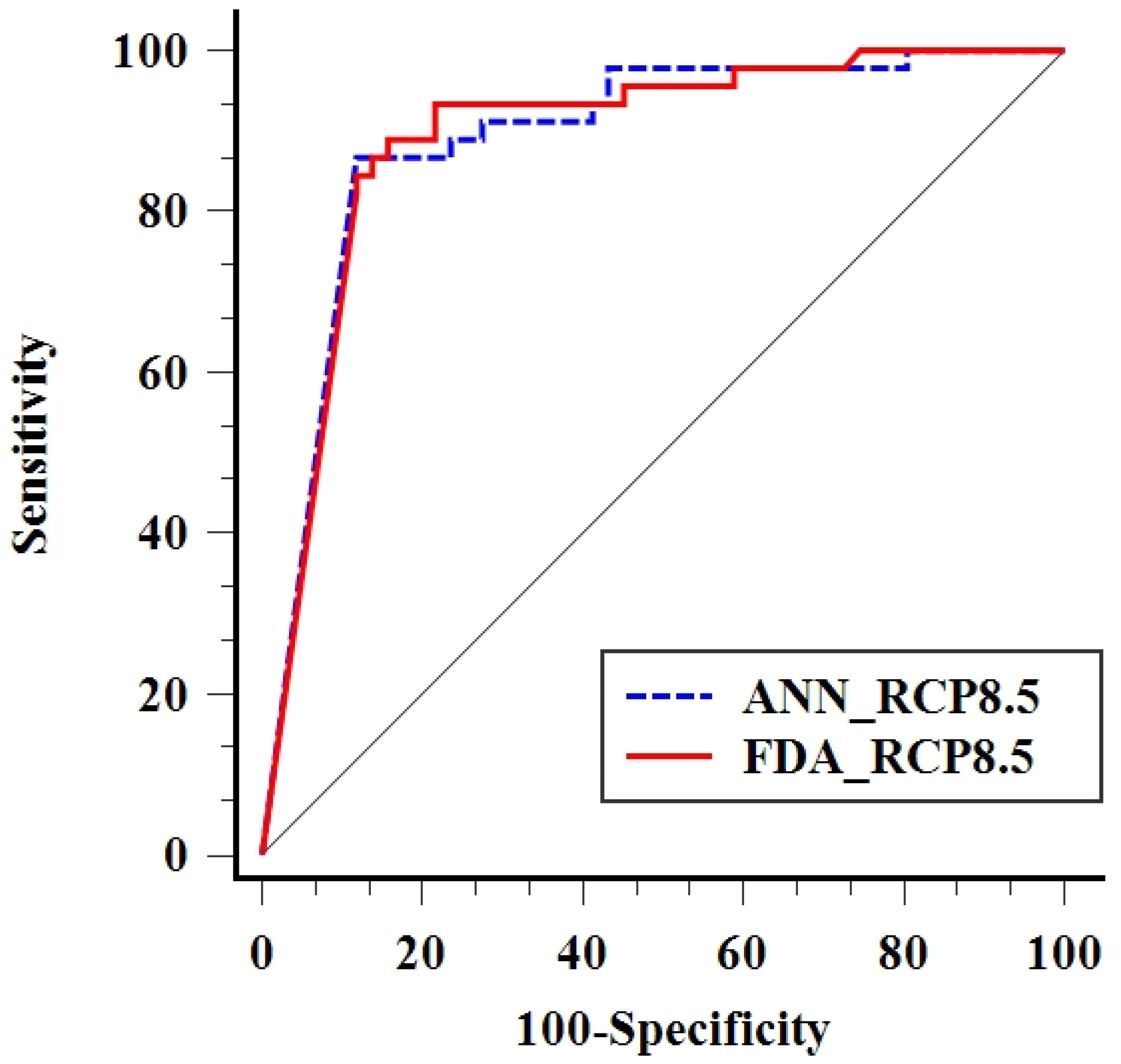
| Criteria | AUC | SE | 95% CI | |
|---|---|---|---|---|
| Models | ||||
| ANN RCP2.6 | 0.888 | 0.035 | 0.80 to 0.94 | |
| ANN RCP8.5 | 0.892 | 0.032 | 0.81 to 0.94 | |
| FDA RCP2.6 | 0.910 | 0.032 | 0.83 to 0.95 | |
| FDA RCP8.5 | 0.893 | 0.032 | 0.81 to 0.94 | |
Publisher’s Note: MDPI stays neutral with regard to jurisdictional claims in published maps and institutional affiliations. |
© 2021 by the authors. Licensee MDPI, Basel, Switzerland. This article is an open access article distributed under the terms and conditions of the Creative Commons Attribution (CC BY) license (http://creativecommons.org/licenses/by/4.0/).
Share and Cite
Avand, M.; Moradi, H.R.; Ramazanzadeh Lasboyee, M. Spatial Prediction of Future Flood Risk: An Approach to the Effects of Climate Change. Geosciences 2021, 11, 25. https://doi.org/10.3390/geosciences11010025
Avand M, Moradi HR, Ramazanzadeh Lasboyee M. Spatial Prediction of Future Flood Risk: An Approach to the Effects of Climate Change. Geosciences. 2021; 11(1):25. https://doi.org/10.3390/geosciences11010025
Chicago/Turabian StyleAvand, Mohammadtaghi, Hamid Reza Moradi, and Mehdi Ramazanzadeh Lasboyee. 2021. "Spatial Prediction of Future Flood Risk: An Approach to the Effects of Climate Change" Geosciences 11, no. 1: 25. https://doi.org/10.3390/geosciences11010025
APA StyleAvand, M., Moradi, H. R., & Ramazanzadeh Lasboyee, M. (2021). Spatial Prediction of Future Flood Risk: An Approach to the Effects of Climate Change. Geosciences, 11(1), 25. https://doi.org/10.3390/geosciences11010025