Heated Topics in Thermochronology and Paths towards Resolution

Abstract

Thermochronometry is widely used to track exhumation, the motion of rock towards Earth’s surface, and to gain fresh insights into geodynamic and geomorphic processes. Applications require models to reconstruct a rock’s cooling history as it is exhumed from higher temperatures at depth within the crust to cooler shallower levels and eventually Earth’s surface. Thermochronometric models are dependent on the predictable accumulation and the temperature-dependent loss of radiogenic daughter products measured in the laboratory. However, there are many geologically reasonable scenarios that will yield very similar thermochronometric ages. This similarity hinders finding the actual scenario, so instead an approximate model is sought. Finding suitable model parameters is a potentially ill-posed inverse problem that requires making decisions about how best to extract information from the data and how to combine data to leverage redundant information and reduce the impact of data noise. Often these decisions lead to differences in conclusions of studies and such discrepancies have led to heated debates. Here, we discuss debates centred on the use of a variety of modelling approaches and potential sources of biases that lead to differences in the predicted exhumation rate. We also provide some suggestions about future research paths that will help resolve these debates.

1. Introduction

Inverse problems can be unintuitive. Whereas a forward model, or simulation, has a single solution for a combination of model parameters, there may be many other combinations of model parameters that also provide the same, or a very similar, solution, even for perfect, noise-free data. These sorts of inverse problems are used extensively across the Earth Sciences from large-scale seismic tomographic inversions with thousands of model parameters describing the velocity structure of the Earth [1] to two-parameter linear regressions through geomorphic datasets with just a slope and intercept [2]. However, challenges associated with the design, implementation, interpretation and appraisal of these types of inverse models have resulted in long-standing debates within the thermochronology community regarding various geologic problems. In particular, it is unclear whether mountain belt erosion rates increased over the course of the Neogene or whether this is an artefact of different inverse modelling methodologies [3,4,5,6,7]. This fundamental geological problem, of whether an increase in mountain rock uplift and erosion rates triggered northern hemisphere glaciation through weathering feedback mechanisms or glaciation and climate change triggered an increase in erosion which has been mistaken for an increase in rock uplift, remains debated. Here, we distil some of these debates and attempt to explain the underlying challenges faced by researchers who utilise thermochronological data. Our goal is to simplify these discussions and highlight solutions and practical ways forward.

Thermochronology methods provide estimates of thermal histories over a range of time intervals (from thousands of years to hundreds of millions of years), and are therefore useful for constraining the rates of exhumation (i.e., the motion of rocks relative to Earth’s surface) and burial. The predictable decay rates of radioactive nuclides, along with measurements of the relative abundances of those nuclides and the resulting daughter products, provide the basis of radiogenic nuclide geochronology. The difference between geochronometers and thermochronometers is that for thermochronometric systems, the daughter products are only retained at low temperatures, when diffusive loss through geologic time is negligible [8]. At high temperatures, the daughter product is lost at the same rate it is produced; thus, no daughter products accumulate. However, at sufficiently low temperatures, all of the daughter products are retained in the crystal (i.e., “closed system” behaviour) and accumulation of daughter products continues at the rate of production. In turn, the apparent age can be interpreted as corresponding to cooling below a specific ‘closure’ temperature, [9]. Since temperature increases with depth, and if the depth to the ‘closure’ temperature can be estimated, a thermochronometric age can be converted to an exhumation rate. In general, therefore, a single age (+uncertainty) provides a single exhumation rate (+uncertainty).

Many interesting tectonic and geomorphic problems are related to identifying past changes in exhumation rates as a function of space and time: When was this fault active? When did this glacial valley form? Did past changes in climate drive changes in erosion rates or was this the other way round? How and when do deep mantle processes dynamically cause Earth’s surface to uplift? Such questions require more information than is contained in a single age to identify and quantify past changes in cooling and exhumation rates. Some thermochronometric systems contain additional information that can constrain features of a thermal history and these are discussed below. Alternatively, information contained in different ages can be combined. Multiple ages from the same rock sample can be obtained using different thermochronometric with different closure temperatures. Alternatively, multiple samples that are near each other can be analysed at the same time with a model, exploiting the concept that samples have experienced similar but slightly different exhumation histories.

Here, we highlight the importance and limitations of different inverse methods designed to extract information from thermochronometric data. We begin by describing methods that have been used to extract time-temperature information from thermochronometric data with a focus on time-temperature path inversions. These approaches rest close to the data in that the data are primarily sensitive to the temperature history but have limited input in terms of physical or geological parameters (such as geothermal gradients, heat flow, thermal conductivities, heat transfer processes). In many cases geological interpretations require conversion of thermochronometric ages or time-temperature paths to exhumation rates, and therefore we examine some of the approaches used. These approaches rest further from the data in that they assume physical parameters, or models, to force samples to share similar thermal histories, thereby utilising redundant information. Therefore, we discuss some of the associated complications that can be transformed into opportunities. We review questions that have been raised about the success of these inverse methods and whether they can resolve recent changes in exhumation or are strongly affected by biases.

2. Thermal History Modelling of Thermochronometric Data

To obtain the thermal history of a sample of rock is a fundamental goal in thermochronometry. Predicted thermal histories from inverse models are then compared to different geological scenarios. The thermal history information that can be extracted from a single age is limited: there are many time-temperature paths that will give the same thermochronometric age. Consequently, any subsequent inference of exhumation rates will be similarly non-unique. The degree of non-uniqueness comes from two different sources. The first source is that samples may spend a considerable amount of time at a temperature that is approximately the closure temperature. In this scenario, a thermochronometric age does not record closure at all. Instead it represents a balance between the production of radiometric daughter products and their diffusive loss. The second source of non-uniqueness is related to processes that occur once the rock has cooled well below the closure temperature. During this time interval, the sample may cool rapidly to the surface, undergo minor reburial (but remain below the closure temperature), then cool again, or it might cool gradually to surface temperatures. However, because a given system may not be sensitive to lower temperatures, the age is insensitive to these aspects of the thermal history. One solution to this problem is to use multiple thermochronometric systems. A preliminary thermal history can be inferred by plotting thermochronometric ages against their nominal closure temperatures. The slope of this line gives an apparent cooling rate over the time intervals constrained by the data. This approach, however, fails to account for the cooling rate dependence on closure temperature and there are other thermochronometric aspects that can be exploited to reveal complex thermal histories.

Radiogenic ⁴⁰Ar (i.e., produced by the decay of ⁴⁰K) begins to be retained in micas at relatively high temperatures (~400–300 °C). In this system, it is thought that there is a range of crystallographic shapes, sizes and compositions that effectively have different temperature sensitivity and sample analyses exploit this by controlled extraction of ⁴⁰Ar from these different ‘diffusion domains’ as a function of temperature. By inferring the relative distribution of these domains it is possible to recover a continuous cooling history since the domains have overlapping temperature sensitivity [10]. As argon data generally record metamorphic temperatures and cooling through the ductile-brittle transition zone, most geological studies use lower temperature chronometers to extract upper-crustal thermal histories.

Fission track analysis is perhaps the most commonly used thermochronometer, since not only can the closure temperature concept be applied, but also additional constraints on the cooling path can be obtained from the track length distribution. All tracks are produced with approximately the same length, approximately 16–17 µm in apatite, but heating will anneal, or shorten, a track length until, at ~110–120 °C, over geological time, tracks in apatite are completely annealed [11,12]. Since tracks are produced continuously throughout geological time, each preserved track in a sample will have been exposed to a different portion of the time and temperature history of its host rock. The distribution of lengths thus provides an integrated record of that sample’s thermal history below temperatures of ~110–120 °C to approximately 60 °C, at which point levels of annealing are minor. The age data provide information on the overall duration, and sometimes specific events, of the thermal history.

At even lower temperatures (~80–30 °C), radiogenic ⁴He (i.e., produced along the U and Th decay series) is retained in apatite crystals. The diffusion kinetics are controlled by numerous factors but grain size, composition, radiation damage (damage to the crystal lattice produced by nuclear decay events), and whether or not the complete crystal was analysed appear to be the most important. Therefore apatite (U-Th)/He ages from the same sample, may be very different, or dispersed. If these factors can be appropriately accounted for, these different ages can be exploited to infer a thermal history [13,14]. In this respect, the (U-Th)/He system in apatite provides several thermochronometers in one. Furthermore, if the spatial distribution of ⁴He within an individual apatite crystal can be observed or inferred, it further constrains the continuous thermal paths that produced this distribution by the competing processes of helium production and diffusive loss [15].

These different methods can be used to reconstruct models of thermal histories, but the challenge is in how to judge which models/outputs are realistic, and how to incorporate other types of data. These lead to decisions that have had to be made at different stages in the interpretation process from the design of some of the widely used algorithms to implementation of modelling tools.

3. Extracting Thermal History Information from Thermochronometric Data

The two most commonly used software tools designed to extract information from single samples with AFT and AHe data are HeFTy [16] and QTQt [17]. These two approaches are based on different concepts but usually result in similar output thermal histories. However, an article by Vermeesch and Tian (2014) [18] highlighted how, without careful use, these different underlying concepts could cause the algorithms to break or lead to mistakes in interpreting the results. This topic, which has seen ongoing debate, [19,20,21,22,23] reflects many of the complexities inherent to inverse problems. Below, we attempt to simplify this debate. Both of these approaches parameterise a thermal history in terms of a series of time-temperature points that are connected by linear interpolation to form the model thermal history. Neither incorporate any heat transfer processes (diffusion, advection), but also avoid the need to specify additional thermophysical parameters.

HeFTy generates random time-temperature paths that are often forced to pass through user defined boxes and the resultant model predictions are compared with observations. If the agreement is acceptable or good based on a p-value-based hypothesis test, the paths are kept and plotted in pink and green (good and acceptable fits), respectively. However, if a model cannot be found that passes the specified test, no paths are shown. The p-value test is most likely to fail for noisy data, data that have very small measurement uncertainties, or, for when the implicit assumption behind the model that all crystals analysed share a common thermal history breaks down [24]. The risk of not selecting many paths is exacerbated by the fact that HeFTy uses a purely random path generation algorithm, reducing the overall search efficiency. Whilst this random-search procedure means that the algorithm does not learn which aspects of a thermal history are promising and thus can waste time searching parameter space to which the data are not sensitive, random searches also have advantages. If there is an alternative set of time-temperature paths that are favourable, a random algorithm will find these (with sufficient model runs), but an approach that learns from previous sampling may get stuck with sets of parameters that represent a local minimum of misfit space. QTQt instead uses a reversible jump Markov Chain Monte Carlo (rj-MCMC) algorithm to sample the posterior, and generate paths based on posterior probability. The results of the algorithm can be viewed as a probability plot showing the rock’s temperature at any time conditional on other parts of parameter space. However, it is important to note that a new path that traverses the highest probability peaks may not do a good job at explaining the data. In addition, there is no guarantee that the best models will fit the data very well. This is because the MCMC algorithm simply compares relative posterior probabilities to find the better models. The lack of a guarantee that the best models are good means that it might be tricky to identify when fundamental assumptions are broken or when the data are problematic. However, it is easy to check the data fit by inspecting the predictions afterwards. In addition, the reversible jump component of the algorithm provides a means to determine how complex the time-temperature path should be based on the data and any other constraints although this can lead to models that are overly simple.

Figure 1 highlights the sorts of results that are expected if a single age is inverted with HeFTy or QTQt. We do not recommend that a single age should be interpreted in this way—this is just for illustrative purposes. The true path is shown in the black line. HeFTy will produce a range of time-temperature paths that have variable levels of complexity, where the complexity in this example would be controlled by user-defined constraints on the rates of temperature change or the number of inflection points. This is known as model damping and represents additional information that is incorporated into the model. QTQt would produce similar paths, but more paths would be generated that have a constant cooling rate, as this is the simplest model that explains the data. This results in a posterior probability that favours these simple models, to the point at which the true model is outside the area of maximum probability. Clearly, a single age giving a single cooling rate (+uncertainty) is the most sensible solution, but there may be cases where the simplest model is not correct. Of course, if the thermal history is consistent with the data, we need additional information to decide that it is not correct and there will always be aspects of the geological record that are uncertain. This concept is also true for more complicated cooling histories as shown by [20]. If no model damping is introduced, then thermal histories that oscillate wildly are just as good, in that they fit the data just as well, as less variable thermal histories. In other words, lots of models do an equally good job at explaining data [23]. Clearly, we want to make a choice of preferred model or models, and something else is required to extract representative thermal history information from the data.

3.1. Correlations amongst Aspects of a Thermal History

It is also worth considering how model parameters may be correlated, as this may determine some of the most important aspects of a particular thermal history. For example, the total amount of fission track shortening is a function of both temperature and time. If a rock is heated to a specific temperature for a specific amount of time, the same amount of shortening may be expected for a slightly higher temperature for a shorter amount of time. If the data are mainly sensitive to burial conditions, rapid cooling to surface temperatures may be driven by the requirement for long durations of burial as opposed to recent cooling. In other words, the burial conditions may be closely linked to subsequent cooling and any geological conclusions that are made from the low temperatures must be robust with respect to the high temperatures. The data may appear to require cooling at a specific time, but this may be because they require heating at a different time. If time-temperature paths are parameterized in a way that forces aspects of the solution (such as limited time-temperature points, constraint boxes, or limits on the cooling rate), then these correlations can be hard to detect (Figure 2A).

3.2. Radiation Damage as a Source of Correlations between Different Parts of a Thermal History

Radiation damage, from alpha decay of U and Th, is constantly accumulating in the host crystal lattice at low temperatures but is lost (annealed) at high temperatures. This damage influences helium diffusion in apatite and zircon. Annealing of damage occurs at higher temperatures than the nominal closure temperatures of the apatite and zircon (U-Th)/He thermochronometers and thus aspects of the higher temperature part of the thermal history can influence their temperature sensitivity. These factors also lead to unexpected correlations amongst aspects of a recovered thermal history. For example, if a rock was buried at intermediate temperatures (<100 °C) for a long period of time, the accumulated damage would increase the apparent closure temperature of the apatite (U-Th)/He system. In this case, the model parameters describing the intermediate temperatures and the rate of recent cooling would be correlated (Figure 2B). As the parameters describing burial lead to increased temperatures, the amount of damage decreases and the parameters describing recent cooling would change to decreased cooling rates to provide the same predicted age. In contrast, if a model is sought that is consistent with the data and with high rates of recent cooling, parameters describing burial conditions would need to allow more accumulation of damage to provide higher closure temperatures [25].

A final important consideration with regard to correlations is associated with time-temperature path errors and uncertainties. In HeFTy, it is common to show envelopes around the range of “good” and “acceptable” models, but their range is limited to the number of paths that fit the data based on the user specified number of model runs. In QTQt, lines of constant posterior probability can be viewed as similar envelopes. Aspects of these envelopes will also be very sensitive to correlations. For example, the upper edge of the good fitting envelope will be formed by paths that came from different temperatures, and a path that hugs this edge may not be a good fitting path. This is because aspects of these envelopes are conditional on other aspects of the thermal histories.

If more information can be incorporated into the inversion, the resolution on the model parameters may be much more tightly constrained [23], but the inferred results will always be conditional on this additional information. More information may be in the form of additional thermochronometric data from the same sample or direct constraints on aspects of the thermal history. Such a constraint may include a surface temperature constraint during a time that the sample was exposed at Earth’s surface, as identified by an unconformity. Of course, the temperatures during the period spanned by the unconformity are largely unknown and the unconformity may be recording a period of dramatic reheating and re-exhumation. One approach is to parameterize the time-temperature path in a way that is tailored towards the specific geological question. In [25], a thermal history was parameterized to include a reheating event at an intermediate temperature and then final cooling to simulate the expected thermal history for rocks at the base of Grand Canyon. This thermal history could be parameterized with a limited number of free parameters making the parameter space easy to search.

Thermal histories from different samples can also be forced to be similar using a thermal model. For example, if samples are collected at increasing distances from a dike, the time-temperature paths can be predicted from a model of dike emplacement and cooling [26]. This linking reduces the number of free parameters that would be required to describe a thermal history for each sample and limits the number of possible solutions [27]. In this case, instead of searching for model parameters describing time and temperature points, an MCMC algorithm was used to search for parameters directly related to the geological problem of dike emplacement. Furthermore, linking of the paths provided sufficient redundant information for the parameters describing the diffusion kinetics of the thermochronometric systems to be covered. In QTQt, the samples can be linked using a very simple thermal model that is defined by a geothermal gradient, which may or may not be selected to be constant over time. A variant of QTQt links samples in space using blocks and samples within a specific block are forced to share the same thermal history (Stephenson et al., 2006) [28]. The shape and size of the blocks are updated during the inversion algorithm using the same reversable jump MCMC algorithm. Both of these approaches greatly improve the resolution of the thermal histories and reduces the tendency to over-interpret single sample data (in fitting noise rather than signal). However, there are many choices that need to be made using thermal models and we discuss these in the next section.

4. Exhumation Rate Information from Thermochronometric Data

Exhumation and erosion rates are key parameters for many geodynamic or geomorphic applications. However, the conversion of thermal histories and thermochronometric data to exhumation rates is generally not straightforward. Therefore, physical models that describe exhumation pathways are required. Incorporating a physical model directly into the interpretation of thermochronometric data increases the amount of data that can be simultaneously interpreted, thereby reducing non-uniqueness and enabling parameters to be more tightly constrained. A disadvantage is that this can also introduce parameters that the data are less sensitive to and these may be poorly resolved. Thus, physical models are required to infer exhumation rates, but also to extract more information from the data. In its simplest case, an age can be converted to a time averaged exhumation rate using a closure temperature. Often the physical model is comprised of a one-dimensional thermal model and exhumation is vertical [6,29] but topography can be incorporated as a perturbation to this 1D thermal model [30,31]. This approach has the advantage of providing rates directly. However, ages from the same sample may have impossibly different exhumation rates for similar time intervals, or ages from the same vertical profile may yield different exhumation rates over overlapping time intervals. Thus, there is no means to average out noise or leverage redundant information. However, this does provide a means to assess whether there are any underlying problems with the approaches or with how the ages were calculated.

The age–elevation relationship approach provides a physical model to combine samples and infer exhumation rates from thermochronometric data. This approach is based on the idea that rocks travel from depth to their current elevation through flat and stationary isotherms. The sample now at the highest elevation travelled through a closure temperature earlier than a sample at a lower elevation. The time difference depends only on the exhumation rate. Therefore, if a linear model is regressed through an age–elevation relationship, the slope of this line provides an estimate of the exhumation rate, assuming age = closure time. However, the assumptions behind these models are simplistic as demonstrated by Manktlelow and Grasemann (1994) [32]. They showed how fission track ages were influenced by topography (Figure 3A) and if this is not accounted for, exhumation rates will be overestimated (Figure 3B). These ideas have been further developed to highlight how changes in relief can also influence the inferred exhumation rate [33]. Moore and England (2000) [34] built on earlier work and elegantly demonstrated the importance of accounting for transient isotherms for thermochronology and age–elevation relationships (Figure 3C,D). They showed that age–elevation relationships obtained from ages from samples distributed in elevation using two different systems that appeared to show an increase in exhumation rate, were actually consistent with a constant exhumation rate but accelerating cooling due to the transient advection of heat driven by exhumation. More recently, Willett and Brandon [31] built on this idea and incorporated the cooling rate dependency on closure temperature into a simple method to convert ages in exhumation rates accounting for transient geotherms. It is also important to note that, the partial annealing/retention zones lead to age variation with depth in the Earth even in the absence of any exhumation and thus this must also be accounted for [35].

Thermal models are now routinely used to interpret thermochronometric data and account for the perturbation of isotherms by topography, transient advection of heat, changes in topography or boundary conditions and fluid flow. The most commonly used code is Pecube [36]. Pecube solves the heat transport equations and tracks material points through time. The resulting thermal histories can be used to predict data. However, choices are still required to build a model that is appropriate for the geological problem being investigated, and also in specifying the thermophysical parameters required to solve the heat transfer equations. For example, if landscape evolution is being investigated, it may be reasonable to assume that the rock uplift rate is spatially uniform. This would allow an inverse model to be set up to search for the model parameters describing landscape evolution, conditional on the uniform rock uplift assumption. In this way, the model would be parameterized with a specific objective in mind. Similarly, if the model is aimed at explaining the geometry of the basal decollement within the Himalayan orogen, simplifications about topographic evolution or along strike variability may be made [37].

A hybrid approach between thermal models and simply mapping exhumation rates has also been developed [38]. In this code, GLIDE, a 1D thermal model is used to estimate the closure isotherm accounting for transient geotherms, perturbation of isotherms by topography, and cooling dependent closure temperatures. Therefore, the distance to the closure isotherm (or the closure depth, z_c) can be written as the integral of the exhumation rate between today and the thermochronometric age of the sample. The integral expression can then be used in a linearized inversion which can be very efficient. Within this framework, the closure depth can be written as a sum of exhumation amounts (exhumation rate multiplied by time interval length) during different time intervals where the time intervals add up to the age (assuming the age equals the time of crossing the closure depth). If samples are from the same vertical transect, a different closure depth can be written as a sum of exhumation during different but overlapping time intervals. These expressions can then be rewritten as a matrix–vector product: the rows of the forward model matrix contain time intervals that add up to the thermochronometric ages; the vector of unknowns contains the exhumation rates; and, the matrix–vector product contains the calculated distances to the closure depth. Importantly, the closure depths are the “data” that are used in the inversion and the age information is contained in the forward model. As is the case with simultaneous equations arranged in matrix vector product form, the exhumation rate history can be inferred by rearranging the equations. In order to combine data from other vertical transects, an a priori spatial covariance matrix is used which describes the expected smoothing of exhumation rate as a function of separation distance between samples. Importantly, the covariance matrix represents the expected correlation and sharper-than-expected changes in exhumation rate are possible. If the spatial covariance matrix only links samples that are very close together, however, the ability to infer temporal changes decreases. The covariance matrix is not updated during the inversion, but this could be achieved using similar algorithms to those used in image processing when increasing image sharpness is required [39].

Herman et al. (2013) [4] applied this method for a global compilation of thermochronometric data. They found that, in many mountainous areas, there was an apparent acceleration in exhumation rate over the last 2 Ma, which was attributed to glacial erosion and recent climate change. This conclusion is supported by the apparent increase in sedimentation that has been observed globally [40], but, as with the apparent increase in global sedimentation rate [41], there have been questions raised about the conclusions of the study. This is partly because it is at odds with globally integrated data that support constant weathering rates [42]. In turn, there are many questions related to the general problem of extracting exhumation rates from thermochronometric data and so we will briefly summarize the main issues, and how these can be transformed into opportunities.

5. Potential Sources of Bias and Apparent Increases in Exhumation Rate

There are several factors that need to be accounted for when interpreting thermochronometric data. We have already discussed how a uniform high rate of exhumation can lead to the advection of heat and this will lead to a curved geotherm contributing to increasing cooling rates for a constant exhumation rate. If this effect is not accounted for, these increasing cooling rates towards the present may be mistaken for an increase in exhumation rate. Similarly, low temperature thermochronometric systems are more strongly perturbed by topography (and the associated surface temperature boundary condition, that changes with elevation, latitude and time). Systems sensitive to shallower temperatures will give younger ages, but may yield incorrectly fast exhumation rates. Here, we review some of the other concepts that have led to differences in data interpretation that have led to debate.

5.1. Sadler Effect

One of the main criticisms of converting thermochronometric ages to exhumation rate is that there may be a bias to inferring an increase in exhumation rate towards the present. The bias could be the result of repeated burial events and periods when there is no exhumation, termed hiatuses. This is analogous to the “Sadler Effect” bias identified in sedimentary deposits and applied to the thermochronometric problem by Willenbring and Jerolmack (2016) [5] and Ganti et al. (2016) [7]. If these periods of no exhumation, or burial, are randomly distributed in time, then older ages are more likely to have integrated periods when there was no exhumation. For example, a very old zircon fission track age may be recording an early orogenic event and integrating a period of burial and then recent exhumation, while a younger apatite (U-Th)/He age may only be recording the recent period of exhumation. This can be avoided by only analysing ages that are recording the recent orogenic event of interest, but additional data is required to estimate the timing of the event. Furthermore, this type of burial is detectable with thermochronology. On a shorter timescale, exhumation events may correspond to exhumation by landslides, periods of rapid erosion associated with divide migration or climate change. Periods of burial may be the result of changes in drainage geometry, filling of glacial overdeepenings, landslides blocking drainage networks, or local thrust faults. It remains unclear how important a variable exhumation rate history may be for thermochronometric data. First, sedimentation within mountain belts is rare, produces shallow amounts of burial and/or is quickly re-eroded. Second, the effects of short term burial or exhumation on thermochronometric data is strongly damped by the thermal diffusion of the shallow crust. Furthermore, thermochronometric data integrate thermal histories through time, damping the signal even further.

One of the diagnostic tests for the “Sadler Effect” is to check how well various power law relationships explain the observations (e.g., Willenbring and von Blanckenburg, 2010) [42]. Importantly, a power law relationship through the model-predicted cooling curve (and the corresponding data) produced with a constant exhumation rate is shown as a dashed line in Figure 3D. The R-squared value for this model is 0.98 indicating that the power law model predicts the cooling history relatively well. Therefore, the transient effects of exhumation on the geothermal gradient need to be accounted for, before attributing power law relationships to the “Sadler Effect”. Finally, thermochronometry may provide a unique perspective on the distributions of hiatuses over geological time and this has implications for predicting erosion fluxes in the future. In order to understand this in more detail, we need to collect data that constrain continuous cooling histories over very recent time intervals, when the “Sadler Effect” is most pronounced.

5.2. Spatial Correlation

Another type of potential bias is that samples that have experienced very different exhumation histories may be incorrectly assumed to be recording overlapping portions of the same exhumation rate history. This has been referred to as the “Spatial Correlation” bias [6]. Spatial correlation bias is illustrated with two age–elevation relationships that are from either side of a fault, Figure 4A. If these two age–elevation relationships are combined with a simple regression, there will be no clear age–elevation relationship and the line of best fit may not follow either relationship, but instead will average rates across the fault over different time intervals. In contrast, the time required to exhume the youngest age, may be very fast and well constrained. Therefore, the exhumation rate history would be very fast during the recent time intervals but slower in the previous time intervals, Figure 4B. Importantly, this is the result if elevation is treated as the dependent variable. Alternatively, if the axes of the figure are flipped and age is treated as the dependent variable, as required by the fact that the errors on age are usually much larger than on the elevation, a very different result is obtained, Figure 4C. In this case, the slope of the regression does not provide the speed of exhumation but, instead, the pace of exhumation. In this case, the inverse of the exhumation pace is shown as the exhumation rate and this is the average of the exhumation rate from both sides of the fault, Figure 4D.

In reality, geological evidence may suggest that the age–elevation relationships are very different either side of the fault but this may not always be clear for a number of possible reasons including; use of multiple thermochronometric systems; different elevation ranges in the footwall and hangingwall; the fault has had periods of inactivity; the data are noisy; or tectonic/geomorphic processes lead to less well-defined gradients in exhumation rate. An approach to deal with spatial correlation bias is to build complex structures into the models, or let the data determine the location of faults [28]. However, structures at depth are rarely known with the required accuracy, tectonic models are debated and interactions between surface processes and tectonics mean that tectonic-derived kinematics may not capture the actual exhumation rates. Alternatively, more young ages from slowly exhuming places could be collected to improve recent resolution.

5.3. Other Sources of Systematic Bias

Another issue may be related to the type of data implying an increase. In many of the locations where an acceleration is observed, it is the apatite (U-Th)/He ages that are indicating the fastest rates. This begs the question: are there sources of uncertainty that may be leading to a systematic bias? Sources of uncertainty may be related to a myriad of complexities that increase the amount of helium in crystals: implantation from surrounding grains, uranium-rich inclusions of other minerals, uranium-rich grunge coating crystals or parts of the low-He-concentration tips of crystals being broken off and not analysed. In addition, the diffusion kinetics of helium in crystals are controlled by radiation damage and this in turn may be controlled by composition, previous thermal events or many other factors. If these factors are not fully understood, exhumation rates may be under- or overestimated [43]. At present, radiation damage models are rarely used in Pecube thermokinematic models [44,45] and are not used at all in the linear inverse methods described above. Radiation damage models should be incorporated into future thermokinematic modelling efforts as it has led to significant changes in thermal history reconstructions. Furthermore, by linking samples in space using a thermal model, aspects of the radiation damage model could actually be constrained by implementing a non-linear inverse model. However, note that the radiation damage models are far from perfect and are currently debated [13,14,46].

6. Discussion and Outlook

We have attempted to provide an overview of some of the debates that are currently unresolved within thermochronometry. Many of these debates are centred on the use of models and the interpretation of the results of models. This is because of two main factors. The first factor is that some types of thermochronometric data cannot immediately be interpreted in the way that other geochemical datasets can. For example, most track length distributions cannot be directly interpreted without the help of a model that describes how fission tracks anneal as a function of time and temperature. The second factor is that there are multiple scenarios (e.g., thermal histories, geological events) that will produce effectively identical datasets. Both of these factors mean that choices need to be made about how to interpret the data.

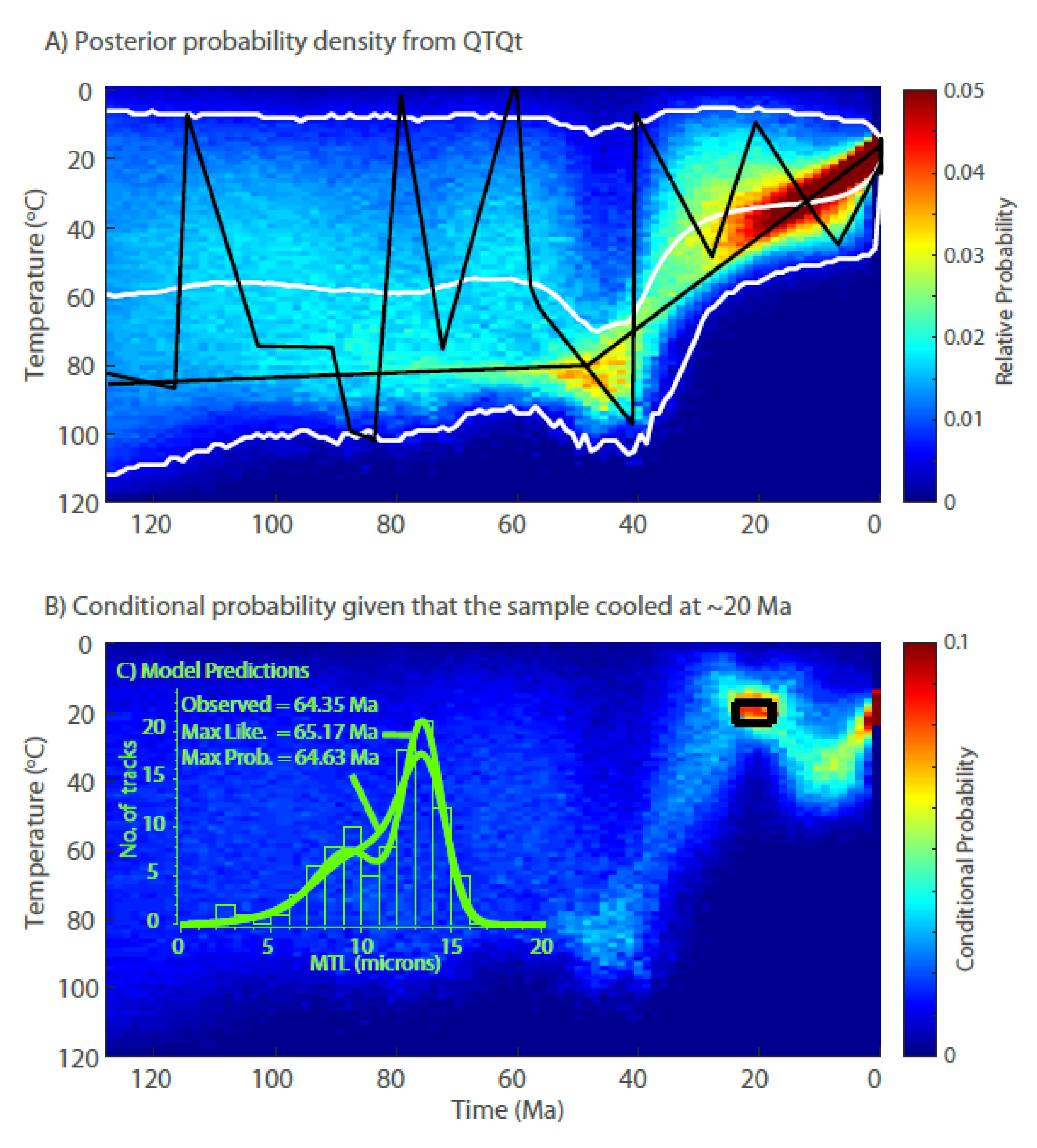
The concept of non-unique models is easiest to explain with thermal history models. Here, we re-interpret data from Gunnell et al. (2007) [47] to illustrate some of these points. These fission track data record the cooling history of rocks from the passive margin of southern Oman where the regional stratigraphy can be used to constrain the margin exhumation history. These rocks were exhumed in the Proterozoic before being buried and re-exhumed following rock uplift and exhumation after rifting between 35 and 18 Ma. We used QTQt to extract a thermal history from sample S9 from this study. The details of the model run can be seen in Figure 5 and the input file for QTQt is provided in the appendix. This inversion nicely demonstrates some of the key issues with reconstructing thermal histories. The best (maximum likelihood) data fitting model (black line in Figure 5A) that QTQt found is very complicated with several inferred stages of burial and reheating. This is not consistent with the relatively simple margin stratigraphy and is therefore, not considered geologically realistic. Nevertheless, it does highlight how non-unique a recovered thermal history is. By contrast, the expected model is shown in white and is much smoother and this is our preferred model in this case as it fits with the geology. Without the independent geological evidence it would be easy to choose a wrong model. The maximum posterior probability model is very simple and does not fit the fission track length data quite as well. We do not show the data fit for the expected model for simplicity but stress that it is important to show this if it is used for interpretative purposes. However, it is important to explore the correlations amongst model parameters. Are there clusters of solutions that share a common characteristic [48]? What is the probability of the rock being at a specific temperature at a specific time if it also has to be at a different temperature at an earlier or later period of time [25]? Here, we demonstrate how the conditional probability can be explored using the output of QTQt in Figure 5B. We explored the correlations amongst model parameters that led to low temperatures at approximately 20 Ma defined with the black box. To do this, we have taken every path that is produced by QTQt that also passes through this box. It is clear that paths that go through this box, also require reheating to maximum temperatures of approximately 40 °C at 10 Ma. Thus, a path that stays at low temperatures over the last 20 Ma, although appearing to be relatively probable, is actually not very probable due to the fact that probabilities are marginals and thus probabilities are dependent on other aspects of the thermal history. Similar assessments of model correlations could be conducted using HeFTy by adding constraint boxes and rerunning the inversion.

Correlations amongst model parameters can be much harder to assess for thermokinematic models. For example, the link between a parameter defining temperature at a fixed depth and a parameter describing exhumation rate may appear obvious: increased geothermal gradients will lead to decreased exhumation rates. However, if the geothermal gradient is also determined by radiogenic heat production, then exhumation during an earlier time period, topographic evolution or variations in lithologically controlled thermal diffusivity through time, cause correlations to become more complicated. It is common to visualize the results of a Pecube inversion using 2D marginal plots that show the correlations amongst pairs of model parameters [35]. By showing lots of these pairs, correlations can be assessed and used to guide the interpretations of the results. Another way to show results is by using a synoptic probability plot [49]. This is a way to collapse groups of model parameters onto a single plot. For example, if exhumation rate is free to vary over varying lengths of time, there may be several model parameters corresponding to the exhumation rate within these intervals and the timings of transitions between different exhumation rate periods. By sampling the parameter space so that the frequency of a specific model parameter being sampled can be related to probability, exhumation rate probability through time can be visualized. Of course, this approach has the same problems that are encountered in thermal history modelling: how many parameters are required? The Bayesian Information Criterion provides a useful way to balance model fit against model complexity and has been used with Pecube models [49]. However, this makes the assumption that the distributions on model parameters are unimodal which is often not the case with high dimensional inverse problems. It is also important to note that in many cases the model complexity can be inferred using geological evidence (e.g., the Oman example above).

For inverse models with thousands of model parameters, the correlation matrices are even harder to assess. For these models, therefore, it is particularly useful to carry out synthetic tests. Synthetic tests should be designed to test a specific component of a model, whether that is the resolution of a specific aspect of the recovered rates or a systematic bias with the method. For example, if the test is designed to test the spatial correlation bias associated with the model parameters, model configuration and the resolution of the data, it should attempt to isolate this. Here, we highlight a simple test designed to isolate smoothing of exhumation rates from ages across a fault. First, we avoid the use of the thermal model and differences in age models by using the ages and the synthetic exhumation rate to define new, imaginary, closure depths. These imaginary closure depths are defined as closure depth equals age times true (synthetic) exhumation rate. In other words, the ages used for this test remain the same so that the spatial and temporal distribution also remains the same. We use the same Alpine study area as Schildgen et al. (2018) [6] and the same model parameters and invert the synthetic imaginary closure depth data. The synthetic ages were produced using Pecube by Schildgen et al. (2018) [6] with one side of a fault exhuming at rates of 1 km/Ma and the other side at rates of 0.1 km/Ma. The data were modelled at the same geographic locations as the Alpine dataset to ensure that spatial distribution of ages was kept constant. We take these synthetic ages and produce imaginary closure depths and then run the inversion. Figure 6A shows that with this dataset, there is considerable smoothing across the fault and this may be a cause of the spatial correlation bias. Even with the perfect, and imaginary, closure depths, GLIDE does not recover the correct solution perfectly [6]. There is, however, no spurious acceleration of erosion rates generated in the last 6 Myr in the high uplift area. The gradient in exhumation from the fault towards the north-east corner of the model domain is due to the lack of ages from this area and the rates are gradually decreasing towards the prior exhumation rate. Next, we take the real Alpine age dataset and produce imaginary closure depths in the same way and run the inversion. Figure 6B, shows that with this dataset, the degree of smoothing across the fault is reduced and that there is again no spurious acceleration in the last 6 Myr. Some smoothing still occurs particularly in the north west corner. This is due to the fact that real ages do overlap either side of the fault. Although the age distribution is suitable to accurately resolve the correct synthetic rates tested here, the distribution may be less suitable for a more complex (and realistic) synthetic test. These two synthetic tests, designed to isolate smoothing across a fault, show that this does occur for the synthetic ages produced by Schildgen et al. (2018) [6], but to a lesser extent for the real ages. This is because although the ages are from the same spatial locations, they are distributed differently in time. Furthermore, because there is no thermal model, different thermal models used in GLIDE and Pecube are not a source of error [50]. We have also highlighted that GLIDE can lead to averaging across faults that may lead to a spatial correlation bias [6] but that the distribution of ages, in space and time, influences the results. Resolution is the formal metric that describes how the true rates are averaged due to the age distribution, age uncertainties, and model, and this is explored in detail in Willett et al. (2020) [50].

In order to resolve some of these debates, it is useful to investigate the models and come up with innovative new data processing paths. These sorts of approaches will help resolve debates around whether there has been an increase in exhumation rate or whether this is an artefact of the thermochronometric methodology and interpretation. OSL-thermochronometry is sensitive to very low temperatures and is thus well suited to provide crucial constraints on recent exhumation rates in rapidly eroding places [51] and may ultimately allow us to test some model predictions. For more slowly exhuming areas, McDannell et al. (2018) [52] provided a rapid quality-screening protocol for (U-Th)/He thermochronometry and there is ongoing work to measure ⁴He/³He in situ [53]. These new analytical tools will need to be integrated into modelling efforts so that age models can be verified and rates more tightly constrained. However, these may be sensitive to different portions of the thermal history and may present challenges in terms of model parameterisations and model resolution. For example, is the uniform prior temperature range commonly used in QTQt suitable for a ZFT age that is millions of years old and an OSL age that is only tens of thousands of years old? Are the model simplifications that are made to heat flow suitable to measure cooling from very shallow depths where fluid flow or Pleistocene climate change may control local geothermal gradients? By developing new interpretative tools with different sets of assumptions and objectives, it is possible to approach problems from new perspectives. Ultimately, this will reduce the dependency on different model assumptions and provide new insight into Earth’s dynamic surface.