Abstract
In Bangkok, the demand for housing is extensively high due to the city growing rapidly, so some swampy areas are filled with soil. A Prefabricated Vertical Drain (PVD) with the Vacuum Consolidation Method (VCM) is required to make the soil applicable for construction. However, it is difficult to monitor the soil strength during the process because the airtight sheet will be broken. This research aims to study the possibility of using the Spectral Analysis of Surface Waves (SASW) test to monitor the effectiveness of the VCM method and to study the development of shear-wave velocity over the consolidation period. Multiple instruments were installed on site, namely, vacuum gauges, settlement plates, and a piezometer, as well as a borehole to monitor the pump pressure, settlement, porewater pressure, and soil properties. Ten SASW tests were taken to measure the change in shear-wave velocity (Vs) over 7 months. The results showed an increment in the Vs along with increments in the settlement and undrained shear strength (Su), as well as a decrement in pore pressure during the consolidation period. The correlation between Vs and soil settlement was developed to predict the amount of settlement using Vs. These all indicated the potential of using the SASW method for soil improvement monitoring purposes.
1. Introduction
In Bangkok, the demand for housing is extremely high due to the city growing rapidly. This raises the question as to where the new housing should be, since most of the area has already been occupied. Some swampy areas were filled with soil to meet this demand. Soil improvement is vital because the backfilled material with its soft soil properties is initially not feasible for construction due to the settlement issue. The function of soil improvement is to increase the soil strength and performance in order to be able to withstand the load applied to the soil due to the construction. One of the examples of the soil improvement method is using a Prefabricated Vertical Drain (PVD) for a faster consolidation rate [1]. Furthermore, a PVD can be applied together with the Vacuum Consolidation Method (VCM) to replace the surcharge load. Many countries have been successfully using this method for land reclamation and soil improvement work [2,3,4,5,6,7]
An airtight sheet is used above the installed PVD area, as an impermeable layer covering the soil surface, allowing both the air and water to be sucked from the ground by the pump [8,9].This airtight-sheet method has successfully been used for vacuum consolidation projects at soil improvement sites [10,11]. The destructive soil test to monitor the soil parameters during the improvement cannot be performed without damaging the sheet itself due to the presence of this airtight sheet. Nevertheless, an in situ, non-destructive test is still an option, and one of the tests is the Spectral Analysis of Surface Waves (SASW) method. This will be the first SASW test to monitor the backfilled soil at the PVD with the VCM at a site in Thailand.
The SASW method is a seismic method utilizing surface waves of the Rayleigh type and has been developed to determine the shear-wave velocity (Vs) and shear modulus profiles of geotechnical sites [12]. The test uses impact sources to produce the surface wave and receivers to retrieve the data. A periodical SASW test is proposed as a method to monitor the development of the soil stiffness overtime. This SASW test will be compared with various field-instrument results to check the compatibility between the SASW test data and other instruments. The objectives of this research are firstly to study the possibility of using the SASW method to monitor the effectiveness of the VCM method; then, to study the development of the shear-wave velocity over the consolidation period; and, lastly, to create a correlation between the Vs and settlement for a VCM settlement prediction based on the Vs.
2. Methodology
2.1. Study Area
The VCM site is located in the north-eastern part of Bangkok, Thailand. It is located on an old pond that has been filled with soil material. Figure 1 shows that the site is divided into 3 zones: Zone A, Zone B, and Zone C. Figure 2 shows the boundary between Zone A and Zone B. In this research, only Zone B that will be monitored with the SASW test. The area of Zone B is approximately 6700 m2 and the original soil at the site was soft Bangkok clay. In the past, approximately a 15-m-thick slice of the original soil was removed, turning the area into a pond. Recently, the pond was backfilled with the soil for construction purposes. On top of the backfilled soil, layers of materials were placed in a particular order, namely, a layer of geotextile, a layer of a 0.5-m-thick sand blanket, another layer of geotextile, and then an airtight-sheet (geomembrane) layer at the very top to cover the surface.
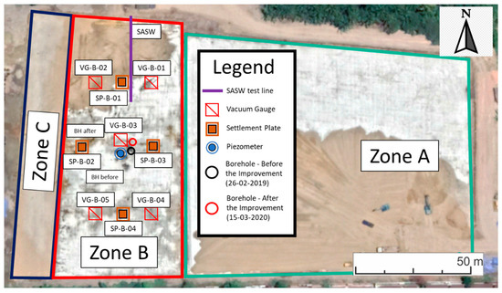
Figure 1.
The overall zone of the Vacuum Consolidation Method (VCM) site and a view of the plan for the instruments’ location in Zone B.
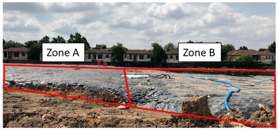
Figure 2.
A photo of Zone A and Zone B, three months after the pumping started (camera facing south).
2.2. Boreholes and Soil Properties
The two boreholes are located approximately 2.5 m apart with different times, from before the soil improvement (26 February 2019) and after the soil improvement (15 March 2020). Boring log data of 30.45 m in Zone B provided information of the soil properties, such as soil strength, Atterberg’s limits, the water content, and the unit weight of soil from a soil sample of 0.5 m long, which was collected at every 1.5 m depth. A thin wall tube and spilt spoon sampler were used for soft clay layer and dense sand layer, respectively. It is worth noting that the backfilled soil was collected from various locations. In this study, however, the soil was assumed to be a homogeneous soil.
Before the pump started, the boring log data had shown that there were 2 layers of the soil profile in Zone B. The first layer ranges from very soft to soft High Plasticity Clay (CH), according to Unified Soil Classification System [13], with a depth of between 0 and 21 m. The second layer was dense to very dense Silty Sand (SM), with a depth of between 21 and 30.45 m (end of borehole). The following soil properties use an average value. For the clay layer, the undrained shear strength (Su) from the Unconfined Compression Test was 9.68 kN/m2, the unit weight 1.6 t/m3, the water content 56.96%, the Liquid Limit 77.33, and the Plastic Limit 27.44. For the sand layer, the (N1)60 value was 25 and water content 19.85%.
After the pump stopped, there were some soil property changes that were observed from the boring log data. From a 1.5 to 4.5 m depth, the strength was increased by 3.5 t/m2, the water content was decreased by 30%, and the unit weight was increased by 0.36 t/m3. From a 4.5 to 21 m depth, the strength was increased by 1.7 t/m2, the water content was decreased by 8.5%, and the unit weight was increased by 0.12 t/m3. From a 21 to 30.45 m depth, there were insignificant changes in the SPT-N value and water content. The summary of the boring log data before and after the soil improvement are shown in Figure 3 and Figure 4.
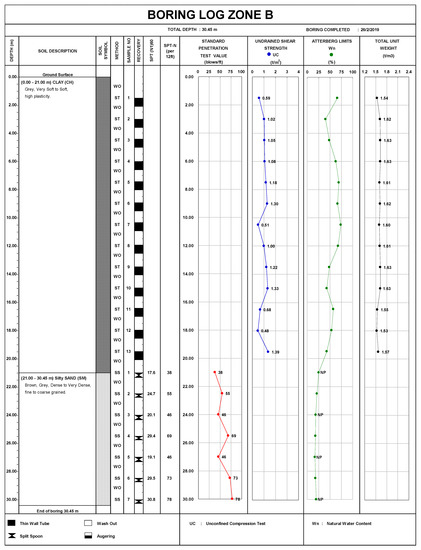
Figure 3.
Summary of Zone B’s boring log data before the soil improvement on 26 February 2019.
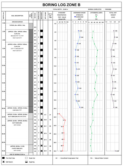
Figure 4.
Summary of Zone B’s boring log data after the soil improvement on 15 March 2020.
Soil properties from the consolidation test results were available from the borehole samples at 3 different depths. From a depth 6 to 6.5 m, the water content was 69.8%, the total unit weight 1.61 t/m3, the preconsolidation pressure 5.6 t/m2, the Cc 1.193, the Cs 0.132, the OCR 1.19, and the Cv 5.09 cm2/sec. From a depth of 12 to 12.5 m, the soil was a normally consolidated clay with a water content of 68.7%, a total unit weight of 1.56 t/m3, a Cc of 0.707, a Cs of 0.083, and a Cv of 2.22 cm2/sec. From a depth of 18 to 18.5 m, the soil was a normally consolidated clay with a water content of 58.1%, a total unit weight of 1.61 t/m3, a Cc of 0.546, a Cs of 0.074, and a Cv of 0.18 cm2/sec.
2.3. VCM, PVD, and Instrumentations
In the early 1950s, Vacuum consolidation was suggested by Kjellman [14]. The PVD and sand drains were used to discharge the pore water and to distribute the vacuum load [15]. The vertical drainage systems significantly reduce the drainage path, consequently accelerating the soil consolidation [16,17,18,19,20]. In this study, the airtight-sheet method was used for the seal system for the vacuum consolidation. A vacuum pump was used with an average pressure of around −80 kPa—continuously during the consolidation settlement process. A PVD was installed in Zone B with an average depth of 14 m with a triangular pattern of a 1.0 m × 1.0 m spacing. The vertical drain penetrated the backfilled soil and the original soil below that. Zone B was instrumented with multiple instruments for monitoring the progress of the soil improvement.
Five vacuum gauges were placed to monitor the sub-surface pressure with a monitoring frequency of once per day. Four settlement plates were placed on the sand blanket below the airtight-sheet layer to observe the soil settlement. There were 3 monitoring plans for the settlement plates. Firstly, for the first month it was one time per day. Secondly, after the first month to the last half month, it was two times per week. Thirdly, for the last half month it was one time per day. A piezometer with a vibrating wire sensor was placed at a depth of 8.5 m at the center of Zone B to observe the change in porewater pressure over time. Figure 1 also shows the locations of the instruments.
2.4. The SASW Test
Surface waves were used by [21,22], one of the first researchers who tried to examine pavement systems. The engineers were able to build more advanced tools and equipment due to the advancement of technology. Because of these new tools, researchers were able to perform better and more accurate calculations in very little time. Provided with the new, advanced equipment, [23] was able to change from the empirical to the theoretical level regarding the surface wave method.
SASW is an in situ, low strain, non-destructive test. which has successfully been implemented by researchers of the University of Texas at Austin, as well as other researchers, to investigate the Vs and shear modulus of many pavements and highway materials [24,25,26] and to predict the long-term settlement based on the Vs and damping characteristics [27]. In Thailand, many SASW tests were implemented at several dams for material stiffness examination [28,29,30,31], measuring the Vs of a dyke and liquefaction site [32,33,34], as well as investigating the small strain modulus of the silty sand subgrades [35].
In this research study, a series of SASW tests were conducted 10 times in a 7-month period—before the pumping of the VCM started until the pump was shut down; this was the time necessary for the soil settlement to reach the desired target. The frequency of the SASW testing was twice a month for the first two months and once a month after that. The test repetition was set in such conditions as the soil settlement was expected more at the beginning of the consolidation settlement.
The SASW test used receiver spacings of 0.5, 1, 2, 4, 6, 12, and 20 m. This study used 2 different configurations of the SASW test, namely, the common source array test configuration and common receiver mid-point configuration, which are shown on Figure 5. For receiver spacings of 12 and 20 m, the tests were conducted with the former test configuration, while the rest of the spacings were conducted with the latter test configuration. There are three impact sources used in this study, as shown in Figure 6. A 300 kg drop weight was used for far receiver spacings, to generate a low frequency wave to investigate the deep profile, but can only be dropped on the soil outside of Zone B to prevent this from damaging the airtight sheet in Zone B. A 25 kg small drop weight and a sledgehammer were used for the intermediate and short spacings and can be used on top of the airtight sheet to preserve the membrane itself. Since the original backfilled soil was very soft, the sledgehammer could not generate sufficiently high energy for the receiver spacings larger than 4 m without breaking the air-tight sheet; hence, the 25 kg small drop weight, which can generate higher energy, was used for the intermediate spacings instead. Two 2-Hz geophones were used as the receivers. The procedure for the SASW test consisted of the following: firstly, to acquire the data from the field that were collected by the spectrum analyzer, and then to analyze the dispersion curves and shear-wave velocity profile using the WinSASW program developed by Joh in 1996 [36].
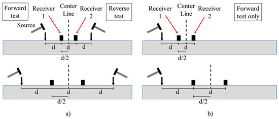
Figure 5.
Two different test configurations conducted in this research: (a) the common receiver mid-point; (b) the common source.
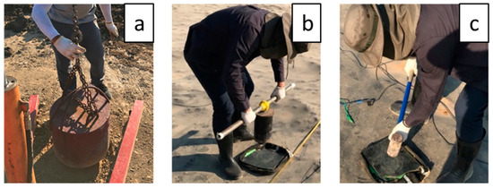
Figure 6.
The impact sources of the Spectral Analysis of Surface Waves (SASW) test: (a) a 300 kg drop weight for far spacing; (b) a 25 kg drop weight for intermediate spacing; (c) a sledge hammer for short spacing.
The SASW test centerline was located as nearly as possible to a borehole location in Zone B in order to be able to compare both test data sets. The 300 kg heavy drop weight cannot be dropped on the surface of Zone B as mentioned above and, therefore, the heavy drop weight can only be dropped outside of Zone B and from the edge of the zone as nearly as possible, so the centerline of the SASW test is approximately 30 m away from the borehole location. It is worth noting that the centerline of the 12 m spacing was different from the rest of the spacing for a similar reason as above. The SASW centerline sometimes shifted in the vicinity of 5 m due to some submerged water area being trapped on top of the membrane after rain. The duration of the SASW test varied between 30 min to 1 h; the increasing amount of time was because of the noise presented at the site. A lot of construction machinery was operating and creating noises and was captured by the geophones, rendering the data unusable. The test must be repeated or even stopped until the source of the noises was cleared.
An average shear-wave velocity of 15 m deep of the improved soil (Vs15) was used as the monitoring parameter because the Vs can be different at each depth and the approximate PVD length was 14.7 m. The Vs15 can be calculated by the following formula adapted from the Vs30, which was used in the National Earthquake Hazards Reduction Program (NERHP) for site classification [37]:
where hx and vx represent the thickness (in meters) and shear-wave velocity (in m/s) of the xth layer, in a total of N, existing in the top 15 m.
3. Results and Discussion
3.1. SASW Result
Figure 7 shows the Vs profiles for Zone B over the consolidated time. The first test was on the 30th of July 2019, before the pump started, and the last test was on the 2nd of March 2020, after the pump stopped. The increment in Vs was noticeable over time. The top layer was the sand blanket with a thickness of approximately 0.5 m, showing a high value of Vs. The middle layer was the very soft soil with an approximate thickness of 10 m, showing a low value of Vs. The bottom layer was the soil with a higher Vs from the layers before. Since the first test to the last, the Vs has changed around 40 m/s at the top layer and middle layer, and around 70 m/s at the bottom layer. The top layer has the highest value of Vs because it is a sand blanket that was affected the most by the vacuum pressure from the pump. On the other hand, the bottom layer has a high value of Vs, potentially because of a high overburden pressure from the upper layer. Note that the Vs profile was measured from the ground surface and the actual ground level at each time is different from the initial ground level due to the settlement over time.
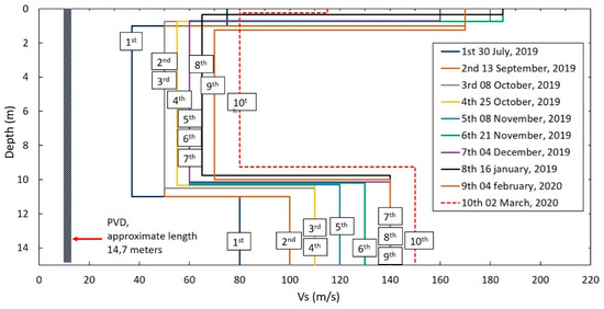
Figure 7.
The Vs profile of the Zone B at different times, from before the start of the pumping until after the pumping stopped.
3.2. Comparison of Settlement and Vs
The result from the settlement plates was recorded to determine the change in the soil settlement. The settlement plate of SP-B-01 was used since the location was the closest to the SASW test line. The initial SASW test was performed around 3 weeks before the installation of the PVD in the field. Figure 8 shows the changing of the settlement and Vs15 over time. The Vs15 increased with the increasing settlement of soil as the soil became denser during the consolidation process. While the settlement is faster at the beginning and then starting to slow down through the end, the total settlement was 1.12 m. In contrast, the development of the Vs shows a steady increment over time, with the maximum deviation from the “linear” trend line being 6.14 m/s.
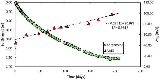
Figure 8.
Comparison between the settlement and Vs15 over time.
Figure 9 shows the correlation between settlement and the Vs15. The correlation between settlement and the Vs15 is well-suited with a straight trendline, where the Vs15 increases gradually with the increasing settlement over time. The settlement roughly increased 0.25 m for every 10 m/s increment in Vs15. An equation was made from this correlation to predict the amount of settlement by the value of the Vs15. The equation can be written as
where s stands for settlement (in meter).
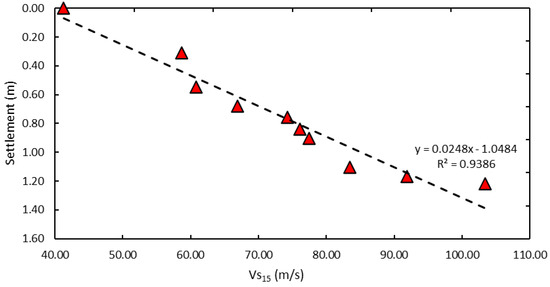
Figure 9.
Relationship between settlement and Vs15.
The field measurement result was then compared with the theoretical model of settlement prediction from [38] and with a back-analysis model of the Vs15 from the SASW test, as shown in Figure 10. The model of [38] was commonly used for settlement prediction, with the time based on the measured settlement data. The prediction was based on an observational procedure and derived from a 1-dimensional consolidation equation. Vertical strain can be calculated as follows:
where ε(t,z) is the vertical strain of depth z at time t, T and F are unknown functions of time, and Cv is the coefficient of consolidation.
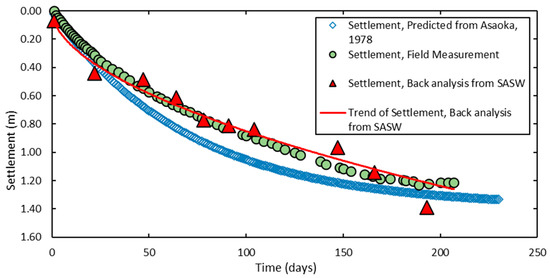
Figure 10.
Settlement curve.
The equations of settlement for double drainage can be written as in the following formula:
where ρ is settlement, H is soil thickness, and is the vertical strain at its initial time.
Each individual time can be expressed as
where ∆t is the time interval.
From Equations (4) and (5), the settlement equation at time j can be calculated as follows:
where ρj and ρj−1 are the value of settlement at the specific time of j and j − 1; β0 and β1 are unknown parameters.
The final settlement can be calculated using the following formula:
where ρf is the final settlement.
The final settlement can be predicted by finding the intersection from the line ρj and ρj−1, which has a 45° angle from the ρj and ρj−1 graph. Based on this, Equation (6) can be simplified by substituting ρj and ρj−1 with ρf and can be written as
And finally, the settlement ρ(t) at specific time t can be predicted by the following formula:
where ρ0 is the value of the settlement at its initial time.
The result from the back-analysis of the Vs15 prediction is very close to the field measurement settlement, with the range of deviation being between 0.004 and 0.070 m, as well as to the result taken from the predicted settlement from [38], with the range of deviation being between 0.002 to 0.202 m.
3.3. Comparison of Pore Pressure and Vs
The result of pore pressure was obtained from the piezometer installed at a depth of 8.5 m (in the middle of the improved soil layer) at the center of the study zone. Figure 11 shows the change in pore pressure over time versus Vs at the 8.5 m depth over time. The pore pressure decreased because the water dissipates out of the soil through the PVD, making the soil stiffer, which, in turn, increases the Vs. Both pore pressure and Vs are nicely suited as both parameters increase linearly over time. Unlike the SASW test, the pore pressure data from the piezometer was monitored roughly 1 time per day while the SASW tests were performed only 10 times during the settlement period, about 7 months since the pump had been started until it was stopped.
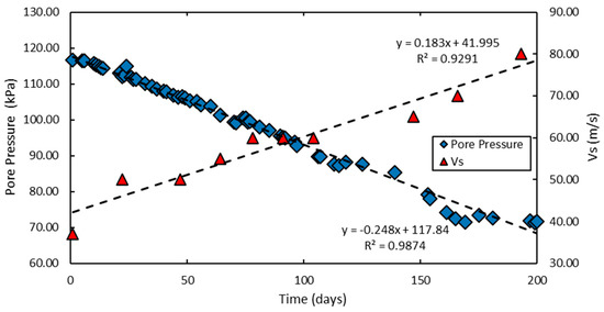
Figure 11.
Pore pressure and Vs. Vs over time at a depth of 8.5 m.
Additionally, the effective vertical stress was calculated from the change in pore pressure over time. Figure 12 shows the correlation between effective vertical stress and Vs at a 8.5 m depth. The Vs had linearly increased along with the increase in the effective vertical stress as the pore pressure dissipated out and made the soil stiffer.
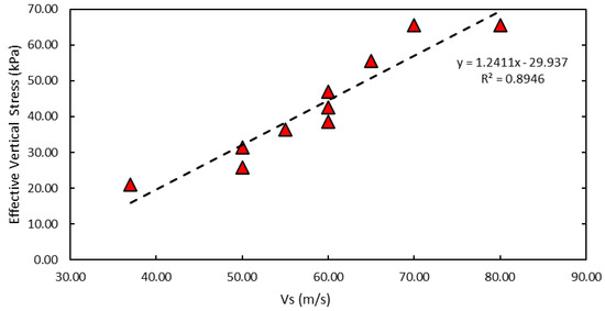
Figure 12.
The relationship between effective vertical stress and Vs15 at a depth of 8.5 m.
3.4. Comparison of Su and Vs
The Su data were acquired from an unconfined compression test of undisturbed soil samples collected from bore holes from two different times, before the soil improvement (26 February 2019) and after the soil improvement (15 March 2020). It is worth noting that the Vs values that were used for the comparison were the ones measured from the closest times to the Su measurements. Figure 13 shows the comparison between Su and Vs at those times. After the pump had stopped, Su from the first 5 m range increased significantly to an approximate of 30 kN/m2, considering the stress distribution of the atmospheric pressure is higher at the top layer than the layer below. At the middle part of the soil, from 5 to 9 m depth, the Su values increase only to an approximate of 7 kN/m2. At the bottom part of the soil, from 9 to 15 m depth, the Su values increase approximately 15 kN/m2. The Su of the bottom part of the soil layer increases potentially more than the middle part due to the higher overburden pressure and dissipation of water to the sand layer below.
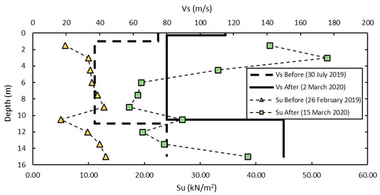
Figure 13.
Su and Vs from before the soil improvement and after the soil improvement.
The SASW data shows an increment at the top of the layer, the sand blanket, of approximately 40 m/s. In the middle part of the soil, from 1 to 11 m depth, the Vs increase around 40 m/s in comparison with the initial Vs number. At the bottom part of the soil, from 11 to 15 m depth, the Vs increase around 70 m/s. It is noticeable that the increment in Vs at the bottom part of the soil layer is higher than the middle part, which is similar to the increment in Su due to similar reasons.
4. Conclusions and Recommendations
The change in Vs and soil properties were studied over time during the VCM process. The SASW testing was able to investigate the soil down to 15 m deep. The results showed the change in Vs along with the alteration of the conventional soil monitoring parameters, including the settlement, Su, and pore pressure during the consolidation period. The Vs15 had increased linearly from 45 m/s to 98 m/s from the beginning until the end of the consolidation process, while the total settlement was 1.12 m, Su increased about 7 to 15 kN/m2, and the pore pressure decreased about 40 kPa. The settlement prediction curve using Vs was created and good compatibility was shown with the settlement curve from field measurements and the settlement prediction curve from [35]. These results indicated the likelihood of using the SASW method for soil improvement monitoring purposes.
There were several difficulties of testing SASW at the PVD sites. Firstly, the location of the SASW center line and borehole data location is different as the 300 kg drop weight could not be used on top of the airtight-sheet region. Secondly, sometimes the test line was shifted within the range of 5 m knowing that the water is being trapped at the testing spot after rain. Thirdly, the presence of noises in the field from a moving truck to a working backhoe, which creates poor quality data, meant that the operations on site had to be interrupted during the SASW test in order to improve the quality of the data. It is important to note that the correlation was made from backfilled soil material that was characterized by high plasticity clay and an assumption of homogenous soil. The study of other soil types is encouraged.
Author Contributions
Conceptualization, D.F.A., S.C. and S.S.; data curation, D.F.A.; formal analysis, D.F.A. and S.C.; funding acquisition, S.C. and S.S.; investigation, D.F.A. and S.C.; methodology, D.F.A., S.C. and S.S.; project administration, D.F.A., S.C. and S.S.; resources, S.C. and S.S.; supervision, S.C. and S.S.; validation, S.C. and S.S.; visualization, D.F.A., S.C. and S.S.; writing—original draft, D.F.A. and S.C.; writing—review and editing, S.C. and S.S. All authors have read and agreed to the published version of the manuscript.
Funding
The scholarship was provided by the Faculty of Engineering, Kasetsart University (KU), Bangkok, Thailand.
Acknowledgments
The authors appreciate the scholarship provided by the Department of Civil Engineering, Faculty of Engineering, KU, Bangkok, and they are grateful to the graduate students and the staff members of the Geotechnical Division and Geotechnical Engineering Research and Development Center (GERD) of KU and SILA GEOTECHNIQUE Co., Ltd. for the support and opportunity that has been given in this research project.
Conflicts of Interest
The authors declare no conflicts of interest.
References
- Budhu, M. Soil Mechanics and Foundation, 3rd ed.; John Wiley & Sons Inc.: Hoboken, NJ, USA, 2010; pp. 246–249. ISBN 978-040-55684-9. [Google Scholar]
- Holtz, R.D.; Wager, O. Preloading by Vacuum: Current Prospects. Transp. Res. Rec. 1975, 548, 26–29. [Google Scholar]
- Chen, H.; Bao, X.C. Analysis of Soil Consolidation Stress under the Action of Negative Pressure. In Proceedings of the 8th European Conference on Soil Mechanics and Foundation Engineering, Helsinki, Finland, 23–26 May 1983; pp. 591–596. [Google Scholar]
- Choa, V. Soil Improvement Works at Tianjin East Pier project. In Proceedings of the 10th Southeast Asian Geotechnical Conference, Taipei, Taiwan, 16–20 April 1990; pp. 47–52. [Google Scholar]
- Jacob, A.; Thevanayagam, S.; Kavazanjian, E. Vacuum-assisted Consolidation of a Hydraulic Landfill. In Proceedings of the Conference on Vertical and Horizontal Deformations of Foundations and Embankments Part 2 (of 2), College Station, TX, USA, 16–18 June 1994; pp. 1249–1261. [Google Scholar]
- Bergado, D.T.; Chai, J.C.; Miura, N.; Balasubramaniam, A.S. PVD Improvement of Soft Bangkok Clay with Combined Vacuum and Reduced Sand Embankment Preloading. Geotech. Eng. J. 1998, 1, 95–122. [Google Scholar]
- Chu, J.; Yan, S.W.; Yang, H. Soil Improvement by the Vacuum Preloading Method for an Oil Storage Station. Geotechnique 2000, 6, 625–632. [Google Scholar] [CrossRef]
- Chai, J.C.; Carter, J.P. Deformation Analysis in Soft Ground Improvement; Springer: Dordrecht, The Netherlands, 2011. [Google Scholar]
- Chai, J.; Carter, J.P.; Liu, M.D. Methods of Vacuum Consolidation and Their Deformation Analyses. Proc. Inst. Civ. Eng. Ground Improv. 2014, 1, 35–46. [Google Scholar] [CrossRef]
- Wahyu, A.L.; Mochtar, I.B. The Effectiveness of Vacuum Preloading on Eliminate Secondary Settlement; Case Study in Summarecon City Bandung Area’s Development Project. In Proceedings of the IOP Conference Series: Earth and Environmental Science, Makassar, Indonesia, 1–2 November 2018; Volume 279, p. 012023. [Google Scholar]
- Phakdimek, S.; Soralump, S. Pore Pressure Behavior of Clayey Backfilled Soil in a Pond Improved by Vacuum Consolidation Method. In Proceedings of the 8th Regional Symposium on Infrastructure Development in Civil Engineering (RSID8), Quezon City, Philippines, 25–26 October 2018. [Google Scholar]
- Stokoe, K.H.; Wright, S.G.; Bay, J.A.; Roesset, J.M. Characterization of Geotechnical Sites by SASW Method, Technical Report: Geophysical Characterization of Sites; Woods, R.D., Ed.; Oxford and IBS Publishing Co.: New Delhi, India, 1994; pp. 15–25. [Google Scholar]
- ASTM. Test Method D2487/D2487-17, Standard Practice for Classification of Soils for Engineering Purposes (Unified Soil Classification System); ASTM International: West Conshohocken, PA, USA, 2017. [Google Scholar]
- Kjellman, W. Consolidation of Clayey Soils by Atmospheric Pressure. In Proceedings of the Conference on Soil Stabilization, Massachusetts Institute of Technology, Boston, MA, USA, 18–20 June 1952; pp. 258–263. [Google Scholar]
- Chu, J.; Yan, S.W. Application of the Vacuum Preloading Method in Soil Improvement Project. In Elsevier Geo-Engineering Book Series; Elsevier: Amsterdam, The Netherlands, 2005; Volume 3, pp. 91–117. [Google Scholar]
- Hansbo, S. Consolidation of Fine-grained Soils by Prefabricated Drains and Lime Column Installation. In Proceedings of the 10th International Conference on Soil Mechanics and Foundation Engineering, Stockholm, Sweden, 15–19 June 1981; pp. 677–682. [Google Scholar]
- Indraratna, B.; Redana, I.W. Numerical Modeling of Vertical Drains with Smear and Well Resistance Installed in Soft Clay. Can. Geotech. J. 2000, 37, 133–145. [Google Scholar] [CrossRef]
- Bergado, D.T.; Balasubramaniam, A.S.; Jonathan, F.R.; Holtz, R.D. Prefabricated Vertical Drains in Soft Bangkok Clay: A case study of the new Bangkok International Airport project. Can. Geotech. J. 2002, 39, 304–315. [Google Scholar] [CrossRef]
- Indraratna, B.; Bamunawita, C.; Khabbaz, H. Numerical Modelling of Vacuum Preloading & Field Applications. Can. Geotech. J. 2004, 41, 1098–1110. [Google Scholar]
- Chai, J.C.; Hong, Z.S.; Shen, S.L. Vacuum-Drain Method Induced Pressure Distribution and Ground Deformation. Geotext. Geomember. 2010, 28, 525–535. [Google Scholar] [CrossRef]
- Jones, R. Surface Wave Technique for Measuring the Elastic Properties and Thickness of Roads: Theoretical Development. Br. J. Appl. Phys. 1962, 13, 21–29. [Google Scholar] [CrossRef]
- Heukelom, W.; Klomp, J.G. Dynamic Testing as a Means of Controlling Pavements During and After Construction. In Proceedings of International Conference on Structural Design of Asphalt Pavements; University of Michigan: Ann Arbor, MI, USA, 1962; pp. 495–510. [Google Scholar]
- Nazarian, S. In Situ Determination of Elastic Moduli of Soil Deposits and Pavement Systems by Spectral-Analysis-of-Surface-Waves Method. Ph.D. Thesis, The University of Texas, Department of Civil Engineering, Austin, TX, USA, 1984. [Google Scholar]
- Nazarian, S.; Stokoe, K.H. In Situ Determination of Elastic Moduli of Pavement Systems by Spectral-Analysis-of-Surface-Waves Method: Practical Aspects; Research report 368-1F; The University of Texas at Austin: Austin, TX, USA, 1985; 161p. [Google Scholar]
- Nazarian, S.; Stokoe, I.; Kenneth, H.; Briggs, R.C.; Rogers, R. Determination of Pavement Layer Thicknesses and Moduli by SASW Method. Transp. Res. Rec. 1988, 1196, 133–150. [Google Scholar]
- Ismail, M.; Samsudin, A.; Rafek, A.; Nayan, K. Road Pavement Stiffness Determination Using SASW Method. Unimas E J. Civ. Eng. 2012, 3, 9–16. [Google Scholar] [CrossRef]
- Omar, M.N.; Abbiss, C.P.; Taha, M.R.; Nayan, K.A.M. Prediction of Long-Term Settlement on Soft Clay using Shear Wave Velocity and Damping Characteristics. Eng. Geol. 2011, 4, 259–270. [Google Scholar] [CrossRef]
- Bay, J.A.; Chaiprakaikeow, S. Spectral Analysis of Surface Waves (SASW) testing of Srinagarind and Vajiralongkorn Dams. In Electricity Generating Authority of Thailand (EGAT) Report, Bangkok, Thailand; Electricity Generating Authority of Thailand: Nonthaburi, Thailand, 2006. [Google Scholar]
- Bay, J.A.; Chaiprakaikeow, S. Spectral Analysis of Surface Waves (SASW) testing of Sirikit and Rajjaprabha Dams. In Electricity Generating Authority of Thailand (EGAT) Report, Bangkok, Thailand; Electricity Generating Authority of Thailand: Nonthaburi, Thailand, 2009. [Google Scholar]
- Chaiprakaikeow, S.; Bay, J.A.; Chaowalittrakul, N. Study of Dynamic Properties of Mae Chang Dam Using Spectral Analysis of Surface Waves and Resonance Tests. In Proceedings of the 21th National Convention on Civil Engineering, Songkla, Thailand, 28–30 June 2016; p. 1426. [Google Scholar]
- Chaiprakaikeow, S.; Bay, J.A.; Chaowalittrakul, N.; Brohmsubha, P. Evaluation of the Effect of Concrete Blocks on Seismic Response of Bhumibol Dam Using In-Situ Dynamic Tests. In Proceedings of the 85th Annual Meeting of International Commission on Large Dams (ICOLD2017), Prague, Czech Republic, 3–7 July 2017. [Google Scholar]
- Mase, L.Z.; Likitlersuang, S.; Tobita, T.; Chaiprakaikeow, S.; Soralump, S. Local Site Investigation of Liquefied Soils Caused by Earthquake in Northern Thailand. J. Earthq. Eng. 2018, 22, 1–24. [Google Scholar] [CrossRef]
- Jotisankasa, A.; Pramusandi, S.; Nishimura, S.; Chaiprakaikeow, S. Field Response of an Instrumented Dyke subjected to Rainfall. Geotech. Eng. J. SEAGS AGSSEA 2019, 50, 81–91. [Google Scholar]
- Shrestha, A.; Jotisankasa, A.; Chaiprakaikeow, S.; Pramusandi, S.; Soralump, S.; Nishimura, S. Determining Shrinkage Cracks Based on the Small-Strain Shear Modulus–Suction Relationship. Geosciences 2019, 9, 362. [Google Scholar] [CrossRef]
- Barus, R.M.N.; Jotisankasa, A.; Chaiprakaikeow, S.; Sawangsuriya, A. Laboratory and Field Evaluation of Modulus-Suction-Moisture Relationship for a Silty Sand Subgrade. Transp. Geotech. 2019, 19, 126–134. [Google Scholar] [CrossRef]
- Joh, S.H.; Stokoe, K.H. Advances in Interpretation and Analysis Techniques for Spectral-Analysis-of-Surface-Waves (SASW) Measurements; Offshore Technology Research Center: College Station, TX, USA, 1997. [Google Scholar]
- BSSC. NEHRP Recommended Provisions for the Development of Seismic Regulations for New Buildings, Part I: Provisions, Building Seismic Safety Council; Federal Emergency Management Agency: Washington, DC, USA, 1994.
- Asaoka, A. Observational Procedure of Settlement Prediction. Soil Found. 1978, 4, 87–101. [Google Scholar] [CrossRef]
© 2020 by the authors. Licensee MDPI, Basel, Switzerland. This article is an open access article distributed under the terms and conditions of the Creative Commons Attribution (CC BY) license (http://creativecommons.org/licenses/by/4.0/).