Abstract
Net fences are among the most widespread passive protective measures to mitigate the risk from rockfall events. Despite the current design approach being based on partial safety factors, a more efficient time-dependent reliability approach has been recently introduced by the authors. This method is influenced by various parameters related to the geometry and the kinematics of the block, i.e., the uncertainty related to the distribution of the size of the impacting block, its occurrence probability, and the shape of the right-tail of the distributions of its velocity and trajectory height at the location of the net fence. Furthermore, the block size distribution of the deposit greatly affects the results. The present work focuses on the possible range of such parameters to encompass the great majority of real events. The obtained results are compared with the current design approaches based on fixed partial safety factors. It emerges that the choice of the characteristic mass of the block and the failure probability greatly influence the results. Moreover, if a set of partial safety factors is assigned to different sites, an intrinsic variability in the failure probability has to be accepted. Suggestions for an accurate procedure and future developments are provided.
1. Introduction
Rockfalls are among the most hazardous landslide phenomena, due to their abrupt occurrence and the very high involved energies [1,2,3,4]. Consequently, effective mitigation measures are required for reducing the hazard and, thus, the risk. This need especially holds for high valuable and vulnerable elements at risk as transportation routes [5,6,7], railways [8] or even urban settlements [9]. In recent decades, the knowledge and the technology on passive mitigation measures have been significantly improved, with particular reference to rockfall flexible barrier, also called net fences [10,11]. A considerable number of new devices and assembly methods have been designed, differing not only for the resistant static scheme and the way of dissipating and transferring impact loads [12,13,14], but aiming also at increasing the effectiveness of the protection and the efficiency during the expected working life [15]. Since the eighties, net fences have been considered as protection kits, whose performance has to be assessed in relation to their essential characteristics, e.g., energy absorption capacity, height, and maximum elongation [16,17]. For this purpose, a European codified method for the assessment of net fences as rockfall protection kits was developed, first in ETAG 027 [18] (”Guideline for European Technical Approval of Falling Rock Protection Kits”), and now in EAD 340059-00-0106 [19] (“Falling Rock Protection Kits”).
The common design relies on a performance based procedure. In other words, from the results of the rockfall propagation analyses, an appropriate commercial product is selected [17] among the ones whose energy absorption capacity and the nominal height, evaluated with standard procedure [19], are greater than the correspondent impact energy and passing height of the simulated blocks. This approach considers two possible failure modes: the falling block trajectory is higher than barrier height, or because its energy is larger than the barrier capacity. Nevertheless, the procedure does not directly consider the impacting conditions, e.g., the position and the angle of impact with respect of the net or the posts, as well as the shape of the impacting block [20,21]. To encompass all these uncertainties, each protection kit is classified according to energy absorption categories. More complex analyses and studies, performed through FEM (Finite Element Method) or DEM (Discrete Element Method) modelling approaches [22,23,24,25,26,27,28], provide an enhancement in understanding the dynamic interaction between the block and the structure, and the transfer load process. Nonetheless, these computationally demanding approaches offer profitable solutions for the design of more efficient devices or the assembly of the single components, resulting more useful for the producer rather than being affordable for the designer. Similarly, meta-models techniques [21,29] requiring outputs derived from either accurate numerical models or experiments are tailored on specific products and, hence, can be inconvenient for general design purposes.
At the base of any modern design code, such as the European standards EN 1990:2002 [30], the design value of the effects of the action has to be lower or equal to the design value of the effects of the resistance . The standardised performance-based design procedure defined within the national recommendations UNI 11211-4 [31] in Italy and ONR 24810 [32] in Austria suggest to evaluate the design parameters of the actions from a single characteristic value of the distribution of the impacting energy (or velocity) and height, resulting from the trajectory analyses [10,33,34,35]. In the framework of the previously mentioned national recommendations, these design values are the product between characteristic values and partial safety factors. In particular, the UNI 11211-4 [31] considers the 95th percentile of the distribution for both velocity and height, and the related partial safety factors depend on the quality of the adopted trajectory model type and input parameters. The characteristic value of the impacting block mass is defined as a percentile (95th or larger) of the distribution of the masses. The ONR 24810 [32] adopts the 99th percentile for the energy and the 95th for the height, and the partial safety factors are related with the occurrence probability of a rockfall event and the consequence class of the elements at risk. A distribution of possible falling blocks has to be defined and a percentile of this distribution has to be considered as the characteristic value.
Some critical aspects in the application of the European standards EN 1990:2002 [30] for the design of rockfall net fences have been recently highlighted and fixed through a time-integrated reliability based approach [36]. Choosing a suitable failure probability, the design kinetic energy and passing height of the impacting block are determined from the results of the performed trajectory analyses. The reliability approach allows to consider the random nature of the parameters affecting the performance and the safety of a system [37] providing, in this specific case, probability distributions of the parameters of the impact and, theoretically, of the resistance. The method also accounts for the variability in the magnitude and the temporal occurrence probability of an impact, which are thoroughly site specific [1,38,39].
In a tentative to merge the time-integrated reliability based approach with the current practice, the calculation can be simplified by considering the values of the CE certified maximum energy level absorption capacity (MEL) , the nominal height , and the tolerance t as Dirac- distributions [36]. If more information derived from field tests or numerical modelling would be available, different probability distributions could be assigned to the variables. With the aim of providing a compelling solution for the designer, De Biagi et al. [36] implemented their approach into the current practice [30]: equivalent partial safety factors for the impacting block energy, mass, velocity, and height were derived, and properties and the affecting variables were analysed.
Starting from the evidence that rockfall phenomena are extremely variable in terms of magnitude and kinematics, i.e., type and direction of motion, velocities, and height, in the present paper the Authors investigate the possible scenarios which can occur in a real case. The results lead to the identification of a range of values of partial safety factors for each of the two failure modes.
The paper is structured as follow. Section 2 summarises the reliability-based design approach, considering the possible failure mechanisms. Section 3 explains the adopted procedure to investigate all the possible rockfall scenarios, while the results of the parametric analyses are introduced in Section 4. Section 5 provides an attempt to find a range of values of partial safety factors to adopt. Finally, the suggestions and future possible development are discussed in Section 6.
2. Basics of Reliability of Rockfall Protection Structures
As mentioned in Section 1, the possible failure modes can be related to the height and the energy of the impacting block, which can be higher than the barrier intercepting height and absorption capacity . Lower case stands for block, while capital for the barrier. The failure probability of the system can be considered as the sum of the failure probabilities related to each of the two scenarios, i.e., and , for excessive height and for excessive kinetic energy, respectively. The failure probability is assumed to be equal to the probability that a block has a trajectory higher than barrier height, disregarding its kinetic energy. Similarly, the failure probability is assumed to be equal to the probability that a block impacts with a kinetic energy greater than the barrier capacity, disregarding its height. This assumption allows to obtain a conservative value of and, thus, a precautionary design procedure [36].
Each failure mode accounts for a specific failure scenario, which can be mathematically described through a limit function representing the boundary between failure and safety, through which the reliability can be assessed. The two limit functions are derived as solutions, i.e., imposing to zero, of a state functions, which describe if the system is in a safe or unsafe condition. For a specific value of the reliability, i.e., a failure probability, the design values of the variables (denoted with subscript ) composing the state function are obtained.
The proposed approach is time-integrated, considering that all the statistical properties of the variables have to be related to a time period. This is particularly important since the possible rockfall impacting impacting mass is associated to a temporal occurrence. According to De Biagi et al. [36], for a given return period T, it is assumed that the mass is normally distributed with a mean value computed through a power-law rule, as suggested in [40]:
where represents the shape coefficient of a Pareto Type I distribution and accounts for the heterogeneity of the size of the blocks, is the threshold mass whose occurrence frequency is . The spread of the distribution is determined through the coefficient of variation, , i.e., the ratio between the standard deviation and the mean value.
2.1. Failure Due to Excessive Height
This section deals with the failure due to excessive height. In the proposed approach, the state function accounting for the exceeding of the barrier height, , is [36]:
where is the height of the trajectory in the position in which a net fence is supposed to be installed, and t is the tolerance due to the block size [31], considering that is measured in the centre of mass of the impacting block. The failure probability , related to height state function, is computed as:
where is the joint probability density function of the trajectory, of the barrier height, and of the tolerance. This expression is consistent with a lumped-mass assumption for the trajectory analyses, i.e., absence correlation between the size of the falling block and its trajectory. The failure probability due to excessive height during the period of analysis , e.g., the lifetime of the system or one year, is obtained as [36]:
where is the mean rate of occurrence of an event, which can be assumed equal to . As already mentioned, a Dirac- distribution at the value of the CE (marking) certified nominal height is assumed. For sake of simplicity, the same assumption holds for the tolerance t.
2.2. Failure due to Excessive Kinetic Energy
The failure due to excessive kinetic energy has to account for the variability of the impacting block size, which differs from event to event. The relationship between the rockfall block mass, to which the kinetic energy is proportional, and its temporal frequency, i.e., its return period T, is expressed by Equation (1).
Given the occurrence of an event, the probability of failure due to excessive kinetic energy considers that the maximum energy depends on the occurrence of certain values of the mass and of the velocity, chosen inside their probability distributions as representative (or characteristic) as [36]:
where is the joint probability density function of the characteristic values of the mass and the velocity, defined through the random variables and , respectively. Under the lumped-mass assumption, the velocity and the mass are independent and, thus, the joint probability density function is the product of the single probability density functions, i.e., and . Since the lumped-mass propagation analysis outputs a single distribution of the velocities, the characteristic value of the velocity is unique: is a Dirac- distribution at . Hence, Equation (5) turns into:
Conversely, for each return period T a normal distribution centred in the mean value computed through Equation (1) can be evaluated, and the probability density function related to the characteristic value of the mass, variable with T, can be described through a Pareto Type I distribution according to De Biagi et al. [39] as:
The conditional failure probability is studied introducing the state function accounting for the exceeding of barrier energy capacity , expressed as:
where m and v are the impacting block mass and velocity, respectively. The conditional failure probability related to the state function is computed as:
where is the joint probability density function of the mass (with a characteristic value equal ) the velocity of the impacting block, and the capacity of the barrier. As reported in [36], the failure probability in the chosen time period due to excessive kinetic energy is obtained as:
As in Equation (4), can be assumed equal to .
2.3. From the Reliability Design Approach to the Semi-Probabilistic Method: Equivalent Partial Safety Coefficients
Similarly for other structural engineering design problems, the reliability approach can be alternatively considered both for the design, and, for a given reliability, for finding the partial safety factors to be adopted in the current semi-probabilistic methods (code calibration procedure [37]). In the present problem, three partial safety factors, namely, , and , can be defined. The safety factors are the ratios between the design values of the parameter and their characteristic values referred with the subscript , in accordance with EN 1990:2002 [30]. Referring to the Italian recommendation UNI 11211-4 [31], the 95th percentiles of velocity and passing height are considered as characteristic values, i.e., and . To evaluate the partial safety factor it is necessary to consider a reference return period , according to which a characteristic value of the mass is computed as the mean value . Hence, it results:
The previous can be combined into an energy partial safety factor:
The design values of height, mass and velocity are obtained applying the proposed time dependent reliability approach, once defined a failure probability.
3. Methodology
Rockfall events are extremely variable, and their random nature is affected by the geometrical and mechanical characteristics of both the falling block and the slope [35,41]. Among them, the topography and the size of the block are the most important [42,43,44]. In the lumped-mass approach assumption, the variability of the mass of the block does not affect its kinematics but it directly influences its kinetic energy.
The current semi-probabilistic design method accounts only for a single characteristic value and thus, the correspondent s (Equations (11)–(13)) have to encompass this variability. In a previous paper, the Authors [36] highlighted the extreme variability in the shapes of the cumulative probability functions of velocity and height. Consequently, two values were adopted to characterise the trend of the distributions, namely the 95th and the 99th percentiles and a normal-tail approximation was performed. The Authors proved that the resulting s are affected by the ratios between these two percentiles, i.e., and , rather than by each single value (95th or 99th percentile).
Furthermore, (12) and (13) are affected by multiple variables: (i) the dispersion around , i.e., , (ii) the probability density function of the possible impacting masses, and (iii) the mass-return period relationship. The parameters are highly site specific through the parameter . In detail, the parameter refers to the heterogeneity of the sizes of the blocks masses: small values of relate to a large ratio between large and small blocks (large heterogeneity). For a given design energy, the value of is inversely proportional to .
The following approaches were adopted to investigate the range encompassing for the great majority of real cases of the above mentioned parameters:
- The possible ranges of and were investigated with a procedure widely adopted in the literature [42,45,46]: a synthetic slope was considered and parametric simulations performed;
- The possible values of were derived from a set of surveys performed by the Authors in the Northwestern Italian Alps;
- was investigated through an uncertainty-based analytical approach related to the rockfall volume frequency now proposed by De Biagi et al. [40].
This activity represents a first step of a complete code calibration for a semi-probabilistic design approach [37].
3.1. Height and Velocity
A series of 2D numerical simulations with a lumped mass software were performed. RocFall software [47] was used for the analyses. A double slope profile was adopted to mimic a typical topography of a rock face, as depicted in Figure 1, with a global height H of 210 m.
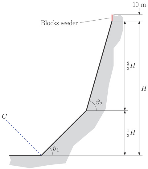
Figure 1.
Sketch of the synthetic double slope profile adopted for the simulations.
The leading idea is that the topography is the parameter that mostly affects the results [42,48,49,50]. This is why, aiming at representing all the most frequent rockfall hazardous situations, the simulations were performed varying only the slope profile, keeping constant the material parameters of both slope and rock blocks, and the model settings. A linear profile, i.e., without any topographic roughness, representing the worst scenario in terms of runout, was considered. The slope angles and of the lower and the upper sections of the profile, respectively, were varied, one by one, between 45 and 90, with an interval of 15, in order to consider typical rockfall prone configurations. A vertical line seeder above the upper section was used to specify a set of source locations for all the simulated rock falls. The source locations were generated with a uniform distribution along the length of the seeder, equal to 10 m. The initial velocity of the falling rocks was set as a deterministic quantity equal to 1 m/s in the vertical downward direction. The assumption of an initial velocity is assumed as precautionary, to consider possible different triggering situations, i.e., earthquake-triggered rockfall, or a complex phenomenon of sliding evolving in free fall of one or more blocks, or detachment due to the impact of blocks from upslope. Normal distributions were adopted for the normal () and the tangential () coefficients of restitution, with mean values of 0.35 and 0.85, respectively, and standard deviation of 0.04 both. On the contrary, the friction coefficient was set as a deterministic quantity equal to . All the adopted parameters were chosen to represent a typical rock slope, according to Bar et al. [51], following the suggestion provided by Pfeiffer and Bowen [52] and Hoek and Bray [53] for bedrock or boulders with little soil or vegetation or just for bedrock in case of lumped mass models. As specifically tailored, the adopted coefficients take into account the limitation in the model kinematics evaluation, e.g., the rotational velocity of the impacting block. These assumptions entail the worst case in terms of propagation, i.e., larger runout distance and lower energy absorption during impact. To increase the accuracy of the results, the number of rocks thrown was set equal to 10,000 with a Monte Carlo sampling technique around the distributions of the restitution coefficients. A collector (C) was positioned at the slope toe, assumed as a flat deposit area, normal to , as to take representative and comparable values of height and velocity.
3.2. Alpha
Several surveys were performed for searching the possible range of the parameter . The parameter is an index of the spread of the block sizes distribution in the location of the net fence: the more heterogeneous the deposit, the lower . The nature of the deposit largely depends on the lithology, the degree of fracturing of the rock mass, and the topography, i.e., slope angle and presence of obstacles on the path [54]. All these aspects influence the kinematics and the possible fragmentation of the blocks. Eight test sites located in the in the Northwestern Italian Alps and characterised by different lithology, exposure, and mean altitude of the source zone were investigated, as reported in Table 1. The surveys were performed manually by counting the size of the blocks, according to the procedure reported in [55,56].

Table 1.
Main characteristics of the test sites and correspondent values.
Figure 2 shows the views of the deposit area of test sites No.3 and No.6 as representative of two opposite situations in terms of heterogeneity in block sizes of the deposit. The figure highlights a wide size variability in test site No.3, while test site No.6 is characterised by a deposit quite homogeneous. The value of was determined through the maximum likelihood estimator [58]:
where N is the number of surveyed blocks and is the mass of each block.
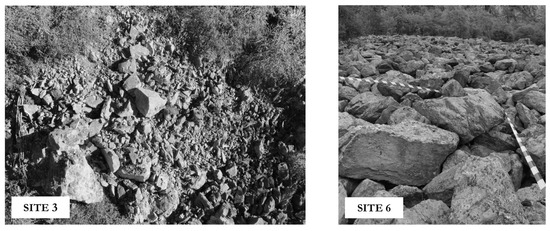
Figure 2.
Views of the test sites No.3 and No.6 for the determination of the parameter . Test site No.3 is characterised by an heterogeneous deposit in terms of block sizes, resulting in . Test site No.6 is characterised by a quite homogeneous deposit in terms of block sizes, resulting in .
3.3. Coefficient of Variation of the Mass
The coefficient of variation is the ratio between the standard deviation and the mean value of a distribution. In the present discussion, this value was considered representative of the spread of the distribution of the block mass at a given return period T, whose relationship follows Equation (1). The parameters of Equation (1), namely and are determined through the observation of past events and by means of a detailed survey of the masses of the blocks where the rockfall net fence is expected to be installed. An uncertainty can be associated to the value of depending on the number of surveyed blocks N. Following Malik [59], the real value of the parameter follows a Chi-square distribution with degrees of freedom [60]. In other words, given the number of surveyed blocks, the maximum likelihood estimator (m.l.e.) provides a “best” value of the parameter, see Equation (15), that, in reality, is distributed as:
where is the variate, i.e., the value of the shape parameter, and is the estimate through the m.l.e. Asymptotic normality is proven for , see [60].
A distribution of masses can be associated to each return period, determined from and Equation (1). The left plot in Figure 3a shows, in black, the distribution of the masses obtained with the procedure previously described for a return period equal to years (, events/yr, , kg). The red curve is the normal distribution that best fits the obtained values. A good agreement between the real distribution of the masses at a given return period and a normal distribution is proven for other return periods, as shown in Figure 3b. This similarity is the hypothesis at the base of the proposed methodology for computing the coefficient of variation of the mass at a given return period. Furthermore, assuming a normal distribution centred in the mean value, instead of a right-skewed Chi-squared distribution, overestimating the impacting block mass, is considered by the authors as precautionary.
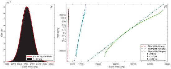
Figure 3.
In (a): distribution of the volume at 20 years return period and normal distribution fit. In (b): normal probability plot with the distributions of the volumes corresponding to three return periods (20 years, 100 years and 500 years). The simulations were performed with , events/yr, , kg. Normally distributed data are identified with a straight line in the probability plot.
To this purpose, (i) the cumulative distribution of the masses was determined, as shown in Figure 4. (ii) Two percentiles were identified, namely 15.87th and 84.13th, which represent the bounds of the mean ± one standard deviation of an equivalent normal distribution. (iii) The masses corresponding to those percentiles are identified, say and . (iv) The standard deviation of the equivalent normal distribution was computed as:
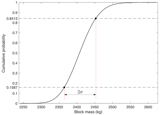
Figure 4.
Cumulative probability distribution of the masses at years (, events/yr, , m). The dots mark the masses corresponding to percentiles 15.87 and 84.13. The difference between the corresponding masses is twice the standard deviation of the equivalent normal distribution.
(v) Supposing that the mean value of the equivalent normal distribution is the mass computed through Equation (1), was computed as
4. Results and Discussion
In this section, the results of the performed analyses are shown and the identified range of parameters is discussed. At the end, the obtained results are adopted to evaluate a range of values associated to different failure probabilities.
4.1. Height and Velocity
Figure 5a,b plot the empirical cumulative distribution of the values of the passing heights and the velocities normalised to the 95th percentile of each parameter. In analogy with what highlighted in Section 3, the results, in terms of both velocity and height, display a huge variety of probability distributions shapes, generally far from a normal one. A large sort of trends is displayed. As a limit situation, in the case in which no rebound occurs (the parabolic solving equation relates to deterministic parameters, only), the cumulative probability density functions of both height and velocity tend to a step curve at or (a Dirac- distribution), respectively.
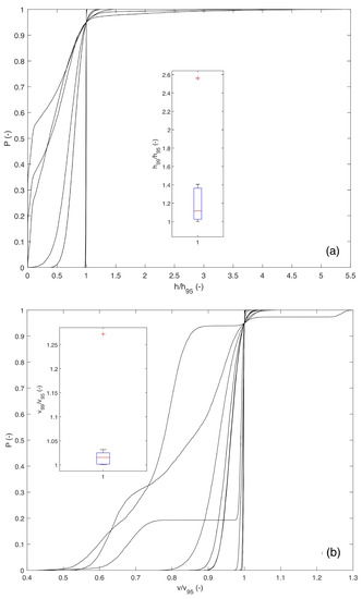
Figure 5.
(a) Cumulative probability distribution function of and the boxplot of , (b) Cumulative probability distribution function of and the boxplot of .
Furthermore, to deeply investigate the statistics of and , Figure 5a,b display the boxplot of both variables. These representations graphically reveal the variation in samples of the statistical populations neglecting their distributions, highlighting the degree of dispersion, the skewness in the data, and showing the outliers. The central red mark indicates the mean, and the bottom and the top edges indicate the 25th () and 75th () percentiles, respectively. The top of the upper whisker is located at . Larger values are considered as outliers (red cross). A different trend can be observed between the considered variables: the height displays right-skewed boxplots, i.e., a positive skew, while the velocity boxplot a slightly left-skewed, i.e., a negative skew. This aspect highlights that both and cannot be related to normal distributions. Each boxplot exhibits an outlier: 2.5 for and 1.27 for . Ignoring the outliers, the 75th percentile of and , are 1.364 and 1.025, respectively. The upper whiskers are located at 1.870 and 1.06 for and , respectively. Considering all the conservative assumption made in modelling the synthetic profiles, the Authors suggest to consider the upper quartile (75th percentile) of each set of ratios as a conservative reference value of and .
4.2. Alpha
Table 1 reports the values of the parameter for each test site. The results span from about 0.7 to 1.6, revealing a great site specificity of this parameter. Nevertheless, comparing the results with those found in [61,62,63], this range encloses the great majority of the cases. Figure 6 plots the complementary cumulative distributions of block volumes related to the eight study cases (left) and the best fitting power law (right).
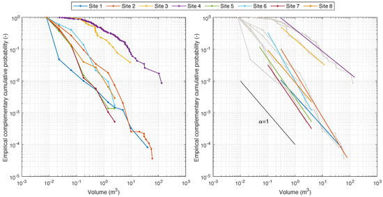
Figure 6.
Empirical complementary cumulative distributions of the surveyed block volumes and the best fitting power laws.
4.3. Coefficient of Variation of the Mass
The procedure proposed in Section 3.3 was applied to define the value of for different T, , and N. Besides, since the coefficient of variation is a ratio, it can be proved that it does not depend on . With reference to the case reported in Figure 4, it results that kg and kg, from which it results kg. Substituting into Equation (1), one gets kg. Thus, the coefficient of variation of the mass is:
The same procedure was repeated for various values of T, , and N. Table 2 reports the values of corresponding to different combinations of the aforementioned parameters. It is shown that the variability of is large and the coefficient is affected by all the four parameters. By interpolation, an approximate expression for was found:
Table 2.
Values of (Coefficient of variation of the mass) for various T, , and N.
5. Towards a Range of Gamma Values
The values of the equivalent partial safety factors are affected by the ratios and , which are related to the slope and rockfall propagation, the parameter , which is related to the impacting block mass distribution, and the coefficient of variation of the mass , which directly depends on the number of surveyed blocks.
The range of such parameters was investigated in the previous section (Section 4). The upper quartiles of the obtained distributions of and , i.e., 1.364 and 1.025, respectively, were considered as representative of the great majority of the propagation kinematics variability. The analysed block mass distributions lead to assume that spans between 0.7 and 1.6. A variable computed according to Equation (20), given the number of surveyed blocks N and , was implemented in the reliability calculations, in particular in computing the failure probability .
Within the above mentioned ranges, the partial safety factors corresponding to various failure probabilities were computed accounting for , i.e., a failure probability equally distributed between a failure related with the excessive height and a failure related to excessive kinetic energy. In the present comparative study, extends from per year to per year. The lower probability corresponds to the annual reliability index (4.7) adopted for civil ordinary structures with a consequence class CC2, according to [30]. To calculate an annual failure probability, was set equal to 1 year.
The simulations were performed considering a mean frequency of events in the range 0.1 and 1 events per year, while the number of surveyed blocks N spans between 200 and 1000. It is assumed that a number of surveyed blocks smaller than 200 does not constitute a statistically representative sample, while larger than 1000 is difficult to achieve. The threshold mass was set to kg. Although the common definition of threshold mass, i.e., the minimum value of the fallen block mass that has always been observed and recorded in the location in which the net fence is expected to be installed [60], this quantity can also be associated to the minimum mass of the impacting block which can be relevant for the design. Two different reference block masses were adopted to compute , i.e., the expected mean masses at a return period of and years, respectively.
Referring to the failure due to excessive kinetic energy, Figure 7 and Figure 8 depict the value of obtained through Equation (14). The values of and are reported in the Appendix A. It clearly emerges that the value of increases as soon as a more safe condition is considered, i.e., the annual failure probability decreases. The heterogeneity of the size of the blocks that can impact the barrier largely affects the value of the coefficients. For in the range 0.7 to 1.0, large values of are observed. This is due to heterogeneity of the impacting blocks sizes resulting in stricter conditions in evaluating the failure probability. On the contrary, a less abrupt, but similar, trend is shown for in the range 1.0 to 1.6. The trend is marginal for years. For a given failure probability, the larger the the smaller the . The influence of the average rockfall frequency is highlighted and it is similar to the effect of the number of surveyed blocks N. The increase of the safety coefficient when the database of a surveyed blocks has low cardinality (i.e., reduced number) can be attributed to the inverse proportionality between N and the coefficient of variation of the mass, . Thus, increasing N, reduces. Similar trends can be observed on both and . The effects of N and are more emphasised on the values of the coefficient of the mass rather than of the velocity. As already mentioned, such trend is a consequence of the influence of N and on . This variation presupposes that a unique value of each partial safety factor cannot be identified, but the problem is strictly site dependent.
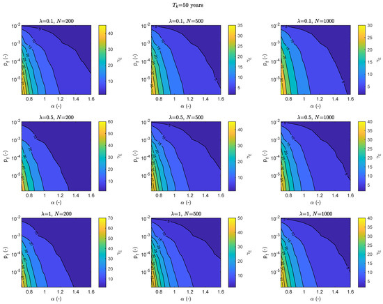
Figure 7.
Partial safety factor related to the energy, , for variable failure probabilities considering a reference block mass having a return period years.
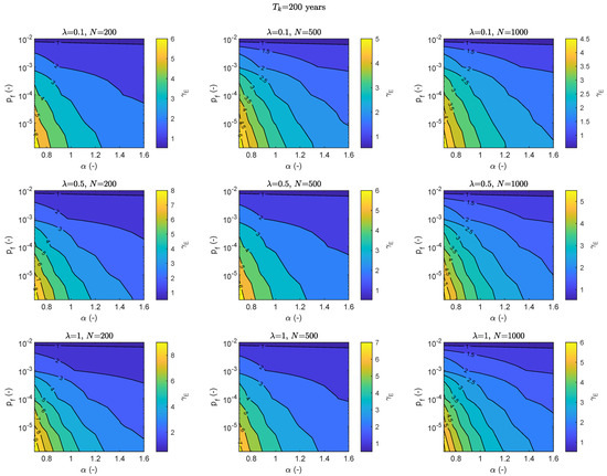
Figure 8.
Partial safety factor related to the energy, , for variable failure probabilities considering a reference block mass having a return period years.
Comparing the results obtained with different return periods through which the characteristic mass is defined, it clearly emerges that higher partial safety factors are obtained for years. A rough comparison between the associated to years and the ones related to years highlights that the latter is more or less 5 or 6 times smaller than the former. The higher rate of decrease is observed for smaller and . The same trend emerges for , while halves its value at years, almost independently from and .
Focusing on the value, in the case of years, the plots show values of , , and, consequently of , larger if compared to those proposed by the Italian and the Austrian national standards. On the contrary, for years, equal to 0.01, the correspondent coefficient is close to one, independently from , N, and .
It is worth mentioning that the suggested values of the above mentioned national standards do not explicitly refer to a failure probability, while they account for a specific time period in which the net fence has to be considered safe, i.e., service life time equal to 25 years [19]. On the contrary, the suggested approach requires to define an annual failure probability not to be exceeded. Furthermore, the standards do not provide any suggestion related to the reference period for the characteristic mass (), computed as a conservative value in the UNI 11211-4 [31] or as a percentile of the cumulative block size distribution in ONR 24810 [32], independently from the occurrence frequency. It reveals that increasing the return period for the characteristic mass the coefficients , , and, consequently, decrease.
Referring to the failure due to excessive height, Figure 9 depicts the values of obtained through Equation (11) as a function of the failure probability . Accounting for the uncertainty on the height of the trajectory of the impacting block, the value of is independent from , as, for the present approach, the tolerance t was assumed as a separate variable, with a Dirac- distribution. The obtained range spans from 1.50 to 2.73, increasing .
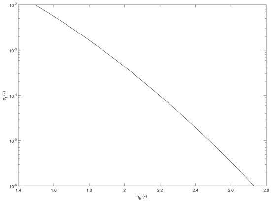
Figure 9.
Partial safety coefficients , as function of the failure probability .
From all these results, it emerges that a unique value of each partial safety factor cannot be identified. Nevertheless, as a first approximation, to partially avoid some uncertainties, the use of a block mass referred to a return period of almost 200 years can be suggested, as well as a minimum number of surveyed blocks N of about 500.
6. Conclusions
A novel time-dependent reliability approach was introduced for the design of rockfall net fences [36]. This method takes into account the variability in time of the the potential impacting mass, as well as the uncertainties related to the size and the kinematics of the impacting block. These parameters were treated as statistical quantities to which a frequency distribution was associated. This design approach was compared to the current practice based on partial safety factors applied to the characteristic values of the impacting block mass, velocity, and height. In De Biagi et al. [36], four variables related to the impacting block were identified as the most influencing parameters, i.e., the ratios and , , and the parameter . Different types of analyses were performed in order to evaluate the possible ranges of the above mentioned parameters representative of the great majority of situations that can be observed in a real rockfall prone area. Rockfall trajectory analyses on synthetic profiles were conducted to investigate and , while onsite surveys served to evaluate the parameter. The coefficient of variation of the mass was investigated assuming a normal distribution of the mass at a given return period. The range of was studied as a function of the number of surveyed blocks N in the area on which the net fence has to be installed, the frequency of the events , and , resulting in an approximate expression, Equation (20).
The obtained results were adopted to evaluate the correspondent values for different failure probabilities. The Authors suggest to adopt and , i.e., the 75th percentile of their distributions, while a range spanning from 0.7 to 1.6 was considered for . The calculations have been performed for annual failure probability from to .
It emerges that the partial safety factor spans from 1.50 to 2.73 according to the failure probability, while, stringently depends on , N, , and on the return period on which the mass is evaluated. Decreasing from 1.0 to 0.7 the rate of change of increases significantly. For a given failure probability, the larger the , the smaller the . A less abrupt, but similar, trend is shown for in the range 1.0 to 1.6. The trend is marginal for years. It can be observed that for greater than 1.1, in case of years, the influence of the failure probability is quite negligible. The influence of is present and it is similar to the effect of the number of surveyed blocks N: the lower the and the higher the N, the lower the . Comparing the results obtained for different return periods , higher partial safety factors are obtained for years: the associated to years are more or less 5 or 6 times higher than the ones related to years. At years, the plot shows values of , , and, consequently of , very high compared to those proposed by the Italian and the Austrian national standards, which do not account for an annual failure probability or for another target value.
The obtained results highlights that the design value for the height of the block can be several times the characteristic value. The same can be observed for the energy in case of short reference return period , and for low value of . This is justified with the fact that the value of the mass changes with the return period.In addition, the number of surveyed blocks N affects the uncertainties related to the characteristic mass and, consequently, the values.
All these considerations result in the fact that, for a given failure probability, quantifying a set of partial safety factors valid for different sites is not possible since they are strictly site dependent. On the contrary, if a set of partial safety factors is assigned to different sites, an intrinsic variability in the failure probability is accepted. As a first suggestion, to partially avoid some uncertainties, the use of a block mass referred to a return period of almost 200 years can be suggested, as well as a surveyed block number N of about 500. Referring to the ratios between velocities and heights, namely and , the Authors suggest to adopt the values herein proposed, which are representative of the 75% of the simulated synthetic profiles. The provided results should be accurately used, accordingly with the required degree of safety. Further developments should be done in order to consider the influence of the mass in the evaluation of the design height, i.e., introducing the block size in the applied tolerance value. Additional scenarios for the trajectory analyses related to different slope profile or input parameters, e.g., restitution coefficients, would be analysed in future researches.
Author Contributions
Conceptualisation, methodology, formal analysis, investigation, M.M. and V.D.B.; writing—original draft preparation, M.M.; writing—review and editing, all the Authors; supervision, D.P.; funding acquisition, V.D.B. and D.P. All authors have read and agreed to the published version of the manuscript.
Funding
This research has been financed under the framework of the research project, titled “Sviluppo di una metodologia per la valutazione del rischio su differenti tipologie di elementi esposti al pericolo di caduta massi” founded by Valle d’Aosta Autonomous Region, Italy and under the “Finanziamento diffuso” grant provided by Politecnico di Torino.
Conflicts of Interest
The authors declare no conflict of interest.
Appendix A. Partial Safety Coefficients Related to the Mass and the Velocity
The partial safety coefficients related to the mass and the velocity for reference masses with return periods 50 and 200 years are reported in the following figures.

Figure A1.
Partial safety factor related to the mass, , for variable failure probabilities considering a reference block mass having a return period years.
Figure A1.
Partial safety factor related to the mass, , for variable failure probabilities considering a reference block mass having a return period years.


Figure A2.
Partial safety factor related to the mass, , for variable failure probabilities considering a reference block mass having a return period years.
Figure A2.
Partial safety factor related to the mass, , for variable failure probabilities considering a reference block mass having a return period years.


Figure A3.
Partial safety factor related to the velocity, , for variable failure probabilities considering a reference block mass having a return period years.
Figure A3.
Partial safety factor related to the velocity, , for variable failure probabilities considering a reference block mass having a return period years.


Figure A4.
Partial safety factor related to the velocity, , for variable failure probabilities considering a reference block mass having a return period years.
Figure A4.
Partial safety factor related to the velocity, , for variable failure probabilities considering a reference block mass having a return period years.

References
- Corominas, J.; Moya, J. A review of assessing landslide frequency for hazard zoning purposes. Eng. Geol. 2008, 102, 193–213. [Google Scholar] [CrossRef]
- Jaboyedoff, M.; Dudt, J.P.; Labiouse, V. An attempt to refine rockfall hazard zoning based on the kinetic energy, frequency and fragmentation degree. Nat. Hazards Earth Syst. Sci. 2005, 5, 621–632. [Google Scholar] [CrossRef]
- Ferrari, F.; Giacomini, A.; Thoeni, K. Qualitative rockfall hazard assessment: A comprehensive review of current practices. Rock Mech. Rock Eng. 2016, 49, 2865–2922. [Google Scholar] [CrossRef]
- Scavia, C.; Barbero, M.; Castelli, M.; Marchelli, M.; Peila, D.; Torsello, G.; Vallero, G. Evaluating rockfall risk: Some critical aspects. Geosciences 2020, 10, 98. [Google Scholar] [CrossRef]
- Mignelli, C.; Russo, S.L.; Peila, D. ROckfall risk MAnagement assessment: The RO. MA. approach. Nat. Hazards 2012, 62, 1109–1123. [Google Scholar] [CrossRef]
- Mineo, S.; Pappalardo, G.; D’urso, A.; Calcaterra, D. Event tree analysis for rockfall risk assessment along a strategic mountainous transportation route. Environ. Earth Sci. 2017, 76, 620. [Google Scholar] [CrossRef]
- Mineo, S. Comparing rockfall hazard and risk assessment procedures along roads for different planning purposes. J. Mt. Sci. 2020, 17, 653–669. [Google Scholar] [CrossRef]
- Macciotta, R.; Martin, C.D.; Morgenstern, N.R.; Cruden, D.M. Quantitative risk assessment of slope hazards along a section of railway in the Canadian Cordillera—A methodology considering the uncertainty in the results. Landslides 2016, 13, 115–127. [Google Scholar] [CrossRef]
- Lopez-Saez, J.; Corona, C.; Eckert, N.; Stoffel, M.; Bourrier, F.; Berger, F. Impacts of land-use and land-cover changes on rockfall propagation: Insights from the Grenoble conurbation. Sci. Total Environ. 2016, 547, 345–355. [Google Scholar] [CrossRef]
- Volkwein, A.; Schellenberg, K.; Labiouse, V.; Agliardi, F.; Berger, F.; Bourrier, F.; Dorren, L.K.; Gerber, W.; Jaboyedoff, M. Rockfall characterisation and structural protection—A review. Nat. Hazards Earth Syst. Sci. 2011, 11, 2617–2651. [Google Scholar] [CrossRef]
- Yu, Z.; Qiao, Y.; Zhao, L.; Xu, H.; Zhao, S.; Liu, Y. A simple analytical method for evaluation of flexible rockfall barrier. Part 1: Working mechanism and analytical solution. Adv. Steel Constr. 2018, 14, 115–141. [Google Scholar]
- Chanut, M.A.; Dubois, L.; Nicot, F. Dynamic behavior of rock fall protection net fences: A parametric study. In Engineering Geology for Society and Territory; Springer: Berlin, Germany, 2015; Volume 2, pp. 1863–1867. [Google Scholar]
- Castanon-Jano, L.; Blanco-Fernandez, E.; Castro-Fresno, D.; Ballester-Muñoz, F. Energy dissipating devices in falling rock protection barriers. Rock Mech. Rock Eng. 2017, 50, 603–619. [Google Scholar] [CrossRef]
- Xu, H.; Gentilini, C.; Yu, Z.; Qi, X.; Zhao, S. An energy allocation based design approach for flexible rockfall protection barriers. Eng. Struct. 2018, 173, 831–852. [Google Scholar] [CrossRef]
- Marchelli, M.; De Biagi, V.; Peila, D. A quick-assessment procedure to evaluate the degree of conservation of rockfall drapery meshes. Frat. Ed Integrità Strutt. 2019, 13, 437–450. [Google Scholar] [CrossRef]
- Peila, D.; Ronco, C. Design of rockfall net fences and the new ETAG 027 European guideline. Nat. Hazards Earth Syst. Sci. 2009, 9, 1291–1298. [Google Scholar] [CrossRef]
- Volkwein, A.; Gerber, W.; Klette, J.; Spescha, G. Review of approval of flexible rockfall protection systems according to ETAG 027. Geosciences 2019, 9, 49. [Google Scholar] [CrossRef]
- Guideline for European Technical Approval of Falling Rock Protection Kits; ETAG 027; European Organisation for Technical Approvals (EOTA): Brusseles, Belgium, 2008.
- Falling Rock Protection Kits; EAD 340059-00-0106; European Organisation for Technical Approvals (EOTA): Brusseles, Belgium, 2018.
- Bourrier, F.; Baroth, J.; Lambert, S. Accounting for the variability of rock detachment conditions in designing rockfall protection structures. Nat. Hazards 2016, 81, 365–385. [Google Scholar] [CrossRef]
- Toe, D.; Mentani, A.; Govoni, L.; Bourrier, F.; Gottardi, G.; Lambert, S. Introducing meta-models for a more efficient hazard mitigation strategy with rockfall protection barriers. Rock Mech. Rock Eng. 2018, 51, 1097–1109. [Google Scholar] [CrossRef]
- Bertrand, D.; Trad, A.; Limam, A.; Silvani, C. Full-scale dynamic analysis of an innovative rockfall fence under impact using the discrete element method: From the local scale to the structure scale. Rock Mech. Rock Eng. 2012, 45, 885–900. [Google Scholar] [CrossRef]
- Cazzani, A.; Mongiovì, L.; Frenez, T. Dynamic finite element analysis of interceptive devices for falling rocks. Int. J. Rock Mech. Min. Sci. 2002, 39, 303–321. [Google Scholar] [CrossRef]
- Dugelas, L.; Coulibaly, J.; Bourrier, F.; Olmedo, I.; Chanut, M.; Lambert, S.; Nicot, F.; Dugelas, L.; Coulibaly, J.; Bourrier, F.; et al. Comparison of Two DEM Modeling of Flexible Rockfall Fences under Dynamic Impact. Available online: www.hal.archives-ouvertes.fr/hal-01997731 (accessed on 22 July 2020).
- Gentilini, C.; Gottardi, G.; Govoni, L.; Mentani, A.; Ubertini, F. Design of falling rock protection barriers using numerical models. Eng. Struct. 2013, 50, 96–106. [Google Scholar] [CrossRef]
- Qi, X.; Yu, Z.X.; Zhao, L.; Xu, H.; Zhao, S.C. A new numerical modelling approach for flexible rockfall protection barriers based on failure modes. Adv. Steel Constr. 2018, 14, 479–495. [Google Scholar] [CrossRef]
- Govoni, L.; de Miranda, S.; Gentilini, C.; Gottardi, G.; Ubertini, F. Modelling of falling rock protection barriers. Int. J. Phys. Model. Geotech. 2011, 11, 126–137. [Google Scholar] [CrossRef]
- Koo, R.C.; Kwan, J.S.; Lam, C.; Ng, C.W.; Yiu, J.; Choi, C.E.; Ng, A.K.; Ho, K.K.; Pun, W.K. Dynamic response of flexible rockfall barriers under different loading geometries. Landslides 2017, 14, 905–916. [Google Scholar] [CrossRef]
- Toe, D.; Mentani, A.; Gottardi, G.; Bourrier, F. A Novel Approach to Assess the Ability of a Protection Barrier to Mitigate Rockfall Hazard. In Proceedings of the Symposium Proceedings of the INTERPRAENENT 2018 in the Pacific Rim, Toyama, Japan, 1–4 October 2018; pp. 249–257. [Google Scholar]
- Eurocode 0—Basis of Structural Design; EN 1990:2002; European Committee for Standardization (CEN): Brusseles, Belgium, 2002.
- Opere di Difesa Dalla Caduta Massi—Parte 4: Progetto Definitivo ed Esecutivo; UNI 11211-4; Ente Italiano di Unificazione (UNI): Roma, Italy, 2018.
- Technical Protection Against Rockfall—Terms and Definitions, Effects of Actions, Design, Monitoring and Maintenance; ONR 24810; ONR (Austrian Standards International): Wien, Austria, 2017.
- Agliardi, F.; Crosta, G.B. High resolution three-dimensional numerical modelling of rockfalls. Int. J. Rock Mech. Min. Sci. 2003, 40, 455–471. [Google Scholar] [CrossRef]
- Dorren, L.K. Rockyfor3D (v5. 2) revealed—Transparent description of the complete 3D rockfall model. EcorisQ Paper. 2015. Available online: www.ecorisq.org (accessed on 22 July 2020).
- Leine, R.; Schweizer, A.; Christen, M.; Glover, J.; Bartelt, P.; Gerber, W. Simulation of rockfall trajectories with consideration of rock shape. Multibody Syst. Dyn. 2014, 32, 241–271. [Google Scholar] [CrossRef]
- De Biagi, V.; Marchelli, M.; Peila, D. Reliability analysis and partial safety factors approach for rockfall protection structures. Eng. Struct. 2020, 213, 110553. [Google Scholar] [CrossRef]
- Melchers, R.E.; Beck, A.T. Structural Reliability Analysis and Prediction; John Wiley & Sons: Hoboken, NJ, USA, 2018. [Google Scholar]
- De Biagi, V.; Botto, A.; Napoli, M.; Dimasi, C.; Laio, F.; Peila, D.; Barbero, M. Calcolo del tempo di ritorno dei crolli in roccia in funzione della volumetria. GEAM Geoing. Ambient. Mineraria 2016, 53, 39–48. [Google Scholar]
- De Biagi, V.; Napoli, M.L.; Barbero, M.; Peila, D. Estimation of the return period of rockfall blocks according to their size. Nat. Hazards Earth Syst. Sci. 2017, 17, 103–113. [Google Scholar] [CrossRef]
- De Biagi, V.; Napoli, M.L.; Barbero, M. A quantitative approach for the evaluation of rockfall risk on buildings. Nat. Hazards 2017, 88, 1059–1086. [Google Scholar] [CrossRef]
- Glover, J.; Schweizer, A.; Christen, M.; Gerber, W.; Leine, R.; Bartelt, P. Numerical investigation of the influence of rock shape on rockfall trajectory. EGU Gen. Assem. Conf. Abstr. 2012, 14, 11022. [Google Scholar]
- Wang, I.T.; Lee, C.Y. Influence of slope shape and surface roughness on the moving paths of a single rockfall. World Acad. Sci. Eng. Technol. 2010, 65, 1021–1027. [Google Scholar]
- Fischer, L.; Purves, R.S.; Huggel, C.; Noetzli, J.; Haeberli, W. On the influence of topographic, geological and cryospheric factors on rock avalanches and rockfalls in high-mountain areas. Nat. Hazards Earth Syst. Sci. 2012, 12, 241–254. [Google Scholar] [CrossRef]
- Nishimura, T.; Kiyama, H.; Fukuda, T. Parametric three-dimensional simulations of dispersion of rockfall trajectories. In The 42nd US Rock Mechanics Symposium (USRMS); American Rock Mechanics Association: Alexandria, VA, USA, 2008. [Google Scholar]
- Keylock, C.; Domaas, U. Evaluation of topographic models of rockfall travel distance for use in hazard applications. Arct. Antarct. Alp. Res. 1999, 31, 312–320. [Google Scholar] [CrossRef]
- Musakale, F.B. Influence of Bench Geometries on Rockfall Behaviour in Open Pit Mines. Master’s Thesis, University of Witwatersrand, Johannesburg, South Africa, 2005. [Google Scholar]
- RocScience Inc. RocFall, User’s Guide; RocScience Inc.: Toronto, ON, Canada, 1998–2002. [Google Scholar]
- Ritchie, A.M. Evaluation of Rockfall and Its Control; Technical Report 17; Highway Research Record; Transportation Research Board: Washington, DC, USA, 1963. [Google Scholar]
- Pierson, L.A.; Davis, S.A.; Pfeiffer, T.J. The Nature of Rockfall as the Basis for a New Fallout Area Design Criteria for 0.25: 1 Slopes; Technical Report; Department of Transportation, Geotechnical Services Unit: Portland, OR, USA, 1994.
- Volta, F. Il Ruolo Delle Barriere Paramassi Nella Mitigazione del Rischio da Frana Nella Provincia Autonoma di Bolzano. Master’s Thesis, Università di Bologna, Bologna, Italy, 2011. [Google Scholar]
- Bar, N.; Nicoll, S.; Pothitos, F. Rock fall trajectory field testing, model simulations and considerations for steep slope design in hard rock. In Proceedings of the First Asia Pacific Slope Stability in Mining Conference, Brisbane, Australia, 6–8 September 2016; pp. 457–466. [Google Scholar]
- Pfeiffer, T.J.; Bowen, T. Computer simulation of rockfalls. Bull. Assoc. Eng. Geol. 1989, 26, 135–146. [Google Scholar] [CrossRef]
- Hoek, E.; Bray, J.D. Rock Slope Engineering; CRC Press: Boca Raton, FL, USA, 1981. [Google Scholar]
- Umili, G.; Bonetto, S.M.; Mosca, P.; Vagnon, F.; Ferrero, A.M. In Situ Block Size Distribution Aimed at the Choice of the Design Block for Rockfall Barriers Design: A Case Study along Gardesana Road. Geosciences 2020, 10, 223. [Google Scholar] [CrossRef]
- Marchelli, M.; De Biagi, V. Optimization methods for the evaluation of the parameters of a rockfall fractal fragmentation model. Landslides 2019, 16, 1385–1396. [Google Scholar] [CrossRef]
- Marchelli, M.; De Biagi, V.; Grange, H.; Peila, D. Applicazione del modello di frammentazione frattale ad un caso reale di caduta massi. Problematiche inerenti la scelta dei parametri di modello. Geoing. Ambient. Mineraria 2019, 157, 22–32. [Google Scholar]
- Barbero, M.; Castelli, M.; Cavagnino, G.; De Biagi, V.; Scavia, C.; Vallero, G. Application of a Statistical Approach for the Assessment of Design Block in Rockfall: A Case Study in Sesia Valley (Northern Italy). In National Conference of the Researchers of Geotechnical Engineering; Springer: Berlin, Germany, 2019; pp. 621–629. [Google Scholar]
- Arnold, B.C. Pareto distributions. Monographs on Statistics and Applied Probability (140); CRC Press: Boca Raton, FL, USA, 2015; pp. 1–408. [Google Scholar]
- Malik, H.J. Estimation of the parameters of the Pareto distribution. Metrika 1970, 15, 126–132. [Google Scholar] [CrossRef]
- De Biagi, V. Brief communication: Accuracy of the fallen blocks volume-frequency law. Nat. Hazards Earth Syst. Sci. 2017, 17, 1487–1492. [Google Scholar] [CrossRef]
- Ruiz-Carulla, R.; Corominas, J.; Mavrouli, O. A methodology to obtain the block size distribution of fragmental rockfall deposits. Landslides 2015, 12, 815–825. [Google Scholar] [CrossRef]
- Ruiz-Carulla, R.; Corominas, J.; Mavrouli, O. Comparison of block size distribution in rockfalls. In Landslides and Engineered Slopes. Experience, Theory and Practice; CRC Press: Boca Raton, FL, USA, 2016; pp. 1767–1774. [Google Scholar]
- Crosta, G.B.; Frattini, P.; Fusi, N. Fragmentation in the Val Pola rock avalanche, Italian alps. J. Geophys. Res. Earth Surf. 2007, 112. [Google Scholar] [CrossRef]


© 2020 by the authors. Licensee MDPI, Basel, Switzerland. This article is an open access article distributed under the terms and conditions of the Creative Commons Attribution (CC BY) license (http://creativecommons.org/licenses/by/4.0/).