Article

Prospecting and Evaluation of Underground Massive Ice by Ground-Penetrating Radar

Chersky Mining Institute of the North, Siberian Branch, RAS, Yakutsk 677980, Russia
*
Author to whom correspondence should be addressed.
Geosciences 2020, 10(7), 274; https://doi.org/10.3390/geosciences10070274
Submission received: 3 June 2020 / Revised: 1 July 2020 / Accepted: 13 July 2020 / Published: 16 July 2020
(This article belongs to the Special Issue Modern Surveying and Geophysical Methods for Soil and Rock)

Abstract

:
Data from geocryological studies of soil and rock massifs in permafrost zone are very important as a basis for predicting possible negative consequences associated with climate change. A promising technique for studying geocryological structures (various types of underground ice) is the ground-penetrating radar (GPR) method. This paper presents the applications of the GPR method to prospect and evaluate massive ice in a frozen rock mass. To study the features of GPR signals received during sounding of underground ice, a model of a single GPR trace for the structure “frozen rock-ice-frozen rock” was developed. As a result, regularities were established in the kinematic and dynamic characteristics of GPR signals at the upper and lower boundaries of massive ice, depending on its geometric parameters. The established features were confirmed by the results of computer and physical simulation of GPR measurements of a frozen rock mass model. The main result of the study was to obtain a set of criteria for identifying massive ice according to GPR measurements. The developed criteria will allow the use of GPR for a detailed study of the structure of permafrost rocks to prevent the development of dangerous cryogenic processes in undisturbed and urban areas of the Arctic.

1. Introduction

Currently, intensive development of territories located in the permafrost zone is increasing [1]. Under the conditions of climate warming in the Arctic [2], it is necessary to assess the risk of geological hazards, as permafrost thawing affects not only the geomorphology of the Arctic, but also existing ecosystems and infrastructure [3,4,5,6,7]. Safe operation of engineering structures is an important factor for the life and health of citizens. This factor requires constant monitoring and study, in order to predict the possible negative consequences associated with climate warming. As shown by many years of research in the Russian Artic regions, the loss of bearing capacity of soils may be the main danger to the operation of engineering structures [8]. Even the partial destruction of vital engineering structures in winter, can lead to significant human and material losses. When studying the bearing capacity of soils, it is very important to financially support the relevant studies, since it is necessary to reduce costs without losing the quality of information received. In this regard, the urgent problem is the development of methods for the study and monitoring of rock masses and soil of the Arctic, the thawing of which can lead to destruction or deformation of engineering structures.
The review [9] presents the methodological backgrounds of monitoring and modeling the processes of climate change in northern Europe. According to the authors, one of the key properties of rocks and permafrost soils is the presence of ice in them.
The main problem that does not allow reliable assessment of the consequences of soil thawing is the lack of accurate information on the presence of various types of underground ice [10], which are widespread in soils and rocks of the permafrost zone [11,12,13]. The existing permafrost-landscape maps [14] are of large scale, which does not allow informed engineering, technical, and geotechnical decisions to be made [15].
Traditional methods of geocryology used to study frozen rocks require improvement [16], because the data obtained by these methods, as a rule, are point-like, and do not allow full evaluation of the geocryological conditions in sufficiently large areas. Several modern methods of geocryology include methods of geophysics (for example, vertical electric sounding [16]), which can be used to search and determine the parameters of underground ice.
For more than 30 years [17,18,19,20,21,22,23,24,25,26], methods of geophysics have been used to study rocks and soils in the permafrost zone. The review [27] presents the positively proven geophysical methods. Currently, there is positive experience in studying vein ice [28,29,30,31,32,33,34], massive ice [35,36,37], zones of high ice content [17], pingo ice [38,39], and cave ice [40,41].
As shown by many years of geophysical research of underground ice, in some cases it is possible to determine the presence of underground ice using a small number of reference and confirmatory wells [35], while involving a complex of geophysical methods. However, in most cases, the geocryological interpretation of the obtained geophysical data is rather complicated. If the criteria for determining vein ice follow from its genesis and it is easily determined due to its polygonal shape [28], then, for example, massive ice is much more difficult to detect.
To successfully prospect and evaluate massive ice, first of all, it is necessary to choose the appropriate geophysical method. To this end, we reviewed publications, which showed that the paper [37] presents the results of a study comparing the effectiveness of various geophysical methods for studying underground ice. The authors of the article came to the conclusion that for the study of massive ice (less than 50 m thick) located in the permafrost zone it is possible to use the GPR method, which has also been used by other researchers for this purpose [34,37]. The advantages of the GPR method are the efficiency and the cost of measurements when studying the structure of frozen rock massifs [38]. The disadvantages of GPR include the complex processing of signals and the difficulties in determining the physical and mechanical properties of rocks.
Using the GPR, it is quite simple to prospect and estimate the size of underground ice, if you know for certain about its availability from a priori data (drilling data or outcrops inspection). In the absence of reliable and sufficiently complete a priori data, it is very difficult to determine the presence of massive ice from GPR data. On the GPR data (radargram) there is displayed a separate area (georadar-stratigraphic unit [35]), bounded above and below by horizontal serial signals (events), which are obtained as a result of signal reflection from the upper and lower ice boundaries. In order to check ice or an undisturbed rock layer, it is necessary to drill wells each time a similar wave pattern appears on the radargram, which significantly increases the cost of geophysical work.
To reduce the cost of drilling wells, it is necessary to find a way to distinguish between the ice layer from the rock formation according to GPR measurements.
The purpose of this study was to validate and test the criteria for identifying massive ice based on the results of GPR surveys. Permafrost scientists call the term “massive ice” as there are three types of deposit-forming ice (pure, horizontally layered with mineral layers, ice with mineral impurities). In our study, we mean by “massive ice” the ice of the first type, i.e. pure, which is important for choosing the used values of the electrophysical properties.
The proposed criteria are based on knowledge of the characteristics of the propagation process of electromagnetic waves in the geology and the typical values of the electrophysical properties of ice and the surrounding rocks. To develop the criteria, we have undertaken the following:
  • created and analyzed a model of a single GPR trace for frozen rock mass with massive ice;
  • conducted computer and physical simulation of GPR sounding of a frozen rock mass model with the inclusion of massive ice.
When performing step 1, we obtained theoretical values of the parameters of GPR signals which were then compared with the results of computer and physical simulation.

2. Method of Experimental Studies

2.1. GPR Method

Serially produced ground penetrating radars currently use antennas to emit and receive ultra-wideband pulses with a central frequency (fc) of 10 to 2000 MHz, which corresponds to wavelengths in frozen rocks from 12 m to 0.12 m. The principle of GPR operation is based on reflection of electromagnetic waves from the interface of geological environments having different electrophysical properties (dielectric constant ε and electrical conductivity σ). The presence of such surfaces in rock masses is due to the difference not only in the mineral and granulometric composition of rocks, but also in the density, moisture content, cryogenic state, etc.
The GPR data consists of a set of traces (radargrams), which are a set of signals reflected from the interface of geological environments. The signals consist of alternating pulses with positive and negative amplitudes. The signals are visualized in the form of several black (positive values) and white (negative values) stripes, which are called “events," the shape of which repeats the shape of the interface.
Each signal can be characterized by the following parameters:
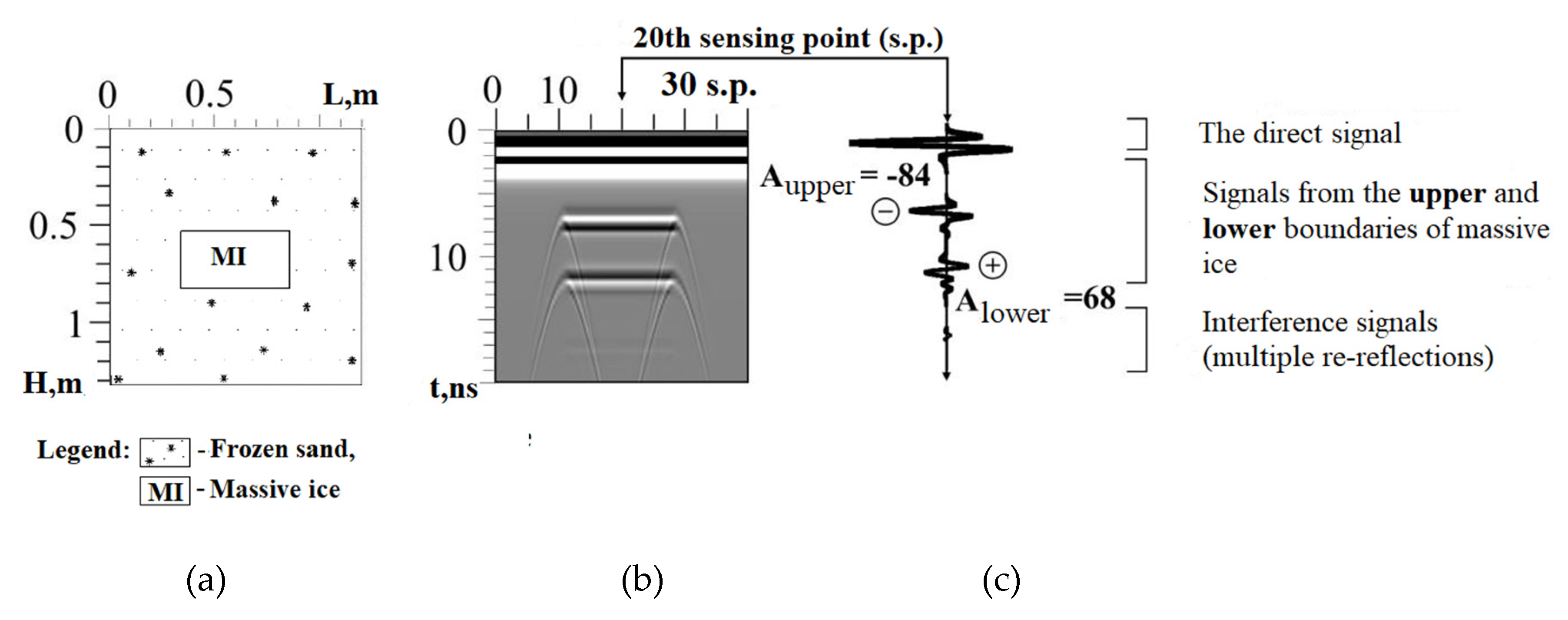
  • amplitude—the magnitude of the maximum pulse (A);
  • phase (with what impulse the signal starts, negative or positive);
  • traveltime (t);
  • center frequency of the Fourier spectrum (fc).

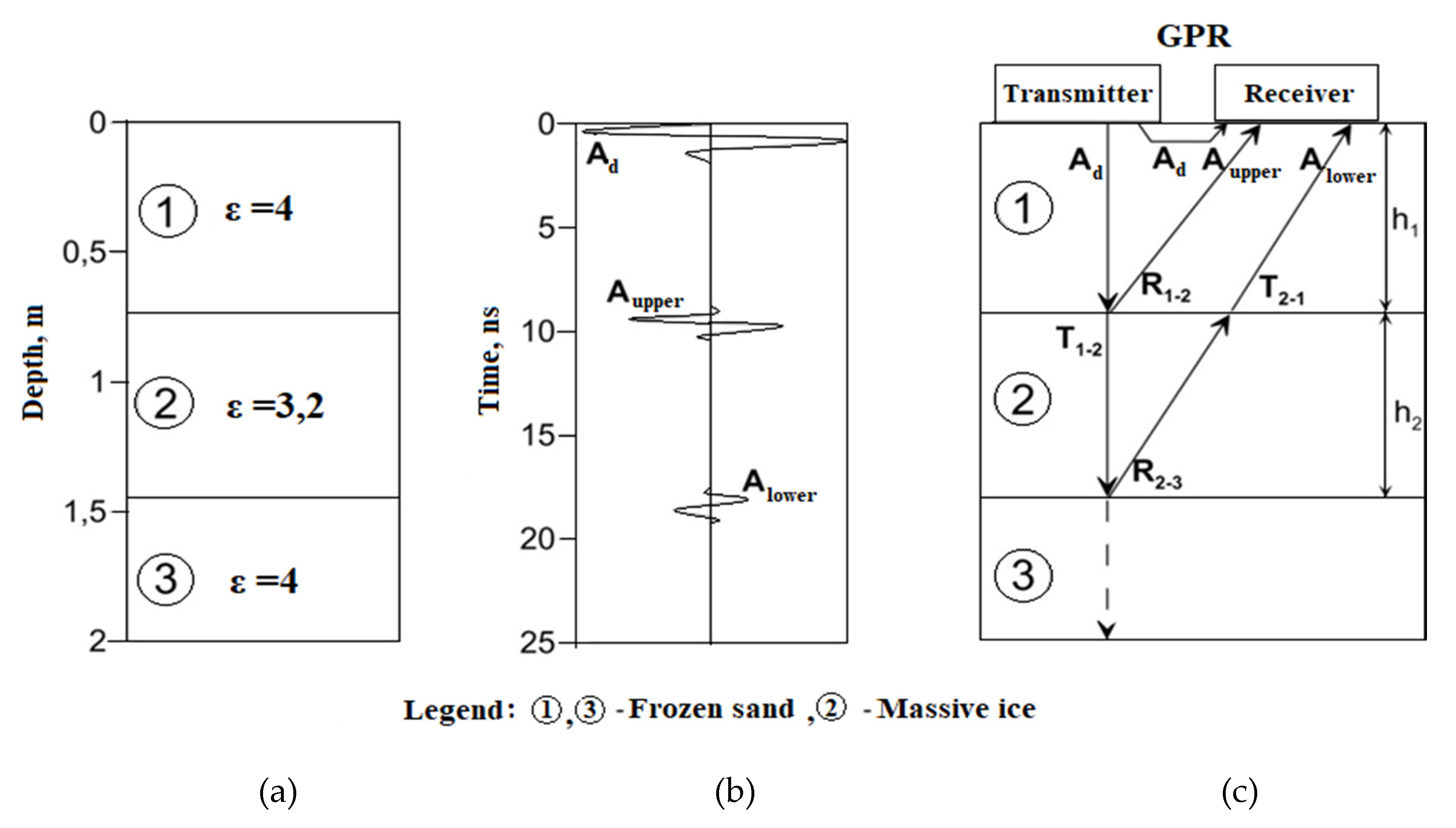
2.2. Theoretical Foundations of Massive Ice Detection by GPR

A GPR model was created to determine the characteristics of the radiophysical parameters of the signals common to massive ice in a frozen rock mass (Figure 1). It consists of the host medium represented by frozen sand with the inclusion of ice with a thickness of h = 0.72 m at a depth of H = 0.72 m. Electrophysical parameters of the model objects are specified as the real part of the complex relative permittivity (ε′), frozen sand-ε′ = 4, ice-ε′ = 3.2 [42]., which determines the propagation velocity of electromagnetic waves (in sand vfs = 0.15 m/ns, in ice vi = 0.168 m/ns). The ε′ values of frozen sand are from 4 to 5 in the conditions of the north of the Asian part of Russia. We chose the value ε′ = 4 for our study, which is without restriction, and all of the following formulas can be recalculated for any value ε′ necessary for the reader.
For this GPR model, a single GPR trace s(t) describing itself as a combination of useful signals p(t) and interference n(t) was developed. The component p(t) consists of the sum of the direct signal AdU(t) and the signals from the upper AupperU(ttupper) and lower AlowerU(ttlower) ice boundaries, where:
U(t) is a function that describes the shape of the GPR signal;
Aupper, Alower—the amplitude values of the signals, depending on the reflection coefficient R at the upper and lower ice boundaries, as well as on the absorption of electromagnetic energy (γ) in frozen sand and ice;
tupper and tlower—traveltime of the signal from the upper and lower ice boundaries, respectively (tupper = 2h1/vfs; tlower = tupper + 2h2/vi).
Assume that the signal amplitude emitted by the GPR is equal to Ad, then according to [39] the amplitude of the wave reflected from the upper ice boundary will be equal to
A upper = A d R 1 - 2 e 2 γ 1 h 1
where R1-2 = 0.055 is the reflection coefficient from the “frozen sand–ice” boundary, γ1 is the propagation constant describing the attenuation of the electromagnetic wave propagating in frozen sand, and h1 is the thickness of frozen sand.
The coefficient R1-2 is calculated by the formula
R 1 - 2 = ε 1 ε 2 ε 1 + ε 2
The amplitude of the wave reflected from the lower ice boundary will be equal to
A lower = A d T 1 - 2 T 2 - 1 R 2 - 3 e 2 γ 1 h 1 e 2 γ 2 h 2
where T1-2, T2-1 are the transmission coefficients at the upper ice boundary (T = 1 − R), h2 is the thickness of the ice. The reflection coefficient on the lower ice boundary is less than zero (R2-3 = −R1-2 = −0.055), which leads to a change in the signal phase.
Based on the foregoing, a model of the GPR trace obtained by sounding of a frozen rock mass containing massive ice can be represented as
s(t) = AdU(t) + 0.055Ade−2 γ1h1U(tt1) + (−0.055)Ade−2(γ1h1+ γ2h2) U(tt2) + n(t)
The value of the amplitude Ad of the sounding signal depends both on the features of the GPR hardware and software and on the electrophysical properties of the rock on which the GPR is installed. It does not allow the use of the Aupper and Alower values in the analysis, processing, and interpretation of the GPR data. However, the ratio of these quantities does not depend on the amplitude of Ad
A l o w e r A u p p e r = A п T 1 2 T 2 1 R 2 3 e 2 γ 1 h 1 e 2 γ 2 h 2   A п R 1 2 e 2 γ 1 h 1 = ( 1 R 1 2 2 ) e 2 γ 2 h 2
For pure ice, the specific attenuation γ2 = 0.3 dB/m, the propagation velocity of the electromagnetic wave V2 = 0.168 m/ns, which allows us to simplify formula (5) based on h2 = t V 2 2
A l o w e r A u p p e r = ( 1 0.055 2 ) e 2 γ 2 t V 2 2 = 0.99 e 2 * 0.3 * 0.008 t = 0.95 t
where ∆t is the double transit time of the electromagnetic wave in the massive ice.
According to the literature [43,44,45,46,47], the specific attenuation in existing ice at frequencies of about 1 GHz is more than 0.3 dB/m; therefore, the ratio of the amplitude values of the signals obtained in the practice of the GPR measurements is less than 0.95∆t.
When interpreting the GPR data, it is more convenient to check whether the electromagnetic ice attenuation value γ2, defined as
20 l g ( A l o w e r A u p p e r ) = 20 l g ( A d T 1 2 T 2 1 R 2 3 e 2 γ 1 h 1 e 2 γ 2 h 2 ) 20 l g ( A d R 1 2 e 2 γ 1 h 1 )
with transmission coefficients:
T 1 2 = 1 + R 1 2
T 2 1 = 1 R 1 2
Transforming Equation (7), taking into account the fact that (1 + R1-2) (1 − R1-2) = 1 − R1-22 and that the media 1 and 3 are the same, then after reducing the similar elements in Equation (7), we get
20 l g e ( A l o w e r A u p p e r ) = 20 l g ( 1 R 1 2 2 ) + 20 l g e 2 γ 2 h 2
From the Equation (8), we find the specific attenuation
20 l g e ( 2 γ 2 h 2 ) = 20 l g ( 1 R 1 2 2 ) 20 l g ( A l o w e r A u p p e r )
20 l g e   ( 2 γ 2 h 2 ) = 20 l g ( 0.99 A u p p e r A l o w e r )
2 γ 2 h 2 = 20 l g ( 0.99 A u p p e r A l o w e r ) 20 l g e
Finally, we get the equation for specific attenuation in decibels
γ 2 = 20 l g ( 0.99 A u p p e r A l o w e r ) 17.3 h 2 = 1 0.16 t l g ( 0.99 A u p p e r A l o w e r )
where h2 is determined by the formula h 2 = t V 2 2 .
In the GPR trace model, the interference n(t) is a multiple and diffracted signal having the same shape as the useful signals. The Fourier spectrum of such interference on average coincides with the Fourier spectrum of a single signal [48] and this incomplete correspondence is displayed in the form of fluctuations of the envelope Fourier spectrum of the entire GPR trace. The shape of the envelope Fourier spectrum of the trace is also affected by the thickness of ice, expressed as the double transit time of the electromagnetic wave Δt, because in this case, the ice acts as a comb rejection filter for the frequencies k/Δt (where k = 0, 1, 2 ...), which leads to a “ripple” shape of the spectrum, even in the absence of various interference.
To confirm the correctness of the developed model of a single GPR trace and the formulas (6) and (12), computer and physical simulation of GPR measurements of frozen rock mass containing massive ice were carried out.

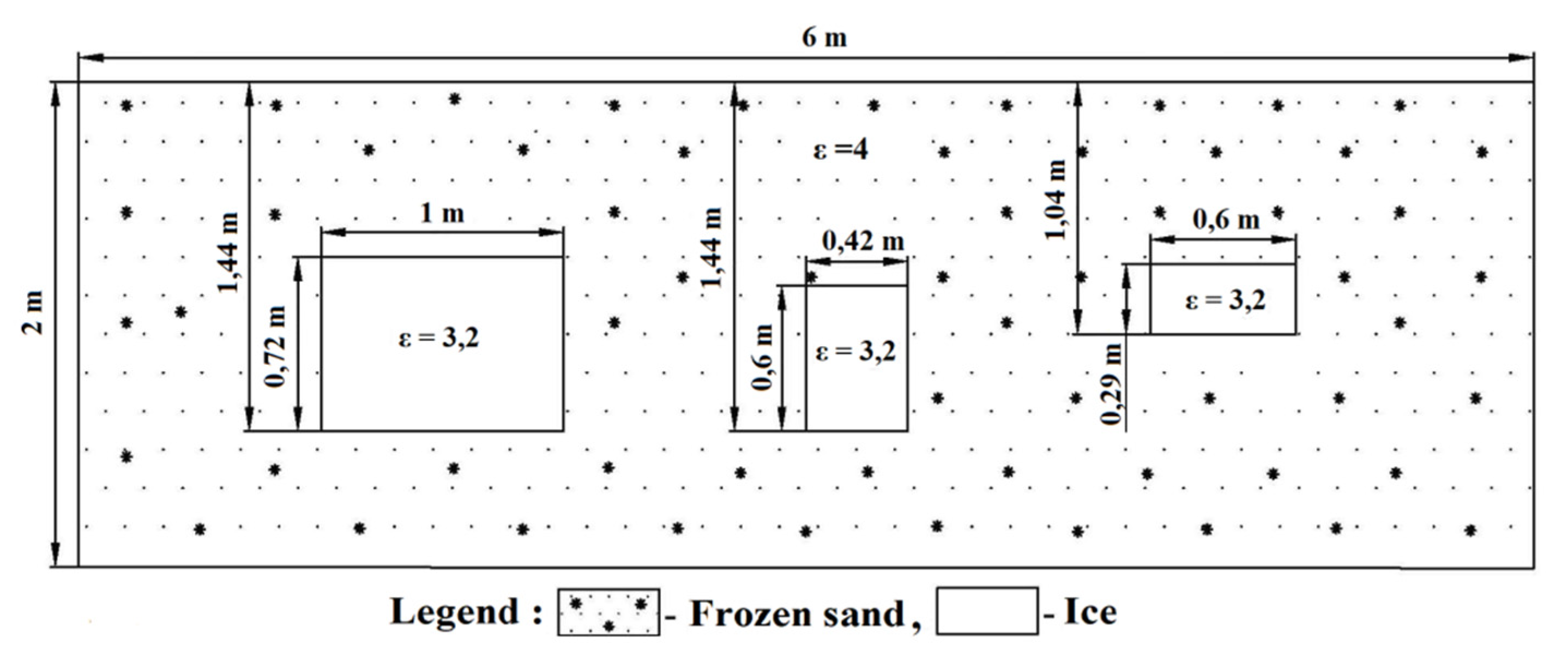
2.3. Computer Simulation of GPR Measurements

To simulate the electromagnetic wave propagation in a geological environment, we used the gprMax software that solves Maxwell’s equations using the finite difference-time domain method (FDTD) [49].
Computer simulation was performed for the GPR with a central frequency of the emitted spectrum fc = 1200 MHz (the maximum depth of the study is 1.5 m with a resolution of 0.05 m), which was chosen based on the size of the frozen rock mass model with massive ice for two models:
  • with one sample of massive ice in a frozen host medium;
  • with three samples of massive ice in a frozen host medium.
The second model is necessary for a visual assessment of the received GPR signals from the ice of different sizes. The GPR model with one ice sample with a thickness h = 0.29 m, length L = 0.5 m, located at a depth of H = 0.5 m in the host medium is represented by frozen sand (1.2 × 1.3m). The electrophysical parameters of the model objects are specified as the real part of the complex relative permittivity (ε′), ice-ε′ = 3.2, frozen sand-ε′ = 4 [42]. The dispersion of electromagnetic waves in sand and ice was not taken into account. The frequency dispersion is very small for the frequencies of electromagnetic waves, that make up the spectrum of the sound impulse of the GPR, the model size, and the electrophysical properties. The wavelet shape was set using a Ricker pulse, the trace time was 20 ns, the two-dimensional space discretization was set as dx = dy = 0.01 m. The distance between the source and receiver, which moved synchronously with a step of 0.03 m, was set to 0.01 m.
The GPR model (Figure 2) with three ice samples consists of a host medium represented by frozen sand, in which there are three rectangular ice blocks with a thickness of (h) 0.72, 0.6, and 0.29 m at a depth of 0.72, 0.84, and 0.75 m, respectively (the distance between the ice is 1 m). The thickness of the ice samples corresponds to the thicknesses of ice found in the permafrost zone. The electrophysical parameters of the objects are the same as for the GPR model of one sample (see above), the dispersion of electromagnetic waves in sand and ice was not taken into account. The wavelet shape was set using a Ricker pulse. The trace time for this model was 25 ns, the two-dimensional space discretization was set as dx = dy = 0.005 m. The source and receiver moved synchronously with a step of 0.03 m and the distance between them was 0.01 m. For more information on using gprMax, see at http://docs.gprmax.com/en/latest/index.html.

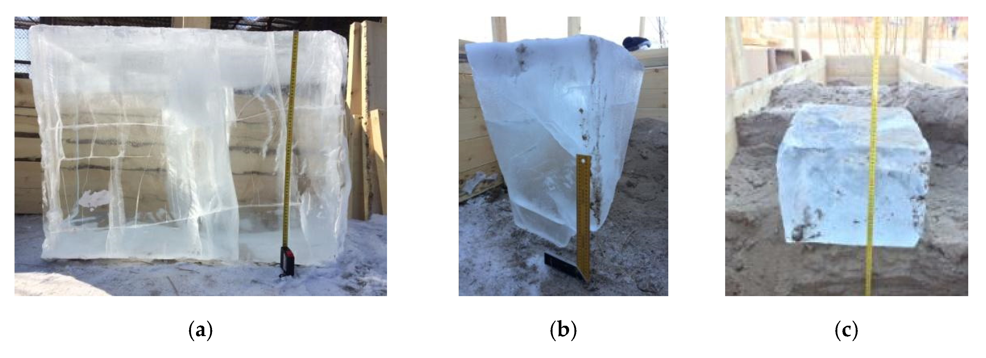
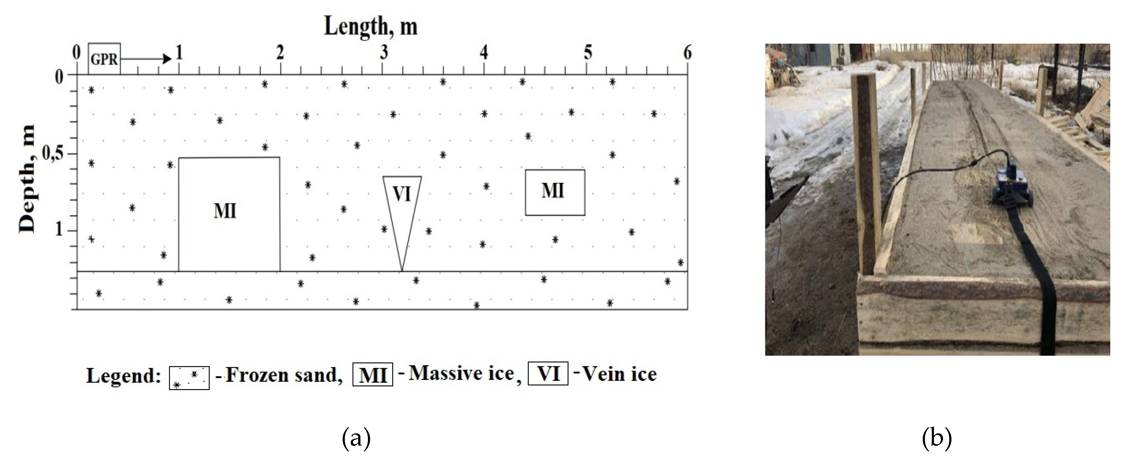
2.4. Physical Simulation of GPR Measurements

For our experiments, we used OKO-2 GPR (LogiS, Russia, detailed information on GPR and antennas can be found on the manufacturer’s official website http://geotechru.com/) with a shielded antenna unit with fc = 1200 MHz. The GPR survey of the model was carried out in a continuous mode and is described below.
For the physical simulation of GPR location of the rock mass with the inclusion of massive ice and ice vein, an installation in the form of a wooden box was built. Ice models were formed from river ice. The dimensions of the first massive ice block: length—1 m, breadth—0.4 m, height—0.73 m (Figure 3a), vein ice: length—0.4 m, breadth—0.37 m, height 0.6 m (Figure 3b) and the second massive ice block: length—0.6 m, breadth—0.4 m, height—0.29 m (Figure 3c).
The installation with dimensions of 6 × 1 × 1.5 m: length—6 m, breadth—1 m, height—1.5 m was located on frozen ground. In the box was host rock, represented by frozen sand with a thickness of 1.25 m with the inclusion of river ice (Figure 4a). On the box, on the outside, marks were made indicating the size and position of the ice. The GPR sounding of the physical model of the frozen rock mass was carried out by two measurement methods—profiling and sounding (Figure 4b). During profiling, the GPR survey was carried out in a continuous mode, the GPR moved along the surface of frozen sand from one edge to the other. The movements of the GPR were recorded on the radargram by marks in accordance with the marks on the outside of the box, which made it possible to know exactly the location of the events of the signals reflected from the ice. When shooting according to the profiling technique, diffracted waves are formed on the radargram, which are reflected waves superimposed, changing their amplitude values. This effect is significant only for small objects compared to the wavelength emitted by GPR, however, to exclude this effect, a survey was also carried out using the sounding technique. In this case, the GPR was located on the surface of frozen sand directly above each ice sample to obtain a GPR trace without extraneous reflections.

3. Results and Discussion

3.1. Computer Simulation

The synthetic radargram obtained as a result of computer simulation is presented in Figure 5b. On GPR traces from 10 to 30 sounding points, a phase change is observed in the signal reflected from the lower boundary (ice-frozen sand) compared to the signal from the upper ice boundary, which corresponds to the negative coefficient of the third term in formula 1 and is displayed on the radargram by a color change from black-and-white-black to white-black-and-white (Figure 5b). The ratio of the amplitudes of the signals reflected from the lower and upper boundaries is calculated for the trace obtained at the 20th sounding point (Figure 5c) Alower/Aupper = 68/84 = 0.8. Let us verify the fulfillment of the condition Alower/Aupper < 0.95∆t: ∆t = tlower − tupper = 10.15 − 6.7 = 3.45 ns and, respectively, 0.953.45 = 0.84 > Alower/Aupper.
Figure 6 shows the Fourier spectra of the traces obtained in the areas with massive ice (Figure 6a) and without it (Figure 6b). The "ripple" shape of the first spectrum is explained by the fact that the ice acts as a comb filter k/Δt (where k = 0, 1, 2 ...), for frequencies multiple of 290 MHz. Since the frequency range in the spectrum is 2500 MHz, N = 2500/290 ≈ 9. In the absence of useful signals (37 s.p.), low-amplitude values with 1 maximum are observed on the Fourier spectrum of the GPR trace.
An example of GPR data obtained by computer simulation for a model with three ice samples from a frozen host medium is shown in Figure 7, which shows the events of the GPR signals reflected from the upper and lower boundaries of the first massive ice. The maxima on the spectral envelope were calculated for each synthetic radargram trace shown in Figure 8. In the areas of the frozen massif model without ice inclusions, the number of maxima is in the range from 1 to 4 (Figure 8), in areas with massive ice from 7 to 15. The graph of maxima allows the determination of the width (1 m) and location of ice with h = 0.72 m. Decreasing the width of ice to 0.6 m leads to a narrowing of the graph, and with a width of 0.42 m, the triangular shape of the graph allows only the suggestion of the presence of massive ice. A large number of maxima (up to 16) characterizes the third ice sample, which is associated with its small thickness h = 0.29 m and, as a result, the presence of a larger number of multiple re-reflections in ice recorded over the interval from 13 ns to 25 ns.

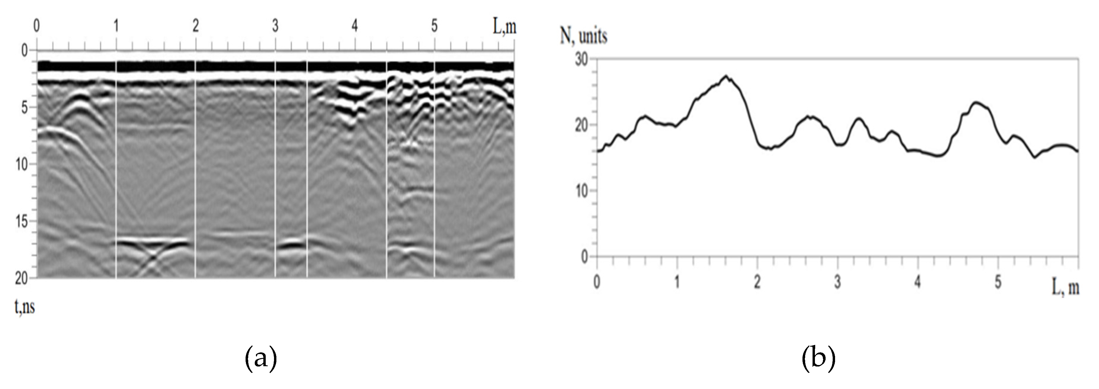
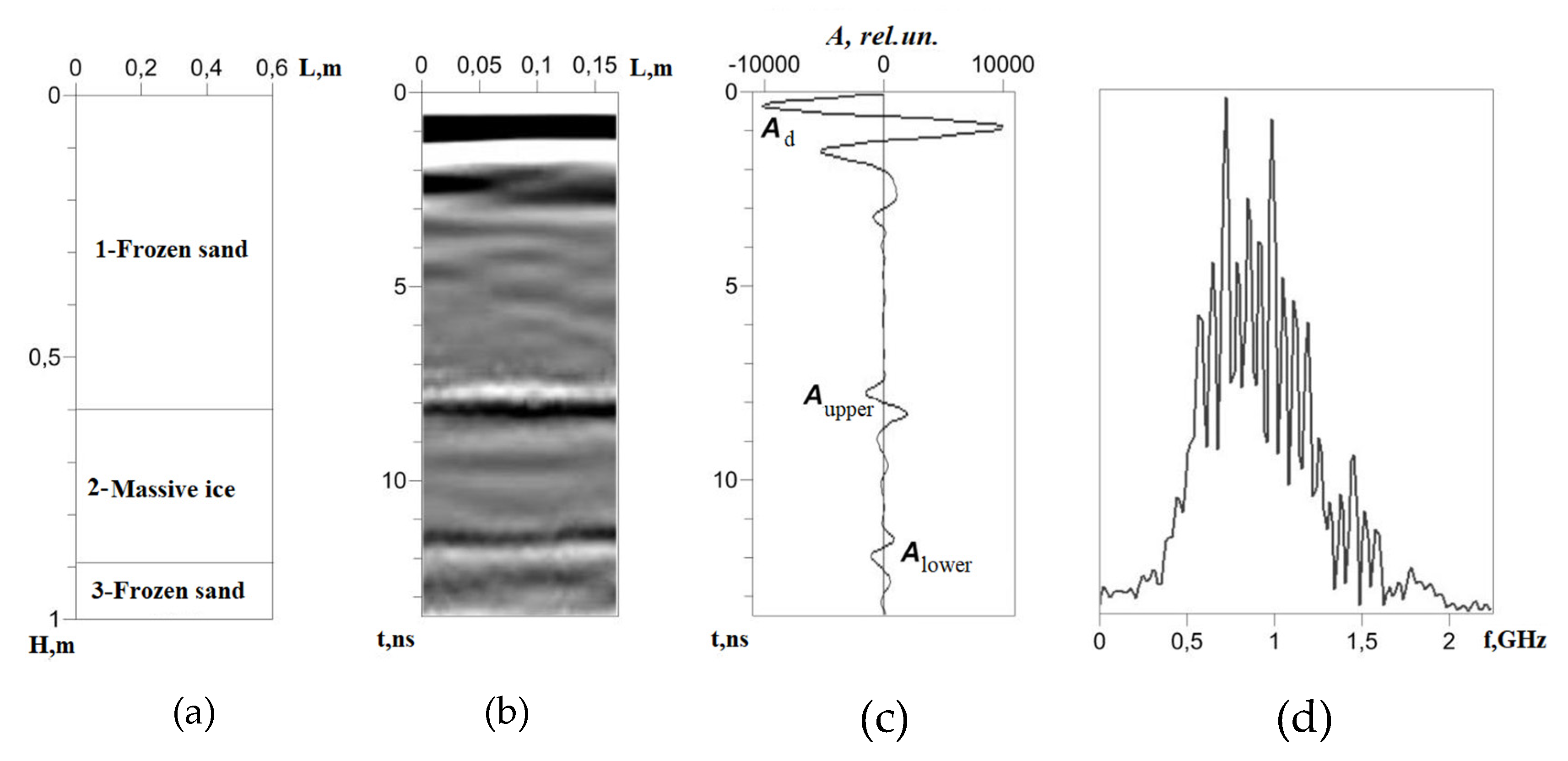
3.2. Physical Simulation

According to the results of GPR measurements on a physical model of frozen rock mass with three ice samples (Figure 4), a radargram was obtained (Figure 9a), in which the white lines indicate the location of ice along the profile. In the wave pattern of the radargram, the events of the reflected waves are traced corresponding to the physical boundaries of the ice. Figure 9b shows the result of calculations of the “ripple” of the Fourier spectrum of the GPR traces of the entire radargram, with averaging of every three points. The figure shows the maxima of the ripple corresponding to the location of massive ice. The remaining maxima located outside the ice zones are formed from interference waves, such as hyperbolic reflections from local objects, diffracted reflections from ice and from the walls of the box, reflections from the roof of frozen ground, and fragmentary reflections from disturbed dumping. However, the maximum vein ice is not confidently detected, since it is at the level of the maxima of the interference waves.
Consider a fragment of a rock mass with the inclusion of massive ice, which is a horizontally layered section (Figure 10a), consisting of layers: 1—a layer of frozen sand with a thickness of 0.6 m; 2—river ice with a thickness of 0.29 m; 3—a layer of frozen sand.
On the processed radargram of the massive ice model, the events of the direct signal and the signals reflected from the physical boundaries of the model layers are determined (Figure 10b). The average signal trace is shown in Figure 10c, on which the amplitude of the direct signal was Ad = −10,835 rel.un. with negative polarity. The signal received at the boundary 1–2 has an amplitude Aupper = −239 rel.un. (tupper = 8 ns) with the same polarity. At the border 2–3, a phase change of the reflected signal with an amplitude of Alower = + 140 rel.un. (tlower = 11.5 ns). Aupper/Alower = 0.6 < 0.953.5 = 0.83. The spectral characteristic of the processed radargram is presented in Figure 10d, which has a rather rugged shape.
Thus, the results of computer and physical simulation confirm the criteria for identifying massive ice in frozen rock mass, established on the basis of the developed model of a single GPR trace. In the general case, given the two-dimensionality of the obtained GPR data, one can formulate the established criteria as follows:
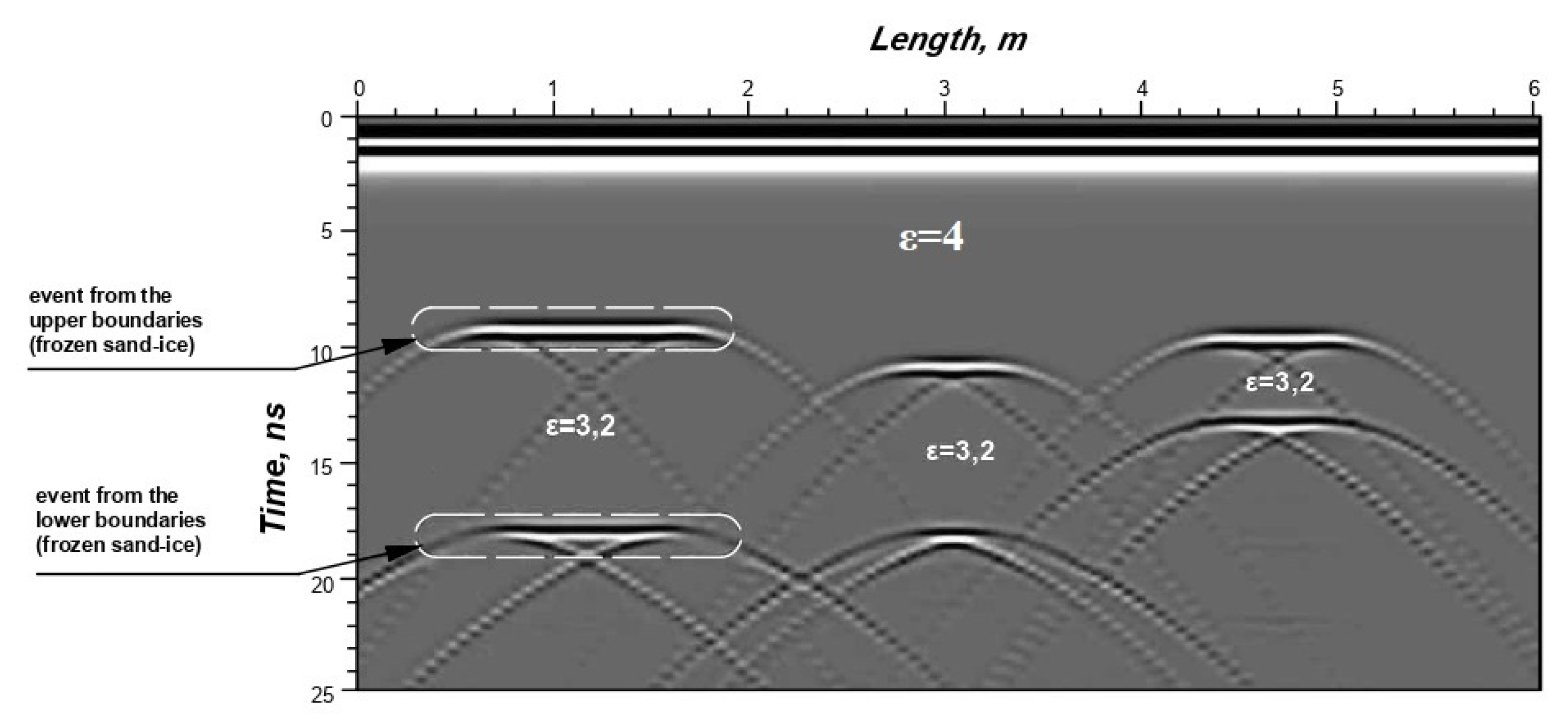
  • the presence of two continuous events of the GPR signals located one below the other;
  • a change in the phase of the signal from the lower ice boundary, compared with the signal from the upper boundary;
  • the Alower/Aupper ratio should be less than 0.95∆t (∆t = tlower − tupper);
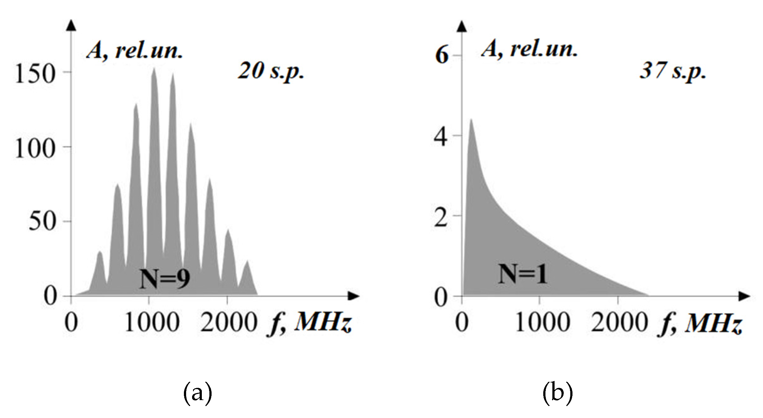
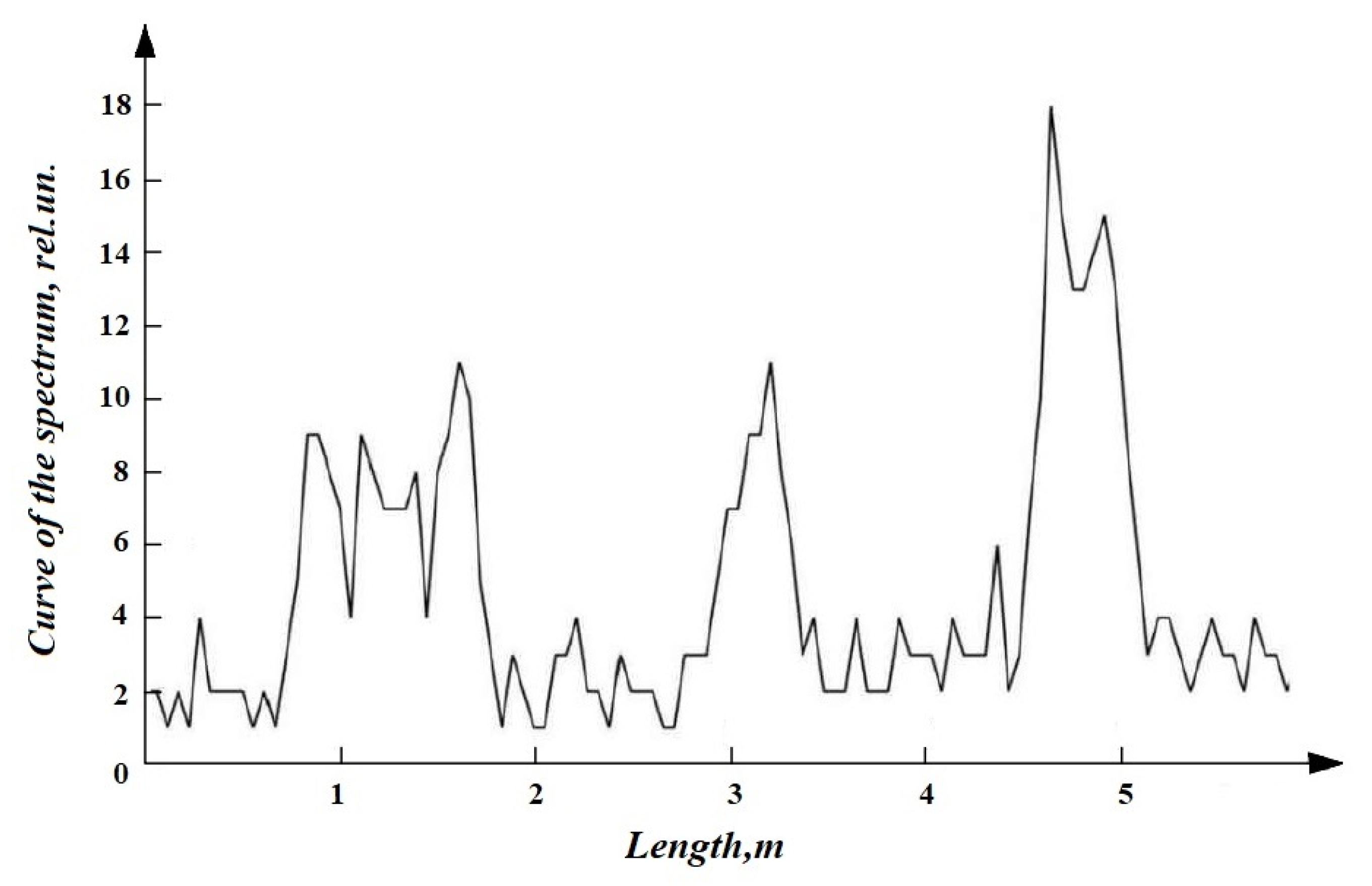
  • increased “ripple” of the envelope of the Fourier spectrum of GPR trace.
After the discovery of massive ice in rock mass or soils for most researchers, the next task is to assess its thickness. Since we know the propagation velocity of electromagnetic waves in ice (vi = 0.168 m/ns), we can determine its thickness (h) by the formula
h = ( t lower t upper ) v л 2 = t 0.084
The value of h calculated by formula (13) allows us to estimate the ice thickness with some accuracy, which depends on various factors. We do not consider the problem of accuracy in determining the thickness of ice, since similar studies have already been conducted [50,51].
In the practical activities of geophysicists, it may be necessary to process large volumes of GPR data obtained, for example, when studying subgrade soils of extensive infrastructure objects (roads, oil and gas pipelines). In such cases, it is better to use existing algorithms for automated processing to determine the values of tlower, tupper [52,53,54,55,56].

4. Conclusions

Our study substantiates the possibility of using GPR for a more detailed study of the structure of permafrost rocks to prevent the appearance of dangerous cryogenic processes in natural and urban areas of the Arctic. For the correct interpretation of GPR radargrams as geophysical data, it is necessary to have sufficiently complete a priori information about the geological and geocryological structure of the studied rock mass. Knowledge of the features of the formation of GPR traces in the study of permafrost can significantly simplify the procedure for interpreting GPR data in the prospecting and evaluation of massive ice and focus on the analysis of patterns of its location.
The results of the analysis of GPR measurements based on the proposed set of features will enable automation of the analysis of large data sets and compile relevant small-scale permafrost-landscape maps with an estimate of the ice thickness for the needs of geocryologists and climatologists.
Currently, the Arctic is undergoing rapid climate change, and an increase in warming is predicted in this region throughout the 21st century. The consequence of this warming will be the intensification of cryogenic processes in a very significant territory (about a quarter of the entire globe). Thawing of permafrost soils and rocks will lead to a deterioration of such operational characteristics of buildings and structures as safety, reliability, maintainability, and durability if appropriate measures are not taken to control them. Using the developed set of features will allow the quick and efficient study of geocryological conditions by GPR, as the basis for monitoring cryogenic processes and taking planning measures to protect infrastructure from the effects of global warming, in order to ensure an acceptable level of life quality for the population in the Arctic.

Author Contributions

Visualization, M.F.; Writing—original draft, K.S.; Writing—review & editing, L.F. All authors have read and agreed to the published version of the manuscript.

Funding

This work was supported by the Russian Foundation for Basic Research, project number 18-45-140061 r_a.

Conflicts of Interest

The authors declare no conflict of interest.

References

  1. Zaikov, K.S.; Kondratov, N.A.; Lipina, S.A.; Bocharova, L.K. Organizational mechanisms for implementing Russia’s Arctic strategy in the 21st century. Arktika Sever 2020, 39, 75–109. [Google Scholar] [CrossRef]
  2. Karjalainen, O.; Aalto, J.; Luoto, M.; Westermann, S.; Romanovsky, V.E.; Nelson, F.E.; Etzmuller, B.; Hjort, J. Circumpolar permafrost maps and geohazard indices for near-future infrastructure risk assessments. Sci. Data 2019, 6, 190037. [Google Scholar] [CrossRef] [Green Version]
  3. Vincent, W.F.; Lemay, M.; Allard, M. Arctic permafrost landscapes in transition: Towards an integrated Earth system approach. Arct. Sci. 2017, 3, 39–64. [Google Scholar] [CrossRef] [Green Version]
  4. Tregubov, O.; Kraev, G.; Maslakov, A. Hazards of activation of cryogenic processes in the Arctic Community: A geopenetrating radar study in Lorino, Chukotka, Russia. Geosciences 2020, 10, 57. [Google Scholar] [CrossRef] [Green Version]
  5. Instanes, A.; Anisimov, O.; Brigham, L.; Goering, D.; Khrustalev, L.N.; Ladanyi, B.; Larsen, J.O. Infrastructure: Buildings, support systems, and industrial facilities. In Arctic Climate Impact Assessment; Symon, C., Arris, L., Heal, B., Eds.; Cambridge University Press: New York, NY, USA, 2005; Chapter 16; pp. 907–944. [Google Scholar]
  6. Ford, J.D.; Bell, T.; St-Hilaire-Gravel, D. Vulnerability of community infrastructure to climate change in Nunavut: A case study from Arctic Bay. In Community Adaptation and Vulnerability in Arctic Regions; Springer Science and Business Media LLC: Berlin/Heidelberg, Germany, 2010; pp. 107–130. [Google Scholar] [CrossRef]
  7. Melvin, A.M.; Larsen, P.; Boehlert, B.; Neumann, J.E.; Chinowsky, P.; Espinet, X.; Martinich, J.; Baumann, M.S.; Rennels, L.; Bothner, A.; et al. Climate damages to Alaska public infrastructure. Proc. Natl. Acad. Sci. USA 2017, 114, E122–E131. [Google Scholar] [CrossRef] [PubMed] [Green Version]
  8. Shiklomanov, N.; Streletskiy, D. Effect of climate change on Siberian infrastructure. In Regional Environmental Changes in Siberia And Their Global Consequences; Springer Environmental Science and Engineering: Dordrecht, The Netherlands, 2013; pp. 155–170. [Google Scholar] [CrossRef]
  9. Harris, C.; Arenson, L.U.; Christansen, H.H.; Etzelmuller, B.; Seppälä, M. Permafrost and climate in Europe: Monitoring and modelling thermal, geomorphological and geotechnical responses. Earth Sci. Rev. 2009, 92, 117–171. [Google Scholar] [CrossRef] [Green Version]
  10. O’Neill, B.; Wolfe, S.; Duchesne, C. New ground ice maps for Canada using a paleogeographic modelling approach. Cryosphere 2019, 13, 753–773. [Google Scholar] [CrossRef] [Green Version]
  11. Zhang, T.; Barry, R.; Knowles, K.; Heginbottom, J.; Brown, J. Statistics and characteristics of permafrost and ground-ice distribution in the Northern Hemisphere. Polar Geogr. 2008, 31, 47–68. [Google Scholar] [CrossRef]
  12. Shpolyanskaya, N.A. Massive ground ice as a basis for paleogeographic reconstruction. In Proceedings of the 8th International Conference on Permafrost, Zurich, Switzerland, 21–25 July 2003; Phillips, M., Springman, S.M., Arenson, L.U., Eds.; A.A. Balkema Publishers: Rotterdam, The Netherlands, 2003. [Google Scholar]
  13. Yoshikawa, K. Notes on open-system pingo ice, Adventdalen, Spitsbergen. Permafr. Periglac. Process. 1993, 4, 327–334. [Google Scholar] [CrossRef]
  14. Fedorov, A.N.; Vasilyev, N.F.; Torgovkin, Y.I.; Shestakova, A.A.; Varlamov, S.P.; Zheleznyak, M.N.; Shepelev, V.V.; Konstantinov, P.Y.; Kalinicheva, S.S.; Basharin, N.I.; et al. Permafrost-landscape map of the Republic of Sakha (Yakutia) on a scale 1:1,500,000. Geosciences 2018, 8, 465. [Google Scholar] [CrossRef] [Green Version]
  15. Brown, J.; Ferrians, O.J.; Heginbottom, J.A., Jr.; Melnikov, E.S. Circum-Arctic Map of Permafrost and Ground-Ice Conditions; Circum-Pacific Map Series CP-45; Geological Survey: Washington, DC, USA, 1997. [Google Scholar]
  16. Tyurin, A.; Isaev, V.; Sergeev, D.; Tumskoi, V.; Volkov, N.; Sokolov, I.; Komarov, O.; Koshurnikov, A.; Gunar, A.; Komarov, I.; et al. Improvement of field methods for engineering geocryological surveying. Mosc. Univ. Geol. Bull. 2019, 74, 70–82. [Google Scholar] [CrossRef]
  17. Zimmerman, R.W.; King, M.S. The effect of freezing on seismic velocities in unconsolidated permafrost. Geophysics 1986, 51, 1285–1290. [Google Scholar] [CrossRef]
  18. Dallimore, S.R.; Davis, J.L. Ground probing radar investigations of massive ground ice and near surface geology in continuous permafrost. GSC 1987, 87–1A, 913–918. [Google Scholar] [CrossRef]
  19. King, M.S.; Zimmerman, R.W.; Corwin, R.F. Seismic and electrical properties of unconsolidated permafrost. Geophys. Prospect 1988, 36, 349–364. [Google Scholar] [CrossRef]
  20. Draebing, D. Application of refraction seismics in alpine permafrost studies: A review. Earth Sci. Rev. 2016, 155, 136–152. [Google Scholar] [CrossRef]
  21. Jørgensen, A.; Andreasen, F. Mapping of permafrost surface using ground-penetrating radar at Kangerlussuaq Airport, western Greenland. Cold Reg. Sci. Technol. 2007, 48, 64–72. [Google Scholar] [CrossRef]
  22. Wollschlager, U.; Gerhards, H.; Yu, Q.; Roth, K. Multi-channel ground-penetrating radar to explore spatial variations in thaw depth and moisture content in the active layer of a permafrost site. Cryosphere 2010, 4, 269–283. [Google Scholar] [CrossRef] [Green Version]
  23. Wang, Y.; Jin, H.; Li, G. Investigation of the freeze–thaw states of foundation soils in permafrost areas along the China–Russia Crude Oil Pipeline (CRCOP) route using ground-penetrating radar (GPR). Cold Reg. Sci. Technol. 2016, 126, 10–21. [Google Scholar] [CrossRef]
  24. Wu, T.; Wang, Q.; Zhao, L.; Du, E.; Wang, W.; Batkhishig, O.; Battogtokh, D.; Watanabe, M. Investigating internal structure of permafrost using conventional methods and ground-penetrating radar at Honhor basin, Mongolia. Environ. Earth Sci. 2012, 67, 1869–1876. [Google Scholar] [CrossRef]
  25. Hauck, C. Frozen ground monitoring using DC resistivity tomography. Geophys. Res. Lett. 2002, 29, 2016. [Google Scholar] [CrossRef]
  26. Hauck, C. New concepts in geophysical surveying and data interpretation for permafrost terrain. Permafr. Periglac. Process. 2013, 24, 131–137. [Google Scholar] [CrossRef] [Green Version]
  27. Kneisel, C.; Hauck, C.; Fortier, R.; Morman, B. Advances in geophysical methods for permafrost investigations. Permafr. Periglac. Process. 2008, 19, 157–178. [Google Scholar] [CrossRef]
  28. Dafflon, B.; Hubbard, S.; Ulrich, C.; Peterson, J.; Wu, Y.; Wainwright, H.; Kneafsey, T. Geophysical estimation of shallow permafrost distribution and properties in an ice-wedge polygon-dominated Arctic tundra region. Geophysics 2016, 81, WA247–WA263. [Google Scholar] [CrossRef]
  29. Munroe, J.S.; Doolittle, J.A.; Kanevskiy, M.Z.; Hinkel, K.M.; Nelson, F.E.; Jones, B.M.; Shur, Y.; Kimble, J.M. Application of ground-penetrating radar imagery for three-dimensional visualization of near-surface structures in Ice-Rich Permafrost, Barrow, Alaska. Permafr. Periglac. Process. 2007, 18, 309–321. [Google Scholar] [CrossRef]
  30. Thomson, L.I.; Osinski, G.R.; Pollard, W.H. Application of the Brewster angle to quantify the dielectric properties of ground ice formations. J. Appl. Geophys. 2013, 99, 12–17. [Google Scholar] [CrossRef]
  31. Watanabe, T.; Matsuoka, N.; Christiansen, H.H. Mudboil and ice-wedge dynamics investigated by electrical resistivity tomography, ground temperatures and surface movements in Svalbard. Geogr. Ann. A 2012, 94, 445–457. [Google Scholar] [CrossRef]
  32. Hinkel, K.M.; Doolittle, J.A.; Bockheim, J.G.; Nelson, F.E.; Paetzold, R.; Kimble, J.M.; Travis, R. Detection of subsurface permafrost features with ground-penetrating radar, Barrow, Alaska. Permafr. Periglac. Process. 2001, 12, 179–190. [Google Scholar] [CrossRef]
  33. Watanabe, T.; Matsuoka, N.; Christiansen, H. Ice- and soil-wedge dynamics in the Kapp Linné Area, Svalbard, investigated by two- and three-dimensional GPR and ground thermal and acceleration regimes. Permafr. Periglac. Process. 2013, 24, 39–55. [Google Scholar] [CrossRef]
  34. De Pascale, G.P.; Pollard, W.H.; Williams, K.K. Geophysical mapping of ground ice using a combination of capacitive coupled resistivity and ground-penetrating radar, Northwest Territories, Canada. J. Geophys. Res. Earth Surf. 2008, 113, F02S90. [Google Scholar] [CrossRef] [Green Version]
  35. Moorman, B.J.; Robinson, S.D.; Burgess, M.M. Imaging Periglacial Conditions with Ground-penetrating Radar. Permafr. Periglac. Process. 2003, 14, 319–329. [Google Scholar] [CrossRef]
  36. Angelopoulos, M.C.; Pollard, W.H.; Couture, N.J. The application of CCR and GPR to characterize ground ice conditions at Parsons Lake, Northwest Territories. Cold Reg. Sci. Technol. 2013, 85, 22–33. [Google Scholar] [CrossRef]
  37. Brandt, O.; Langley, K.; Kohler, J.; Hamran, S. Detection of buried ice and sediment layers in permafrost using multi-frequency Ground Penetrating Radar: A case examination on Svalbard. Remote Sens. Environ. 2007, 111, 212–227. [Google Scholar] [CrossRef]
  38. Yoshikawa, K.; Leuschen, C.; Ikeda, A.; Harada, K.; Gogineni, P.; Hoekstra, P.; Hinzman, L.; Sawada, Y.; Matsuoka, N. Comparison of geophysical investigations for detection of massive ground ice (pingo ice). J. Geophys. Res. 2006, 111. [Google Scholar] [CrossRef] [Green Version]
  39. Shennen, S.; Tronicke, J.; Wetterich, S.; Allrogen, N.; Schwamborn, G.; Schirrmeister, L. 3D ground-penetrating radar imaging of ice complex deposits in northern East Siberia. Geophysics 2016, 81, WA185–WA192. [Google Scholar] [CrossRef] [Green Version]
  40. Hausmann, H.; Behm, M. Imaging the structure of cave ice by ground-penetrating radar. Cryosphere 2011, 5, 329–340. [Google Scholar] [CrossRef] [Green Version]
  41. Annan, A.P.; Davis, J.L. Impulse radar soundings in permafrost. Radio Sci. 1976, 11, 383–394. [Google Scholar] [CrossRef]
  42. Daniels, D. Ground Penetrating Radar, 2nd ed.; The Institution of Electrical Engineers: London, UK, 2004; p. 726. [Google Scholar]
  43. Finkel’shtejn, M.I.; Mendel’son, V.L.; Kutev, V.A. Radiolokacija Sloistyh Zemnyh Pokrovov; Sov. Radio: Moscow, Russia, 1977; p. 167. [Google Scholar]
  44. Benedetto, A.; Pajewski, L. Civil Engineering Applications of Ground Penetrating Radar; Springer: Berlin, Germany, 2015; p. 371. [Google Scholar]
  45. Daniels, D.J. Ground Penetrating Radar; Institution of Engineering and Technology: Stevenage, UK, 2004; p. 761. [Google Scholar]
  46. Hunter, L.E.; Delaney, A.J.; Lawson, D.E.; Davis, L. Downhole GPR for high-resolution analysis of material properties near Fairbanks, Alaska. Geol. Soc. Spec. Publ. 2003, 211, 275–285. [Google Scholar] [CrossRef]
  47. Lapazaran, J.J.; Otero, J.; Martin-Espanol, A.; Navarro, F.J. On the errors involved in ice-thickness estimates I: Ground-penetrating radar measurement errors. J. Glaciol. 2016, 62, 1008–1020. [Google Scholar] [CrossRef] [Green Version]
  48. Harkevich, A.A. Spektry i Analiz; Knizhnyj dom «LIBROKOM»: Moscow, Russia, 2009; p. 240. [Google Scholar]
  49. Warren, C.; Giannopoulos, A.; Giannakis, I. gprMax: Open source software to simulate electromagnetic wave propagation for Ground Penetrating Radar. Comput. Phys. Commun. 2016, 209, 163–170. [Google Scholar] [CrossRef] [Green Version]
  50. Lapazaran, J.J.; Otero, J.; Martin-Espanol, A.; Navarro, F.J. On the errors involved in ice-thickness estimates II: Errors in digital elevation models of ice thickness. J. Glaciol. 2016, 62, 1021–1029. [Google Scholar] [CrossRef] [Green Version]
  51. Onana, V.; Koenig, L.; Ruth, J.; Studinger, M.; Harbeck, J. A semiautomated multilayer picking algorithm for ice-sheet radar echograms applied to ground-based near-surface data. IEEE Trans. Geosci. Remote Sens. 2015, 53, 51–69. [Google Scholar] [CrossRef]
  52. Freeman, G.; Bovik, A.; Holt, J. Automated detection of near surface Martian ice layers in orbital radar data. In Proceedings of the IEEE Southwest Symposium on Image Analysis and Interpretation, Austin, TX, USA, 23–25 May 2010; pp. 117–120. [Google Scholar] [CrossRef]
  53. Ilisei, A.; Bruzzone, L. A model-based technique for the automatic detection of earth continental ice subsurface targets in radar sounder data. IEEE Geosci. Remote Sens. Lett. 2014, 11, 1911–1915. [Google Scholar] [CrossRef]
  54. Ilisei, A.; Bruzzone, L. A system for the automatic classification of ice sheet subsurface targets in radar sounder data. IEEE Geosci. Remote Sens. Lett. 2015, 53, 3260–3277. [Google Scholar] [CrossRef]
  55. Panton, C.; Karlsson, N. Automated mapping of near bed radio-echo layer disruptions in the Greenland Ice Sheet. Earth Planet Sci. Lett. 2015, 432, 323–331. [Google Scholar] [CrossRef] [Green Version]
  56. Ferro, A.; Bruzzone, L. Automatic extraction and analysis of ice layering in radar sounder data. IEEE Trans. Geosci. Remote Sens. 2013, 51, 1622–1634. [Google Scholar] [CrossRef]
Figure 1. Ground-penetrating radar (GPR) model of frozen rock mass with massive ice (a,b) and a schematic diagram of the formation of reflected electromagnetic waves (c).
Geosciences 10 00274 g001
Figure 2. The scheme of a model of frozen rock mass with massive ice.
Geosciences 10 00274 g002
Figure 3. Models of massive ice (a,c) and vein ice (b).
Geosciences 10 00274 g003
Figure 4. The scheme of the rock mass with the inclusion of ice (a) and a photograph of the process of the GPR measurements by the OKO-2 GPR (b).
Geosciences 10 00274 g004
Figure 5. The GPR model of massive ice h = 0.29 m for AB-1200: (a) model of frozen rock mass (FR) with the inclusion of massive ice (MI); (b) radargram; (c) GPR trace.
Geosciences 10 00274 g005
Figure 6. Fourier spectra of the GPR traces of a radargram (Figure 5b) (a) with massive ice; (b) without massive ice.
Geosciences 10 00274 g006
Figure 7. Synthetic radargram of the model (Figure 4a).
Geosciences 10 00274 g007
Figure 8. The result of calculating the “ripple” of the Fourier spectra of GPR traces of the radargram (Figure 7).
Geosciences 10 00274 g008
Figure 9. Radargram of the rock mass with the inclusion of ice (a) and the curve of the spectrum ripple of the GPR signals (b).
Geosciences 10 00274 g009
Figure 10. The scheme of a physical model of massive ice (a) and results of GPR profiling: fragment of a radargram (b), averaged trace (c), spectrum of a radargram (d).
Geosciences 10 00274 g010

