An Analytical Random Field Solution for the Reliability of Axially Loaded Piles in the Ultimate Limit State Considering the Effect of Soil Sampling

Abstract

The present work is concerned with the effect of soil spatial variability on estimating the ultimate soil resistance of floating axially loaded piles from point measurements of soil properties along the pile. The ultimate limit state is considered. In particular, closed form formulae for (i) determining the optimal sampling depth for minimizing statistical uncertainty and (ii) the optimal—minimum required—safety factor for a desired failure probability level are derived. A dimensionless parameter, the cohesion-to-friction parameter Λ, is introduced which quantifies the weight of soil’s cohesion contribution relative to that of soil’s friction in the linear trend of the ultimate soil strength. The analysis shows that the probability of failure profile with the sampling depth attains a minimum, designating the optimal sampling point. This depends on the scaled spatial correlation length of the soil Θ (i.e., the spatial correlation length of soil over the length of the pile) and the parameter Λ, but not on the coefficient of variance of the ultimate soil strength (covu) or the safety factor. Furthermore, it was found that the optimal depth is always at the lower half of the pile, approaching the mid-point or the bottom end of the pile for Λ>>1 or Λ<<1, respectively. In addition, it was found that for large Θ, the optimal depth tends to be closer to the mid-point of the pile, while for small Θ, the optimal sampling depth arises closer to the bottom end. The practical usefulness of the results is related to a suitable choice of the safety factor. Inverting the probability of failure formula at its minimum value, an optimal safety factor is obtained as a function of the desired (acceptable) probability of failure, and the parameters Θ, Λ and covu. The optimal safety factor is the minimum value required for a desired level of the probability of failure.

1. Introduction

While reliability of geotechnical engineering structures is a long-standing problem and a topic of research of major importance, only recently has the research interest focused on statistical uncertainty, i.e., on the effect of targeted field investigation on the reliability of structures. These studies [1,2,3,4,5,6,7,8,9,10,11,12,13,14,15,16,17,18,19,20] aim at finding the sampling location that minimizes statistical error; this location is called “optimal sampling location”. In one of their previous works, the authors [6] studied numerically the effect of targeted field investigation on the reliability of axially loaded piles, aiming at an optimal Serviceability Limit State and Ultimate Limit State design (SLS and ULS, respectively; terms used in Eurocode 7 [21]). Working with the Random Finite Element Method (RFEM) [22] and properly considering sampling in the analysis, they carried out an extensive parametric analysis, considering 5383 different cases. Two sampling strategies were considered: sampling from a single point and sampling from a domain, concluding that statistical uncertainty is greatly affected by both the sampling depth and horizontal distance from the pile and indicating the optimal sampling strategies (the latter are defined by the number and location of the sampling points). Indeed, it has also been shown that the benefit from a targeted field investigation is much greater than the benefit gained using “characteristic” soil property values (such values are used by Eurocode 7 [21]). In the present paper, the problem is studied purely analytically, embedding sampling in an analytical-random field mathematical process. It is mentioned that analytical solutions based on the theory of random fields are generally rare in the geotechnical engineering literature (e.g., [23,24]), whilst according to the best knowledge of the authors, the present one is the first that embeds sampling in an analytical-random field framework.

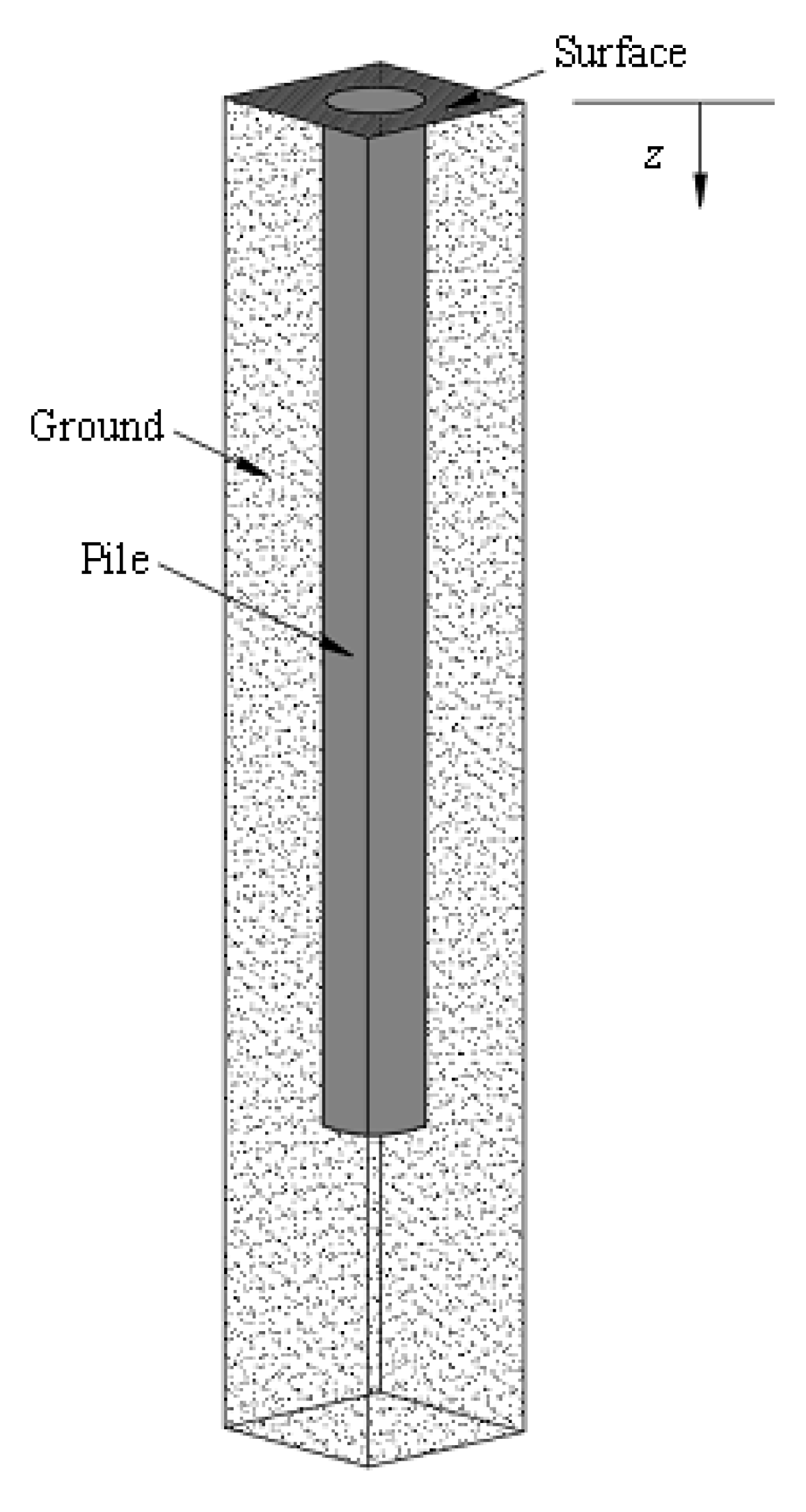
In the analysis that follows, an axially loaded floating pile is assumed, the shaft resistance of which is due to both friction and adhesion. The stiffness of the pile as well as the stiffness of the surrounding soil is regarded as infinite, while the soil has finite strength; this, consequently, refers to an ULS problem (the SLS problem, where the soil has infinite strength, but finite stiffness, is currently under investigation by the authors). The force resisting to the vertical displacement of pile is modeled analytically through a 1D random field with linear trend as a function of depth, representing the ultimate soil strength per unit length. The linear trend models the mean effect of the soil friction and cohesion; the trend is the only input of the mechanics of the soil incorporated in the model. In this respect, the mean values of the soil cohesion and internal friction fields are assumed constant, while the stochastic behavior of the soil cohesion and internal friction contributions to the ultimate soil strength is assumed to be the same (i.e., the correlation function, the correlation length and the coefficient of variation of both contributions is taken to be the same, quantified by a common fluctuations field). It is also mentioned that the internal mechanics of the body of the soil away from the pile is neglected; this is a widely used assumption, especially when the problem is investigated from the 1D numerical point of view (e.g., [25,26,27]). Although this assumption looks crude, it is rather valid as, as shown by Pantelidis [28], the active earth pressure and the at rest earth pressure on a retaining structure are exerted from the same soil wedge; as known, the at rest state of soil is commonly used for the calculation of the shaft resistance of piles due to friction. In addition, Christodoulou et al. [3] showed numerically that the optimal sampling location in the case of retaining walls in the active state is at zero distance from the wall face (the same authors [4] showed that the optimal sampling distance in the problem of retaining walls in the passive state is half wall height away from the wall face). It is, therefore, logical that since the at rest and the active state share the same soil wedge and the optimal sampling location is at zero distance in the active state, the optimal sampling distance in the state at rest to be at the location of the pile.

2. The Random Field of the Ultimate Soil Strength

The ultimate soil strength per unit pile length (in e.g., kN/m) is given by:

$$u=p({{\sigma }^{\prime }}_n\tan {\delta }^{\prime }+{\alpha }_{c}c\prime )=p(1-\sin {\varphi }^{\prime })\tan {\delta }^{\prime }\times \gamma z+p{\alpha }_{c}c\prime$$

(1)

where p is the pile perimeter, δ′ is the pile-soil interface friction angle (usually assumed to be equal to a certain fixed fraction of ϕ′), σ′_n is the normal effective stress on the pile, c′ is the effective cohesion of the soil, and a_c is a soil-pile adhesion factor that depends on c′. σ′_n may be taken to be the lateral earth pressure at rest, i.e., K₀γz = (1 − sinϕ′)γz, where ϕ′ is the internal friction angle of soil, γ the unit weight of the soil and z the depth considered (measured from the surface). The soil is assumed to be normally consolidated. For the sake of simplicity, the effect of the (mobilized) cohesion of soil on the at rest earth pressure coefficient (see Pantelidis [28]) has been neglected, although for axially loaded piles this effect is unfavorable. The adhesion factor is usually mentioned in the literature in the undrained type of analysis (e.g., Das [29]), however, in the present paper, it is mentioned in the general case. Drained soil conditions could be regarded, taking ϕ_u = 0 and cohesion equal to c_u instead of ϕ′ and c′, respectively.

The quantities ϕ′ and c′ will be regarded as random fields along the length of the pile which have the same value around the perimeter of the pile at every depth z. Hence, they are 1D random fields varying only along the pile length (Figure 1).

For the sake of simplicity, each one of the grouped quantities p(1 − sinϕ′)tanδ′ and pa_cc′ shall be modeled by a random field. It is plausible that these random fields have similar stochastic properties, differing only in the expectation values. That means that these fields can be modeled in terms of a single random field, as follows:

$$p(1-\sin {\varphi }^{\prime })\tan {\delta }^{\prime }=p(1-\sin \overline{{\varphi }^{\prime }})\tan \overline{{\delta }^{\prime }}(1+{\mathrm{cov}}_u\omega (z)),$$

(2)

$$p{\alpha }_c{c}^{\prime }=p{\alpha }_{\overline{c}}{\overline{c}}^{\prime }(1+{\mathrm{cov}}_u\omega (z)),$$

(3)

where cov_u is the (common) coefficient of variance of each one of the two fields and, hence, the coefficient of variance value of the ultimate soil strength per unit length u; the random field ω(z) is the fluctuations field, which is a Gaussian field of zero mean and unit variance, exhibiting Markovian (linear exponential) correlations:

$$E[\omega (z)\omega (z^{\prime })]=\exp \left[-\frac{2\left|z-z^{\prime }\right|}{\theta }\right]$$

(4)

E[…] is the expectation value operator. The quantity θ is the correlation length of the fluctuations of the field ω, and hence of the fields p(1 − sinϕ′)tanδ′ and pα_cc′. In all, the quantities cov_u and θ and the form of the function given in Equation (4) encode the common stochastic structure assumed for the fields p(1 − sinϕ′)tanδ′ and pα_cc′. Finally, the possible change of the expectation values of these fields with the depth shall be neglected. Hence, the expectation values, denoted by an overbar, will be assumed constant.

Forming now the field u by Equations (1)–(3) one obtains:

$$u=\overline{u}\left(1+{\mathrm{cov}}_u\omega \right),$$

(5)

with the expectation value $\overline{u}$ given by:

$$\overline{u}=p(1-\sin \overline{{\varphi }^{\prime }})\tan \overline{{\delta }^{\prime }}\times \gamma z+p{\alpha }_{\overline{c}}{\overline{c}}^{\prime }.$$

(6)

It can, easily, now be shown that the quantity designated as cov_u is indeed the coefficient of variance of the ultimate soil strength (per unit pile length) field u. The linear trend of the expectation value $\overline{u}$ of the ultimate strength per unit length is of high importance in this work.

Given that eventually the probability of failure shall be calculated, which is a dimensionless quantity, its dependence on the parameters of the problem will be realized through dimensionless quantities. An important quantity is the ratio:

$$\Lambda =\frac{{\alpha }_{\overline{c}}{\overline{c}}^{\prime }}{(1-\sin \overline{{\varphi }^{\prime }})\tan \overline{{\delta }^{\prime }}\gamma L},$$

(7)

where L is the pile length. The ratio Λ is the relative weight of the cohesion and friction terms in linear trend of the ultimate soil strength, given in Equation (6) (it is called hereafter cohesion-to-friction parameter). Then the trend can be written as:

$$\begin{array}{r}\overline{u}=A\left(\frac{z}{L}+\Lambda \right)\hfill \\ A:=p(1-\sin \overline{{\varphi }^{\prime }})\tan \overline{{\delta }^{\prime }}\times \gamma L\hfill \end{array}\},$$

(8)

where A is a quantity defined for algebraic convenience. Equivalently, employing explicitly the values of the trend at top and bottom end of the pile length, the trend of the ultimate soil strength can be written as:

$$\begin{array}{r}\overline{u}=({\overline{u}}_{\mathrm{bottom}}-{\overline{u}}_{\mathrm{top}})\frac{z}{L}+{\overline{u}}_{\mathrm{top}}\hfill \\ \\ {\overline{u}}_{\mathrm{top}}=A\Lambda \hfill \\ {\overline{u}}_{\mathrm{bottom}}=A(1+\Lambda )\hfill \end{array}\},$$

(9)

which means that:

$$\frac{{\overline{u}}_{\mathrm{bottom}}}{{\overline{u}}_{\mathrm{top}}}=\frac{1+\Lambda }{\Lambda }.$$

(10)

The large values of Λ correspond to relatively strong cohesion contribution and a nearly uniform trend; inversely, small values of Λ correspond to relatively strong friction contribution, and the trend exhibits a large slope.

From these data the statistics of the (total) ultimate soil strength $U$ [kN] can be calculated:

$$U={\displaystyle {\int }_0^{L}udz}.$$

(11)

The latter, using Equations (5) and (8) becomes:

$$\begin{array}{ll}\hfill U& ={\displaystyle {\int }_0^{L}u dz}=A{\displaystyle {\int }_0^L\left(\frac{z}{L}+\Lambda \right)}(1+{\mathrm{cov}}_u\omega (z))dz\hfill \\ & =\overline{U}+{\mathrm{cov}}_{u}A{\displaystyle {\int }_0^L\left(\frac{z}{L}+\Lambda \right)}\omega (z)dz\hfill \\ & =\overline{U}+\overline{U}\frac{{\mathrm{cov}}_u}{\frac{1}{2}+\Lambda }{\displaystyle {\int }_0^L\left(\frac{z}{L}+\Lambda \right)}\omega (z)\frac{dz}{L}\hfill \end{array},$$

(12)

where, based on Equations (8) and (11):

$$\overline{U}=AL\left(\frac{1}{2}+\Lambda \right).$$

(13)

$U$ (recall Equation (12)) is a superposition of Gaussian random variables. Hence, it is Gaussian random variable itself and it is completely defined by its mean $\overline{U}$ and standard deviation. σ_U, or equivalently, is its coefficient of variation. Using Equations (4) and (12), the (squared) coefficient of variation of $U$ reads:

$$\frac{E[{(U-\overline{U})}^2]}{{\overline{U}}^2}=\frac{{\mathrm{cov}}_u^2}{{\left(\frac{1}{2}+\Lambda \right)}^2}{\displaystyle {\int }_0^L{\displaystyle {\int }_0^L\left(\frac{z}{L}+\Lambda \right)\left(\frac{z^{\prime }}{L}+\Lambda \right)\exp \left[-\frac{2\left|z_1-z_2\right|}{\theta }\right]\frac{dzd{z}^{\prime }}{L^2}}}.$$

(14)

The calculation of the integrals is relatively straightforward. One finds:

$$\frac{E[{(U-\overline{U})}^2]}{{\overline{U}}^2}={\mathrm{cov}}_u^2{\left(\frac{1}{2}+\Lambda \right)}^{-2}\times \left\{\begin{array}{l}\left(\frac{1}{3}\Theta -\frac{1}{4}{\Theta }^2+\frac{1}{8}{\Theta }^4-\frac{1}{4}{\Theta }^3{e}^{-2/\Theta }-\frac{1}{8}{\Theta }^4{e}^{-2/\Theta }\right)\\ +\Lambda \left(\Theta -\frac{1}{2}{\Theta }^2+\frac{1}{2}{\Theta }^2{e}^{-2/\Theta }\right)+{\Lambda }_{}^2\left(\Theta -\frac{1}{2}{\Theta }^2+\frac{1}{2}{\Theta }^2{e}^{-2/\Theta }\right)\end{array}\right\},$$

(15)

where:

$$\Theta =\theta /L.$$

(16)

is the scaled correlation length.

3. Design Ultimate Soil Strength from Sampling

Measuring the fields ϕ′ and c′ at any depth z = z_s in the vicinity of the pile will provide an estimate for the soil ultimate strength, $U_s$, as follows. The stochasticity of the field u is carried—in the present paper—by the fluctuations field ω(z), which encodes the (common) stochastic properties of the fluctuations of the friction and cohesion random fields. A measurement at a depth z = z_s picks a value ω(z_s) of the field ω. The value ω(z_s) is a random variable modeling the stochastic nature of the measurement. Then the estimated ultimate soil strength reads as:

$$U_s=A{\displaystyle {\int }_0^L\left(\frac{z}{L}+\Lambda \right)}\left(1+{\mathrm{cov}}_u\omega \left(z_s\right)\right)dz=\overline{U}\left(1+{\mathrm{cov}}_u\omega \left(z_s\right)\right)$$

(17)

using Equation (8). Clearly, this is a Gaussian random variable. Its expectation value is:

$$\overline{U_s}=\overline{U}$$

(18)

as the fluctuations field ω has zero expectation value. Also, by Equation (4), the (squared) coefficient of variation of U_s is:

$$\frac{E[{(U_s-\overline{U})}^2]}{{\overline{U}}^2}={\mathrm{cov}}_u^2$$

(19)

These data define completely the random variable U_s.

4. Probability of Failure

Given an estimate $U_s$ for the total ultimate soil strength, the limiting load Q is designated as $U_s/F$ for a certain factor of safety F. The probability of failure is defined as:

$$PF=\mathrm{Probability}\left(U<\frac{U_s}{F}\right).$$

(20)

Defining:

$$Z=U-\frac{U_s}{F},$$

(21)

a random variable is obtained, which is also Gaussian, as a superposition of Gaussian random variables. Therefore:

$$PF=\mathrm{Probability}\left(Z<0\right)=\Phi \left(-\frac{\overline{Z}}{{\sigma }_Z}\right)=\Phi \left(-\frac{1}{{\mathrm{cov}}_Z}\right).$$

(22)

where Φ is the probability function of the normalized normal distribution. The mean value of Z reads as:

$$\overline{Z}=\overline{U}\left(1-\frac{1}{F}\right),$$

(23)

while its (squared) coefficient of variation reads as:

$$\begin{array}{ll}\hfill {\mathrm{cov}}_Z^2& =\frac{E[{(Z-\overline{Z})}^2]}{{\overline{Z}}^2}={\left(1-\frac{1}{F}\right)}^{-2}\frac{1}{{\overline{U}}^2}E\left[{\left(U-\overline{U}-\frac{U_s-\overline{U}}{F}\right)}^2\right]\hfill \\ & ={\left(1-\frac{1}{F}\right)}^{-2}\left[\frac{E[{(U-\overline{U})}^2]}{{\overline{U}}^2}-\frac{2}{F}\frac{E[(U-\overline{U})(U_s-\overline{U})]}{{\overline{U}}^2}+\frac{1}{F^2}\frac{E[{(U_s-\overline{U})}^2]}{{\overline{U}}^2}\right]\hfill \end{array}.$$

(24)

The first and last term in the square brackets correspond to the coefficient of variation of the variables $U$ and $U_s$, given by Equations (15) and (19). The middle term corresponds to the correlation coefficient between the soil strength U and the estimated soil strength $U_s$ from a measurement at a depth z_s. It reads as:

$$\begin{array}{ll}\hfill \frac{E[(U-\overline{U})(U_s-\overline{U})]}{{\overline{U}}^2}& =-\frac{2}{F}\frac{{\mathrm{cov}}_u^2}{\left(\frac{1}{2}+\Lambda \right)}{\displaystyle {\int }_0^L\left(\frac{z}{L}+\Lambda \right)\exp \left[-\frac{2\left|z-z_s\right|}{\theta }\right]}\frac{dz}{L}\hfill \\ & =\frac{{\mathrm{cov}}_u^2}{\frac{1}{2}+\Lambda }\left\{\begin{array}{l}\frac{1}{4}\Theta \left(\Theta -2\Lambda \right)e^{-2\zeta /\Theta }\\ -\frac{1}{4}\Theta \left(\Theta +2\Lambda +2\right)e^{-2(1-\zeta )/\Theta }+\left(\zeta +\Lambda \right)\Theta \end{array}\right\}\hfill \end{array},$$

(25)

where Equations (4), (12) and (17) have been used; the dimensionless depth ζ of the observation point has been defined as:

$$\zeta =z_s/L.$$

(26)

Clearly, this term encodes the effect of sampling on the design.

In all, by Equations (15), (19), (22) and (25), the cov value of the random variable Z is:

$$\begin{array}{ll}\hfill {\mathrm{cov}}_Z^2& =\frac{{\mathrm{cov}}_u^2}{{\left(1-\frac{1}{F}\right)}^2}\left(T_1-\frac{2}{F}{T}_2+\frac{1}{F^2}\right)\hfill \\ \\ \hfill T_1:& =\frac{1}{{\left(\frac{1}{2}+\Lambda \right)}^2}\times \left\{\begin{array}{l}\left(\frac{1}{3}\Theta -\frac{1}{4}{\Theta }^2+\frac{1}{8}{\Theta }^4-\frac{1}{4}{\Theta }^3{e}^{-2/\Theta }-\frac{1}{8}{\Theta }^4{e}^{-2/\Theta }\right)\\ +\Lambda \left(\Theta -\frac{1}{2}{\Theta }^2+\frac{1}{2}{\Theta }^2{e}^{-2/\Theta }\right)+{\Lambda }_{}^2\left(\Theta -\frac{1}{2}{\Theta }^2+\frac{1}{2}{\Theta }^2{e}^{-2/\Theta }\right)\end{array}\right\}\hfill \\ \hfill T_2:& =\frac{1}{\frac{1}{2}+\Lambda }\left\{\frac{1}{4}\Theta \left(\Theta -2\Lambda \right)e^{-2\zeta /\Theta }-\frac{1}{4}\Theta \left(\Theta +2\Lambda +2\right)e^{-2(1-\zeta )/\Theta }+\left(\zeta +\Lambda \right)\Theta \right\}\hfill \end{array}\}.$$

(27)

The quantities T₁ and T₂ essentially correspond to suitable dimensionless forms of the three terms in Equation (24) and depend only on Θ and Λ, which are both dimensionless. Evaluating cov_Z immediately provides the probability of failure PF by Equation (22).

5. Optimal Sampling Depth

The optimal sampling depth is defined as the depth along the pile where the probability of failure PF, given by Equations (22) and (27), attains a minimum, for given values of the parameters Θ, Λ, and F. Note that the sampling depth appears only in the correlation term in Equation (24) as explained above, that is, in the T₂ term (recall Equation (27)). In that term, the safety factor F appears only as an overall factor, hence the optimal sampling depth is independent of F. Given also that cov_u is an overall factor in Equation (27), the optimal sampling depth is also independent of that value (as long as it is not zero).

Differentiating cov_Z with respect to ζ and setting the result to zero:

$${\zeta }_{\mathrm{optimal}}=-\frac{\Theta }{2}\ln \left[\frac{\Theta -e^{-1/\Theta }\sqrt{4\Lambda (1+\Lambda )-2\Theta -{\Theta }^2+{\Theta }^2{e}^{2/\Theta }}}{\Theta -2\Lambda }\right].$$

(28)

In the large Θ limit, that is, in the limit where the entire field becomes a single uniform random variable, the optimum sampling depth takes the form

$${\zeta }_{\mathrm{optimal}}=\sqrt{{\Lambda }_{}^2+\Lambda +\frac{1}{2}}-\Lambda .$$

(29)

On the other hand, in the limit of very small correlations lengths, Θ → 0:

$${\zeta }_{\mathrm{optimal}}=1.$$

(30)

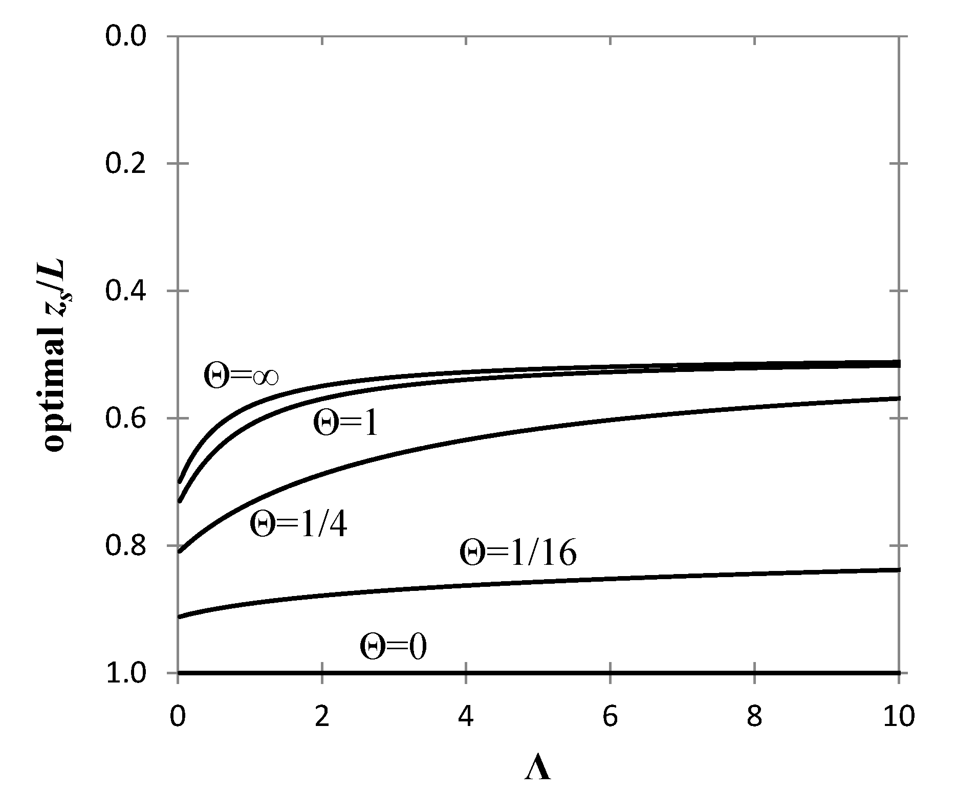
It is important to note that in the limit of small variability (large Θ), the minimum of the probability of failure becomes very shallow and it is of no practical importance. The usefulness of Equations (29) and (30) is that they provide the two ends of the possible optimal depths for given Λ. Figure 2 shows the optimal sampling depth given by Equation (28) as a function of Λ for different correlation lengths. From these curves, one deduces the following:

• The optimal sampling depth becomes less sensitive to the parameter Λ, as Θ tends to zero.
• The optimal sampling depth is always at the lower half of the pile.
• For Λ values much smaller than unity, the optimal sampling location lies at depth greater than 0.7 × L.
• For small Θ values, i.e., Θ << 1, the optimal sampling depth lies near the bottom end of the pile, although as it is clarified below, the notion of optimality is weakened in the limit of very small Θ.

6. Analysis of the Probability of Failure

The dependence of the probability of failure on the parameters Θ, Λ, and F is investigated in this section. Such an analysis will further clarify the nature and the properties of the optimal sampling depth discussed above.

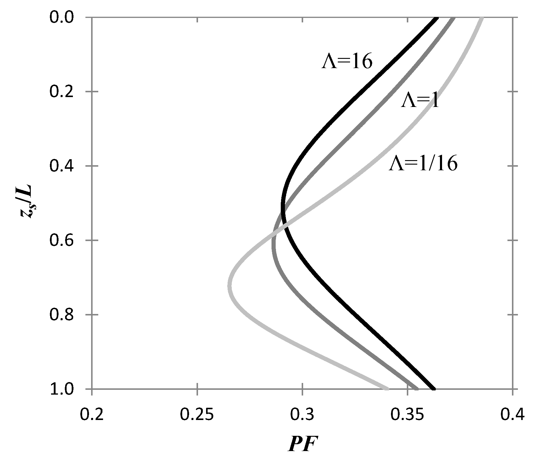
Figure 3 shows the profile of the probability of failure with respect to the normalized sampling depth, z_s/L, for Λ = 1/16, 1 and 16 (values corresponding to weak, intermediate and strong cohesion respectively). For all curves it stands that F = 1.1, cov_u = 1/3, and Θ = 1. The curves reveal the transformation of the PF profile with increasing adhesion, and in particular the displacement of the optimal sampling point to shallower depths. Clearly, this result is emphasized further with the remarks of the previous section and Figure 2.

Figure 4 illustrates the effect of the correlation length on the profile of the probability of failure for sampling along the pile. For all curves, it stands that F = 1.1, cov_u = 1/3, and Λ = 1. As it is inferred from the figure in question, for large correlation lengths, the optimal sampling point arises at smaller depths, towards the mid-point of the pile, while the minimum of the PF becomes shallower. The reason is that in the limit Θ → ∞, the spatial variability vanishes. Trivially, PF becomes independent of z_s. Using Equation (27) it can easily be shown that in this limit:

$${\mathrm{cov}}_Z={\mathrm{cov}}_u.$$

(31)

Indeed, for the values of the parameters used for the curves of Figure 3, cov_Z = 1/3, which implies PF = 0.00135 (recall Equation (22)).

In the limit of very small correlation lengths, the minimum arises at larger depths, towards the lowermost point of the pile, while the minimum of the PF becomes again shallower. The reason is that in the limit of very small correlation length, the values of the random field u at different points become independent, hence any notion of location along the pile is lost; mathematically, the limit Θ = θ/L → 0, means that the length L is infinitely larger as compared to the correlation length θ of soil. Hence, the probability of failure is independent of the sampling point. The difference with the case of large Θ, is that the PF in this case is not zero. Indeed, Equation (27) implies that in the limit Θ → 0

$${\mathrm{cov}}_Z=\frac{{\mathrm{cov}}_u}{F-1}.$$

(32)

For the values of the parameters used for drawing the curves of Figure 4, it stands that cov_Z = 3.3, which implies PF = 0.38 (recall Equation (22)).

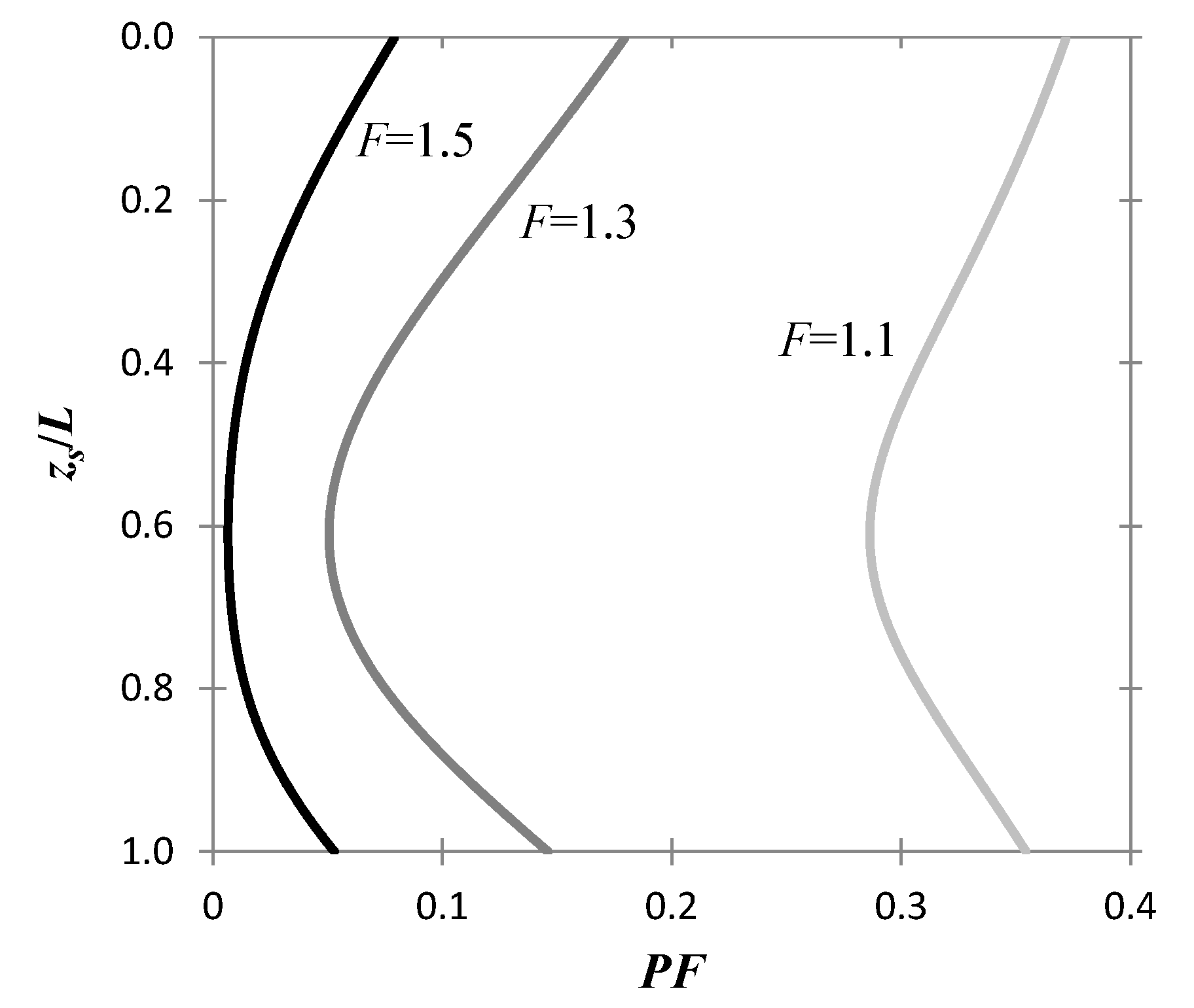
Finally, the effect of the safety factor F is illustrated in the PF versus z_s/L chart of Figure 5, where different F values were used, i.e., F = 1.1, 1.3, and 1.5. The chart in question refers to cov_u = 1/3, Θ = 1, and Λ = 1. The curves of Figure 5 indicate that as F increases, the probability of failure, as expected, decreases, while for a certain safety factor value, the optimal depth is the center of an interval of depths where the associated PF is significantly smaller than the PF outside that interval.

Another interesting observation that can be made based on Figure 5 is that there is a F value for which the difference between the maximum and minimum PF value on the PF versus z_s/L chart becomes maximum. This safety factor value is called, thereafter, optimal safety factor value (this is subject matter of the following section).

7. The Optimal Safety Factor Value

The goal in this section is to define the required safety factor value for absorbing statistical uncertainty in an explicit manner which is optimal in the sense that it corresponds to the target (acceptable) failure probability. The required safety factor value is, apparently, the minimum possible; thus, this value guarantees the desired level of reliability in the most cost-effective manner (referring to statistical uncertainty, only).

In this respect, defining the z score corresponding to a desired probability of failure PF by

$$\Phi (z_{PF})=PF,$$

(33)

and using the standard property $z_{1-PF}=-z_{PF}$ it stands that by Equation (22):

$${\mathrm{cov}}_Z=\frac{1}{z_{1-PF}}.$$

(34)

Then, from Equation (27):

$${\left(1-\frac{1}{F}\right)}^2=z_{1-PF}^2{\mathrm{cov}}_u^2\left(T_1-\frac{2}{F}{T}_2+\frac{1}{F^2}\right),$$

(35)

where the magnitudes T₁ and T₂ have already been defined in Equation (27). Solving the latter as for F:

$$\begin{array}{ll}\hfill F_{PF}& =\frac{1-Y{T}_2+\sqrt{Y(1+T_1-2T_2+Y(T_2^2-T_1))}}{1-Y{T}_1}\hfill \\ \hfill Y:& =z_{1-PF}^2{\mathrm{cov}}_u^2\hfill \end{array}\}.$$

(36)

The parameter Y carries the dependence of F_PF on both the level of the probability PF of failure and cov_u which do not appear in the quantities T₁ and T₂. Now, if PF refers to the optimal sampling point, the F_PF (that is, the safety factor for a given level of failure probability) can be calculated in terms of the parameters Θ, Λ, and cov_u. One should recall that the optimal depth is given by Equation (28). Then, F_PF is the minimum required safety factor to achieve the desired probability of failure (optimal safety factor value for the given probability of failure). For example, consider a 15 m pile with 25 cm perimeter, embedded in uniform clay with the following properties: γ = 18 kN/m³, ϕ′ = 30°, c′ = 30 kN/m². We may take a_c = 0.8 and δ′ = (0.8)∙30° = 24° (Das [29]). The correlation length θ for clay may be taken 0.20m (see e.g., Pantelidis and Christodoulou [30]; in the paper in question, the θ value of two clay fields in Cyprus was calculated using the more convenient Fluctuation Function Method. A comparative assessment of the methods-of-moments for estimating the correlation length of one-dimensional random fields can be found in [31]). For a probability of failure PF = 0.0001, the minimum safety factor F_PF is estimated 2.3.

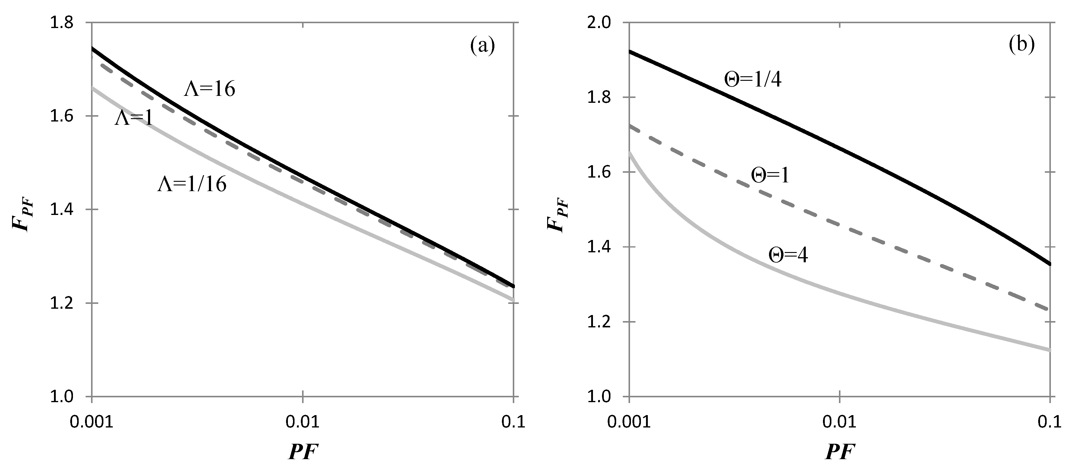
In Figure 6, the safety factor F_PF is plotted against the desired PF value in the range 0.001 to 0.1 for (a) different values of Λ, setting cov_u = 1/3 and Θ = 1, and (b) different Θ values, setting Λ = 1 and cov_u = 1/3. The dashed line in both charts corresponds to Θ = 1, Λ = 1 and cov_u = 1/3. From Figure 6a it is inferred that the optimal safety factor increases as cohesion increases or friction decreases (that is, as Λ increases) and vice versa. That means that a design is safer if it mostly relies on friction. Figure 6b shows the influence of Θ on the optimal safety factor. In this respect, small correlation lengths, i.e., more spatially variable soils, require higher safety factor for any given desired probability of failure and vice versa.

8. Comparison with RFEM

In this section, the Random Finite Element Method (RFEM) is employed in order the optimal sampling depth to be investigated and to the results to be set against the respective ones of Equations (22) and (27). The freely available RFEM program RPILE1D [32] (http://www.engmath.dal.ca/rfem) has been extended by the authors [6] to allow for the consideration of sampling in the analysis. The RPILE1D program is described in detail in [32], so only a brief description is given here. The pile is divided into a series of elements, with a certain axial stiffness, related to the pile modulus of elasticity. Moreover, the soil spring elements, which are attached to the nodes, are characterized by their initial stiffness and their ultimate strength (bilinear relationship; see [22]). The initial stiffness is a function of the modulus of elasticity of the soil, while the ultimate strength is given by Equation (1). Hence, the RFEM model consists of three 1D random fields: the spring stiffness and spring strength contributions from the soil per unit length along the pile, and the stiffness of the pile. These fields are log-normally distributed [32],while they have the same spatial correlation length and the same type of correlation function (Markovian).

The original RPILE1D program returns the load in each simulation beyond which the given maximum settlement (δ_max) becomes intolerable or the ultimate load that the pile can carry just prior to failure. These two loads correspond to the serviceability and ultimate limit state, respectively (SLS and ULS). The ULS state (which is examined in the present paper) is defined by the sum of the ultimate strength (U_s) over all the springs. The modified RPILE1D program [6] returns the probability of failure based on soil stiffness and ultimate strength values sampled from various depths of the respective 1D random fields along the pile. More specifically, the probability of failure is defined by the fraction of the realizations resulted in failure over the total number of realizations. In each realization, ‘failure’ is considered to have occurred when the calculated shaft resistance of pile considering spatially uniform properties sampled from the soil divided by a factor of safety is greater than the respective one considering spatially random properties.

The original RPILE1D program returns the load in each simulation beyond which the given maximum settlement (δ_max) becomes intolerable or the ultimate load that the pile can carry just prior to failure. These two loads correspond to the serviceability and ultimate limit state, respectively (SLS and ULS). The ULS state (which is examined in the present paper) is defined by the sum of the ultimate strength (U_s) over all the springs. The modified RPILE1D program [6] returns the probability of failure based on soil stiffness and ultimate strength values sampled from various depths of the respective 1D random fields along the pile. More specifically, the probability of failure is defined by the fraction of the realizations resulted in failure over the total number of realizations. In each realization, ‘failure’ is considered to have occurred when the calculated shaft resistance of pile considering spatially uniform properties sampled from the soil divided by a factor of safety is greater than the respective one considering spatially random properties.

Allowing for a direct comparison between the RFEM method and the respective analytical work of this paper, the RPILE1D program presented by Christodoulou et al. [6] was further modified as to (i) consider normal distributions (in addition to the log-normal ones already considered by the original program) and (ii) distinguish sampling cohesion values of soil from sampling internal friction values of soil, since both contribute to the ultimate soil resistance as described by Equation (1). Both modifications have been made so that the program to be consistent with the sampling procedure of the analytical model discussed in the previous sections.

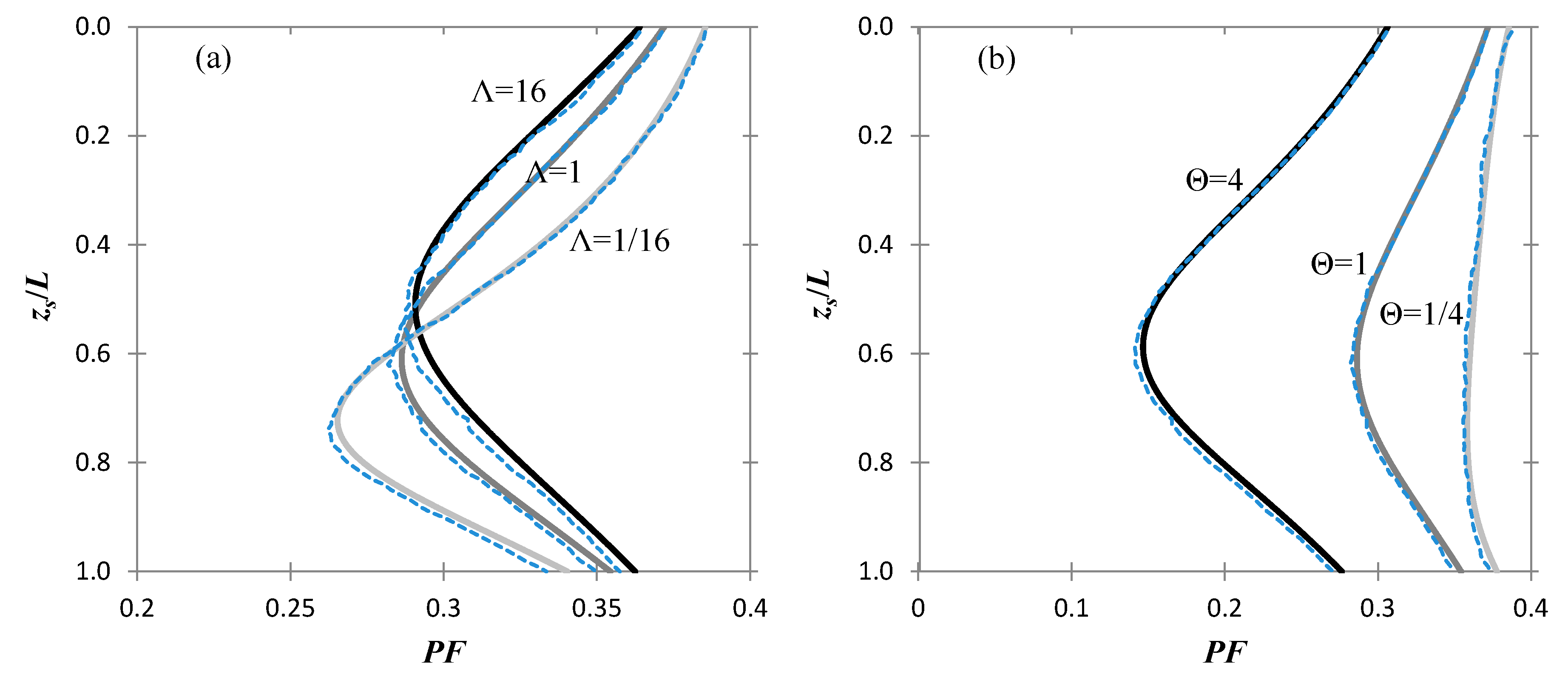
In Figure 7 the probability of failure profiles as a function of the sampling depth are shown for different values of the Λ ratio (Figure 7a) and different Θ values (Figure 7b); the analytical results are represented by continuous lines, while the RFEM results by dashed lines. For consistency between the numerical and the analytical modeling, the pile and soil stiffness of the RFEM models was set as very large, as in the theoretical setup of Section 2, the pile is regarded as rigid and the soil resistance is solely given by the soil strength u. Moreover, the coefficient of variance of u was set to 1/3, while the safety factor F was set to 1.1, in both the numerical and the analytical analyses. Figure 7a, refers to Θ = θ/L = 1, while Figure 7b to Λ = 1. Regarding the cohesion-to-friction parameter Λ, the actual numerical input in the RFEM model is the top and bottom (of side of the pile) values of the ultimate strength u related to Λ by Equation (10). Specifically, u_top was equal to 10 kN/m, while u_bottom was equal to 170, 20, 10.625 kN/m for Λ = 1/16, 1 and 16, respectively, although any top and bottom ratio of values that produces the same Λ gives the same probability of failure. It is also noted that the analysis by Christodoulou et al. [6] corresponds to the case of Λ = ∞. Finally, for producing smooth numerical curves, the number of realizations was set to 250,000. The results in Figure 7 show excellent agreement between the numerical and analytical results.

9. Discussion and Conclusions

The present work is concerned with the effect of soil spatial variability on estimating the ultimate soil resistance of floating axially loaded piles from point measurements of soil properties along the pile. The ultimate limit state was considered (while the serviceability limit state is under consideration by the authors). In particular, an analytical solution for deriving the probability of failure of that estimate, as a function of the sampling depth along the pile is proposed. The main contribution of the proposed analysis is the derivation of closed form formulae for (i) determining the optimal sampling depth for minimizing statistical uncertainty (considering that sampling takes place from a single point; sampling from a domain is also under consideration by the authors), and (ii) the optimal (minimum required), safety factor for a desired failure probability level. The main conclusions are summarized as follows:

• A dimensionless parameter, the cohesion-to-friction parameter Λ, was introduced which quantifies the weight of the soil cohesion contribution relative to that of soil friction in the linear trend of the ultimate soil strength. This parameter, along with the scaled correlation length Θ = θ/L (where, L is the pile length) and the coefficient of variation (cov_u) of the ultimate soil strength, define the physical parameter space of the problem. The probability of failure depends on the safety factor that discounts the uncertainty from sampling (i.e., the statistical uncertainty).
• The probability of failure profile with the sampling depth attains a minimum, designating the optimal sampling point. A closed analytical expression for the optimal sampling depth is derived. The latter depends on Θ and Λ, but not on the cov_u value or the safety factor.
• The optimal depth is always at the lower half of the pile. This is due to the fact that the profile of the mean ultimate soil strength (per unit length) u is a linear function of the depth and, hence, the larger depths relatively more in the integrals which estimate the probability of failure. For relatively strong cohesion, i.e., Λ >> 1 (in which case, the mean u is nearly uniform), the optimal depth tends to move towards the mid-point of the pile, while for relatively strong friction, i.e., Λ << 1, it tends to move towards the bottom end of the pile; this stands for any value of the spatial correlation length of soil.
• The influence of the correlation length of soil on the optimal sampling depth is strong. For large Θ, the optimal depth tends to be closer to the mid-point of the pile, while for small Θ, the optimal sampling depth arises closer to the bottom end.
• The practical usefulness of the results is related to a suitable choice of the safety factor. Inverting the probability of failure formula at its minimum value, an optimal safety factor is obtained as a function of the desired (acceptable) probability of failure, and the parameters Θ, Λ and cov_u. The optimal safety factor is the minimum value required for a desired level of the probability of failure.
• The required safety factor value for a given failure probability increases with the cohesion-to-friction parameter, Λ. Hence, strong friction lowers the optimal safety factor. In other words, when the load is primarily taken on by friction for a given level of the probability of failure, then the design is safer.