Application of Ground-Penetrating Radar and a Combined Penetrometer–Moisture Probe for Evaluating Spatial Distribution of Soil Moisture and Soil Hardness in Coastal and Inland Windbreaks

Abstract

The development of a method to easily investigate the spatial distribution of soil moisture and soil hardness in tree windbreaks is necessary because these windbreaks often decline due to inappropriate soil moisture condition and soil compaction. This research examined the applicability of ground-penetrating radar (GPR) and a combined penetrometer–moisture probe (CPMP) for evaluating the spatial distribution of soil moisture and soil hardness in four windbreaks with different soil characteristics. A GPR-reflecting interface was observed at a less permeable layer in a coastal windbreak and at a depth affected by soil compaction in an inland windbreak with andosol. The spatial distribution of the groundwater table could also be evaluated by examining the attenuation of GPR reflection in a coastal windbreak. In contrast, GPR was not applicable in an inland windbreak with peat because of high soil water content near the soil surface. The CPMP could detect vertical distributions of soil hardness and soil water content regardless of soil type. The CPMP was useful for interpreting GPR profiles, and GPR was useful for interpolating the information about the horizontal distribution of soil moisture and soil hardness between survey points made with the CPMP. Thus, the combination of GPR and a CPMP is ideal for examining the two-dimensional spatial distribution of soil moisture and soil hardness at windbreaks with soils for which both methods are applicable.

1. Introduction

There are many cases where tree windbreaks have declined due to inappropriate soil moisture condition and soil compaction because they are planted on land without forest soil. Coastal windbreaks have been planted on sand dunes to provide protection from blown sand and sea breezes [1] and for tsunami hazard mitigation [2,3], whereas inland windbreaks have been planted near agricultural land to protect crops from strong winds and to promote crop growth by modifying the micro-climate [4,5]. Soil water deficits, due to deep groundwater levels, cause the dieback of trees at inland windbreaks under dry climates [6], whereas windbreaks can decline in vigor due to shallow groundwater at coastal sand dunes [7,8] and near paddy fields [9] in humid regions. High groundwater levels cause roots to remain shallow [10], reducing the resistance of coastal windbreaks to tsunamis [11]. Trees with shallow roots can be easily uprooted during a tsunami and carried to residential areas. In addition, the soil compaction of man-made growth bases in areas where coastal windbreaks were planted after a tsunami in the Tohoku Region, Japan, caused water stagnation in the soil and showed reduced tree growth [12,13]. Soil condition has large spatial heterogeneity; therefore, the detection of locations with inappropriate soil water conditions and excessive soil compaction can help to avoid the placement of unsuccessful windbreaks. However, traditional destructive methods used to determine appropriate conditions for planting (e.g., digging soil profiles at multiple points) are not applicable over wide spatial areas. As a consequence, the development of a method to easily investigate the spatial distribution of soil moisture and soil hardness at windbreak sites is necessary.

One tool used to investigate the spatial variability of soil moisture and soil hardness is a combined penetrometer–moisture probe (CPMP). The CPMP consists of a moisture probe attached to a cone penetrometer. It was originally developed for the purpose of examining the relationship between penetration resistance and soil water content in agricultural fields [14,15,16,17]. As the maximal measurable depths of the CPMPs developed in agricultural studies were restricted to 40–60 cm, Kosugi, et al. [18] developed a CPMP with a penetration depth of up to 552 cm, robust enough for surveying natural soils in forests. Although this type of CPMP has been used for some hydro-geomorphological studies of mountain watersheds [19,20,21], it has not been used to study the conditions for windbreaks, except in one study by Iwasaki, et al. [22], who reported that a CPMP was able to detect forest stands with excessive soil moisture in coastal windbreaks. The soil hardness measurement mechanism using a CPMP is identical to that of the conventional dynamic cone penetrometer [18]. A dynamic cone penetrometer is a common tool for measuring soil hardness and for assessing the impact of soil compaction on trees in a variety of locations, including coastal windbreaks [13], man-made growth bases [23], and forests [24]. A CPMP is, therefore, appropriate for measuring soil hardness at sites with variable soil conditions. However, soil moisture measured using the CPMP should be verified in windbreaks with different soil characteristics, because it is indirectly obtained by the time-domain reflectometry (TDR) method.

Ground-penetrating radar (GPR) is another technique used to investigate the subsurface conditions without the need to dig a soil profile. GPR is a nondestructive geophysical method that uses radar pulses and can detect interfaces between materials with different apparent dielectric constants, κ (=ξ²). GPR has been used to detect the groundwater table in coastal sand dunes [25,26,27] and zones affected by soil compaction in agricultural land [28,29]. Thus, it may be possible to use GPR to evaluate soil hardness and soil moisture conditions in coastal and inland windbreaks. However, only one case study has been performed to evaluate the potential of using GPR in windbreaks [30]. Although Kudou, et al. [30] reported that GPR was applicable for evaluating soil water conditions in a coastal windbreak with shallow groundwater levels, the application limitations of GPR are not clear. As some types of soil are not suitable for GPR [31], its applicability in windbreaks with different soil characteristics should be examined.

Ground truth data are necessary for GPR surveys because GPR reflection is produced not only by the soil moisture and soil hardness, but also by other factors, such as tree roots and subsoil stratigraphy [32,33]. For GPR studies to detect the groundwater table, ground truth data were obtained by drilling boreholes [26,34] or installing wells [35]. However, these methods are labor-intensive and cannot provide data for the vertical profile of soil moisture and soil hardness. The CPMP should enable us to obtain detailed ground truth data more easily. The only previous study that used GPR and a CPMP simultaneously was conducted on a mountain hillslope in a granitic headwater catchment [19]. Although the authors found that GPR was not applicable in their study site because of the complicated soil texture, the combined use of GPR and a CPMP may be applicable in windbreaks with a more homogeneous soil texture.

The objective of this study was to clarify the applicability of GPR and a CPMP to evaluate the spatial distribution of soil moisture and soil hardness in coastal and inland windbreaks. This objective will be addressed by conducting a GPR survey and a simultaneous CPMP observation at four windbreak sites with different soil characteristics.

2. Materials and Methods

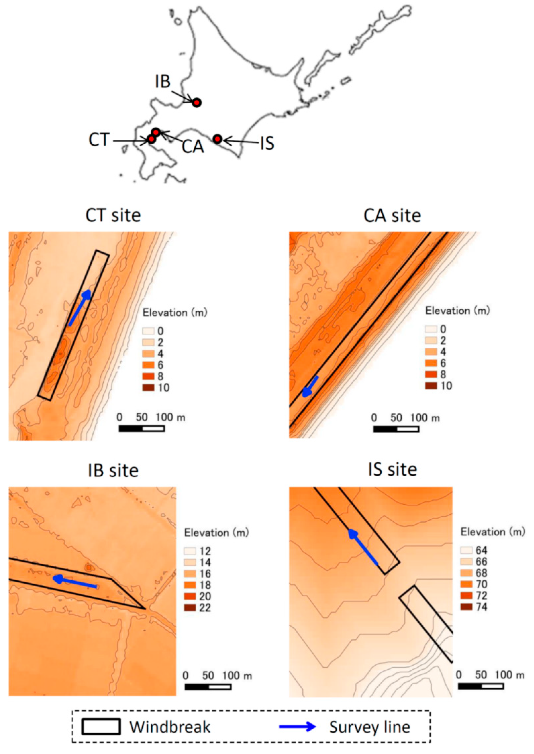
2.1. Study Site

The study was conducted at coastal and inland windbreaks at four sites in Hokkaido Prefecture, Japan: at coastal windbreaks at Toyono (CT site: 42°25′ N, 140°19′ E) and Asahihama (CA site: 42°32′ N, 140°24′ E) in Oshamambe Town, and at inland windbreaks at Bibai (IB site: 43°18′ N, 141°49′ E) and Shinhidaka (IS site: 42°24′ N, 142°27′ E). The locations and topography of the study sites are shown in Figure 1. According to the Japan Meteorological Agency (http://www.data.kishou.go.jp/), the mean annual temperature and precipitation for the past 10 years (from 2008 to 2017) were 7.6 °C and 1324 mm in Oshamambe, 7.4 °C and 1195 mm in Bibai, and 8.3 °C and 1001 mm in Shinhidaka, respectively.

At the CT site, Pinus thunbergii Parlat. stands had declined and grew sparsely on sand dunes. A line transect was set parallel to the shoreline. The distance from the shoreline to the transect was about 180 m. Tree age varied between 23 and 56 years. The mean height of P. thunbergii trees was 4 m. Some of the P. thunbergii trees on the lower area of the sand dune, which is adjacent to a marsh, were dead. Soils at the CT site are primarily sandy.

At the CA site, Quercus dentata Thunb. had been planted in 2005 after P. thunbergii stands had declined. The mean height of Q. dentata trees was 1.4 m. A line transect was set parallel to the shoreline and at a distance of about 70 m from the shoreline. Soil at the CA site was comprised of coastal sand and buried andosol. Masaka, et al. [36] noted that P. thunbergii at nearby sites had been damaged as a result of excess soil moisture caused by a less permeable andosol layer at coastal windbreaks near the CA site. They showed that the mean depth of the andosol layer was 24 cm, and the layer was generally 5–15 cm thick, with sporadic areas > 30 cm thick. The saturated hydraulic conductivity of the andosol layer was 10⁻⁵ cm s⁻¹, whereas that of the coastal sand ranged from 10⁻² to 10⁻³ cm s⁻¹ [36]. Iwasaki, et al. [22] used a CPMP to confirm the presence of increased soil water content at a depth of 20–50 cm at a coastal windbreak near the CA site.

At the IB site, a line transect was set within an inland windbreak of Betula platyphylla var. japonica (Miq.) Hara. Soil at the IB site was peat. B. platyphylla var. japonica were planted in 1956. The windbreak site was waterlogged in the spring season, in spite of an open ditch that exists around the windbreak. Many of the B. platyphylla var. japonica trees within the windbreak had died recently. Although the main cause of their decline was presumed to be an attack by the white-spotted longhorn beetle (Anoplophora malasiaca) (K. Masaka, unpublished data), the high groundwater level may also have contributed to their decline.

At the IS site, a line transect was set along the edge of an inland windbreak of Larix kaempferi (Lamb.) Carriere. The soil was andosol. Soil compaction may have occurred because the windbreak was planted adjacent to pasture, and heavy farm equipment sometimes passes near the edge of the windbreak. Tree age and the mean height of L. kaempferi in the windbreak were about 70 years and 28 m, respectively.

Table 1. Dates of the ground-penetrating radar (GPR) survey and combined penetrometer–moisture probe (CPMP) observations alongside antecedent precipitation data at each study site. The final column lists the associated date on which the volumetric soil water content (θ) was verified.

Site	GPR Survey and Simultaneous CPMP Observations			Verification Date
	Observation Date	Antecedent Precipitation (1 Day) (mm)	Antecedent Precipitation (1 Week) (mm)
CT	26 October 2015	0.5	34.5	23 October 2013 26 October 2015
CA	27 October 2015	0.0	28.0	27 October 2015
IB	7 June 2016	0.0	47.5	7 June 2016 8 May 2019
IS	20 October 2016	5.0	6.0	14 November 2018

lists the dates of the GPR survey and CPMP observations at each study site, as well as precipitation details prior to the observations. Antecedent precipitation was relatively low at all of the study sites. The depth of the andosol layer was investigated using a soil auger at the points where the CPMP observations were taken in the CA site. A topographic survey was conducted at the CT site, which is located on a sand dune and has a larger slope than the other sites (Figure 1).

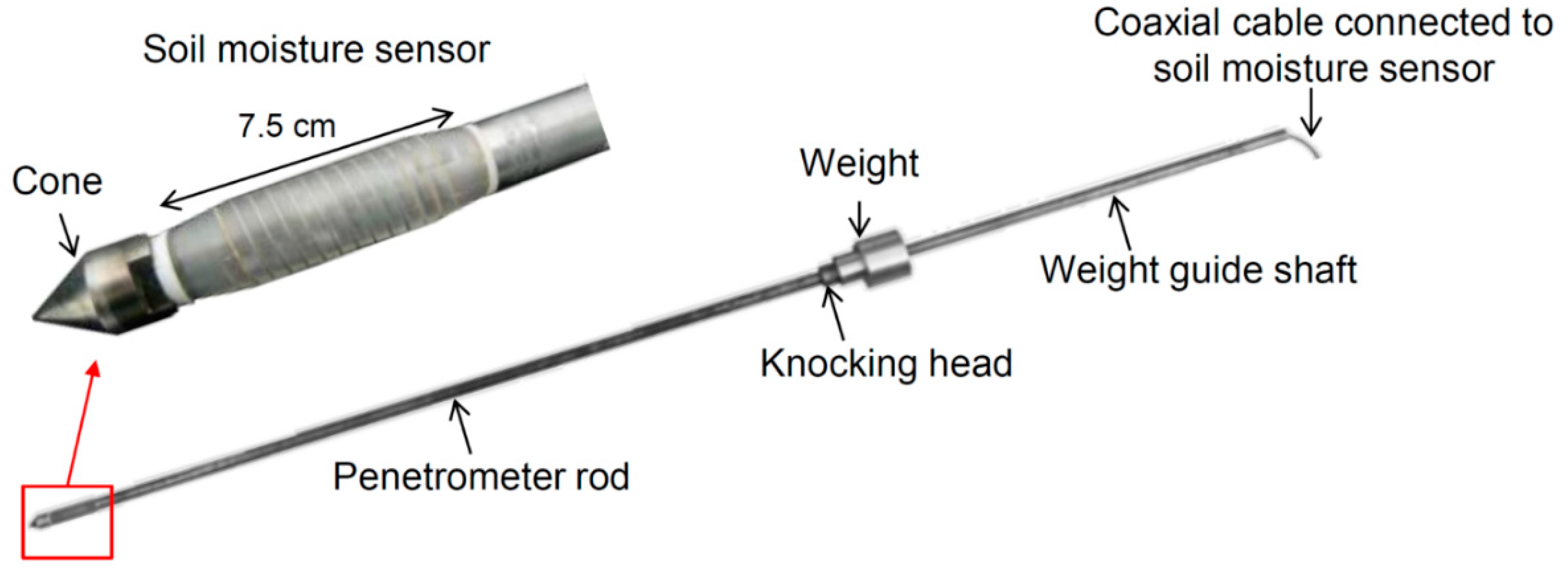
2.2. CPMP Observations

CPMP observations were conducted at several points along the line transect within two hours after the GPR survey was completed. Points with a characteristic GPR profile pattern were selected as observation points for the CPMP survey. The CPMP developed by Kosugi, et al. [18] was used in this study (Figure 2). The operation of the penetrometer involves a 2 kg weight free-falling 50 cm along a guide-shaft to strike a knocking-head that drives the cone (60° bit and 2.0 cm diameter) into the soil in the direction of gravity. The penetration resistance, N_C, is computed as the number of blows required to achieve 10 cm of penetration. A coil-type moisture probe is attached to a cone penetrometer. The TDR method is used to determine the volumetric soil water content, θ. The square root of the apparent dielectric constant, ξ (= κ^1/2), at each depth was measured using TDR 100 and PCTDR software (Campbell Scientific, Inc., Logan, UT, USA). The θ-ξ relationship developed for conventional rod-type TDR probes, e.g., [37] is commonly used to calculate θ. However, this relationship is not applicable to the coil-type TDR probe of the CPMP due to its S-shaped θ-ξ relation [18,38,39]. An empirical relationship calibrated to three soil types was, therefore, applied in the present study using the CPMP by Kosugi, et al. [18]:

$$\begin{gathered} \theta =\left(2.127491\times {10}^{-2}\right){\xi }^6-\left(3.897577\times {10}^{-1}\right){\xi }^5+\left(2.843453\right){\xi }^4-\left(10.47385\right){\xi }^3 \\ +\left(20.28508\right){\xi }^2-\left(19.04845\right)\xi +6.571050, \left(\theta \le 0.6901\right) \end{gathered}$$

(1)

The following equation was used if θ > 0.6901 because this value represents the maximum θ of the soil samples used to determine Equation (1) [18].

$$\theta =\left(0.4198\right)\xi -1.3321, (\theta >0.6901)$$

(2)

To eliminate variation between the moisture probes, the observed $\widehat{\xi }$ values of each probe were transformed into ξ values, which correspond to ξ′ measured by the reference probe to determine Equations (1) and (2) according to Kosugi, et al. [18]:

$$\xi =\frac{\left(\xi {\prime }_w-\xi {\prime }_a\right)}{\left({\widehat{\xi }}_w-{\widehat{\xi }}_a\right)}\left(\widehat{\xi }-{\widehat{\xi }}_a\right)+\xi {\prime }_a$$

(3)

where ${\widehat{\xi }}_w$ and ${\widehat{\xi }}_a$ represent observations in water and air by each probe, respectively, and $\xi {\prime }_w$ (=5.555) and $\xi {\prime }_a$ (=1.3568) represent observations in water and air by the reference probe. If $\xi$ > ${\widehat{\xi }}_w$, θ was assumed to be 1. Further details of the CPMP system are described by Kosugi, et al. [18] and Yamakawa, et al. [19].

In addition to the CPMP observations just after the GPR surveys, further CPMP observations were made and 100 cm³ soil cores were simultaneously sampled at several depths at a point on the line transect to verify θ measured by the CPMP. The θ value was then calculated by weighing the 100-cm³ soil sample before and after oven drying at 105 °C for 24–48 h in the laboratory. The θ verification dates at each study site are listed in Table 1. Although these dates differed from the dates of GPR surveys at some sites, the verification was to compare θ obtained by the gravimetric method with CPMP data collected on the same day and was not related to GPR survey dates.

To compare the CPMP observation results with those of GPR surveys, special points of N_C and θ were determined. Soil porosity, measured using a digital actual volumenometer (DIK-1150, Daiki Rika Kogyo Co. Ltd., Saitama, Japan), was between 0.41–0.46 (n = 2) at the CT site and 0.85–0.93 (n = 7) at the IB site. At the CT and IB sites, the shallowest depth of the soil layer with θ greater than the minimal porosity value (0.41 and 0.85, respectively) was regarded as the depth of the groundwater table. At the CA site, the shallowest and the deepest soil depths with increased θ values were plotted to determine the depth with excess soil moisture. At the IS site, the deepest depth with N_C > 30 was plotted to determine the depth affected by soil compaction.

2.3. GPR Surveys

The GPR data were collected using the pulseEKKO 1000A GPR system (Sensors and Software Inc., Mississauga, ON, Canada). The use of an antenna with a lower frequency allows for an increase in the penetration depth, but it decreases the spatial resolution because of the longer wavelength. In this study, a 900 MHz antenna was used to investigate the soil in detail within about a 100 cm depth, which is especially important for the growth base of windbreaks. The GPR data were collected every 10 cm along the same line transects as for the CPMP observations. Litter layers were not removed at any of the sites. Underbrush was cleared before the GPR survey at only the IB site to remove the thick growth of bamboo (Sasa senanensis).

The ξ measured by the CPMP is useful for estimating the spatial distribution of the radar wave velocity, V, because the magnetic permeability of soil is simplified in most cases to the free-space value [32]. At each CPMP observation point, V was calculated using the following equation in accordance with the method proposed by Yamakawa, et al. [19]:

$$V=c/\xi$$

(4)

where c is the velocity of light passing through a vacuum. A two-layer model of V has typically been used in previous studies conducted at sites with shallow groundwater because V differs significantly between saturated and unsaturated soil [25,26]. Therefore, the two-layer model was applied at the CT and IB sites because these sites had groundwater tables within a 100 cm depth. The boundary depth of the two layers was determined to minimize the root mean squared error between V in the model and V estimated from the CPMP data. At the CT site, V of 0.14 and 0.09 m ns⁻¹ was used for soil above and below a 320 cm elevation, respectively. At the IB site, a V of 0.09 and 0.06 m ns⁻¹ was used for soil above and below a 15 cm depth from the soil surface, respectively. At the CA and IS sites, the average calculated value of V (0.11 and 0.08 m ns⁻¹ at the CA and IS sites, respectively) was used for all depths because the spatial distribution of ξ fell within a narrow range.

The GPR data was processed and radargrams were drawn using RADPRO software (Korea Institute of Geoscience and Mineral Resources, Daejeon, Korea). The processing sequence and drawing parameters employed at all the study sites are summarized as follows:

• Dewow filtering.
• Gain correction using a linear function for the reflection time from 0 to 10 ns (1 dB at 0 ns and 30 dB at 10 ns) and a constant value of 30 dB for the reflection time longer than 10 ns.
• Filtering in wavenumber domain (minimum wavelength = 0.1 m, maximum wavelength = 10 m).
• Normal move out correction.
• Finite difference migration using V at each site (topography was also used at the CT site).
• Color table from white (minimum amplitude of −15 mV) to black (maximum amplitude of 15 mV).
• A horizontal drawing scale of 10 pixels m⁻¹, and a vertical drawing scale of 200 pixels m⁻¹.

The processing and drawing details using RADPRO are described in a user’s guide by Kim [40]. The reflecting interface (i.e., a continuous area with strong reflection in the radargram) was marked manually at the sites where it was clearly observed. In order to highlight the area with strong reflection, the area in which the median amplitude within a radius of five pixels was >15 mV in the radargrams was also drawn. Reflections with an amplitude of >15 mV were drawn as black pixels, and others were drawn as white pixels by setting the threshold amplitude of the radargram as 15 mV using RADPRO. Subsequently, median filtering (radius of five pixels) was carried out using ImageJ (NIH, Bethesda, MD, USA) [41].

3. Results

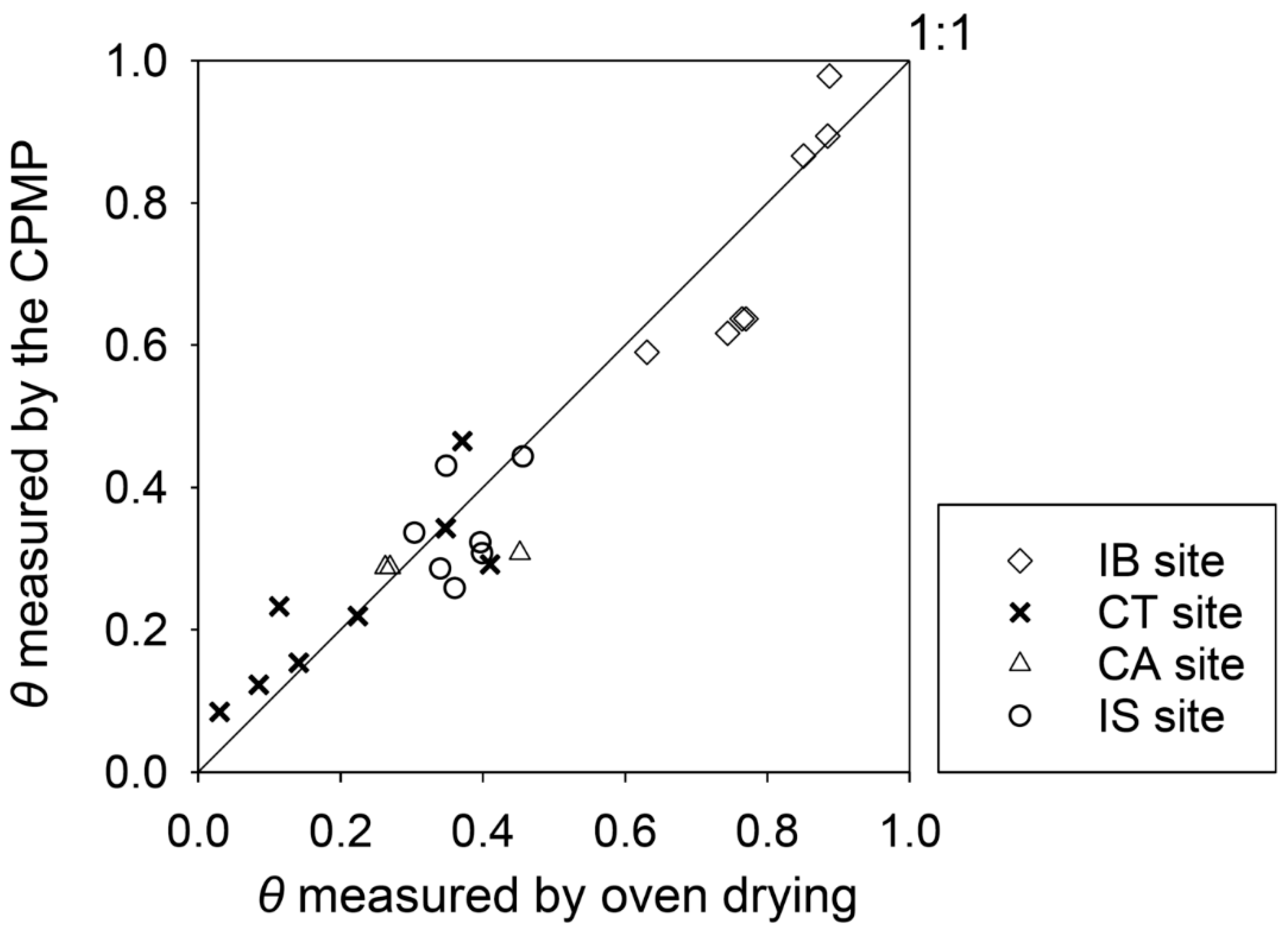
3.1. Comparison of θ Measured by the CPMP and the Gravimetric Method

The relationship between θ measured by the gravimetric method and θ measured by the CPMP is shown in Figure 3. At some sampling points, θ values measured by the two methods differed from each other by about 0.1. However, the relationship between the two values did not deviate considerably from the 1:1 line at any study site, and the size of the measurement error by the CPMP did not change with respect to the soil type.

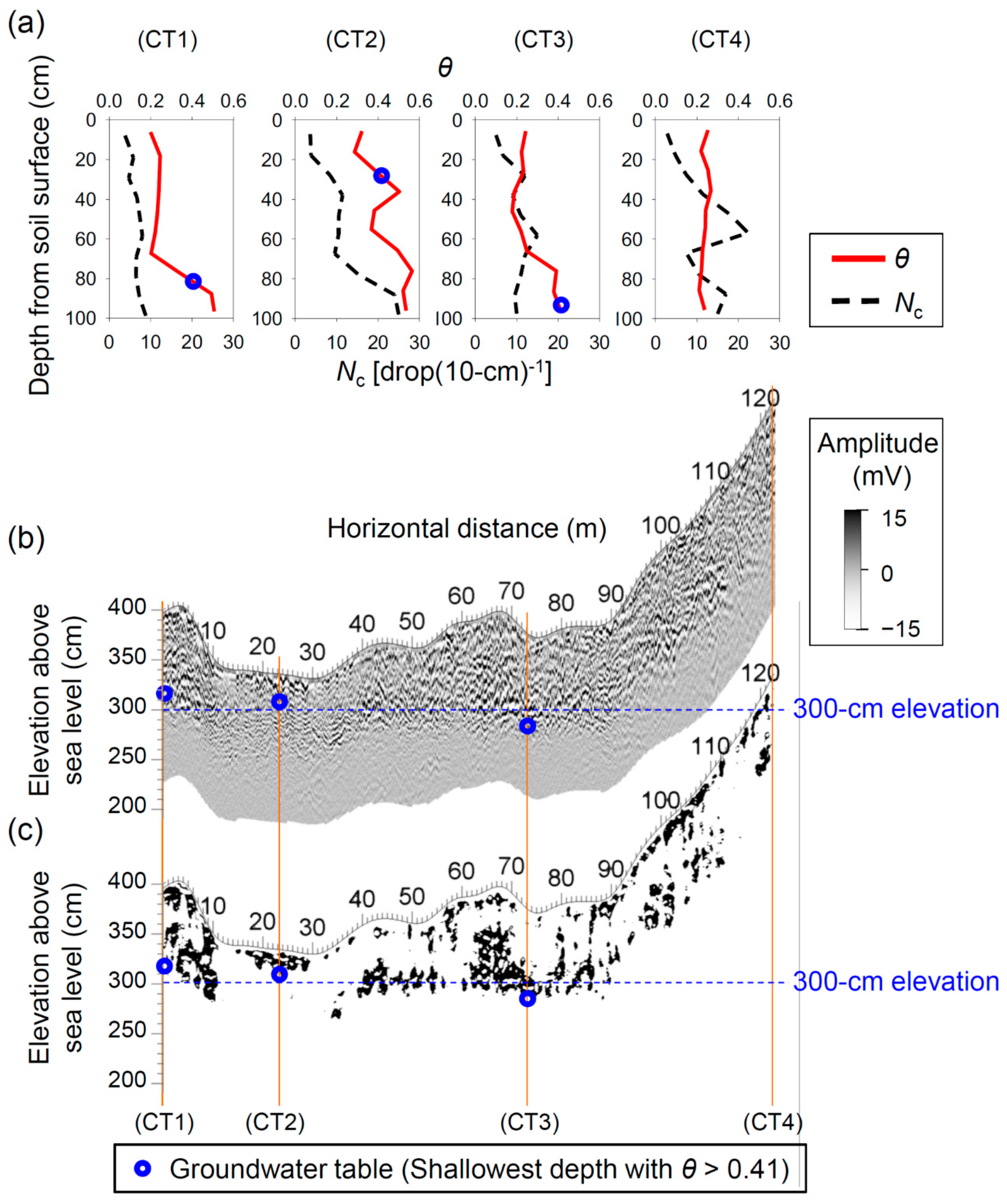
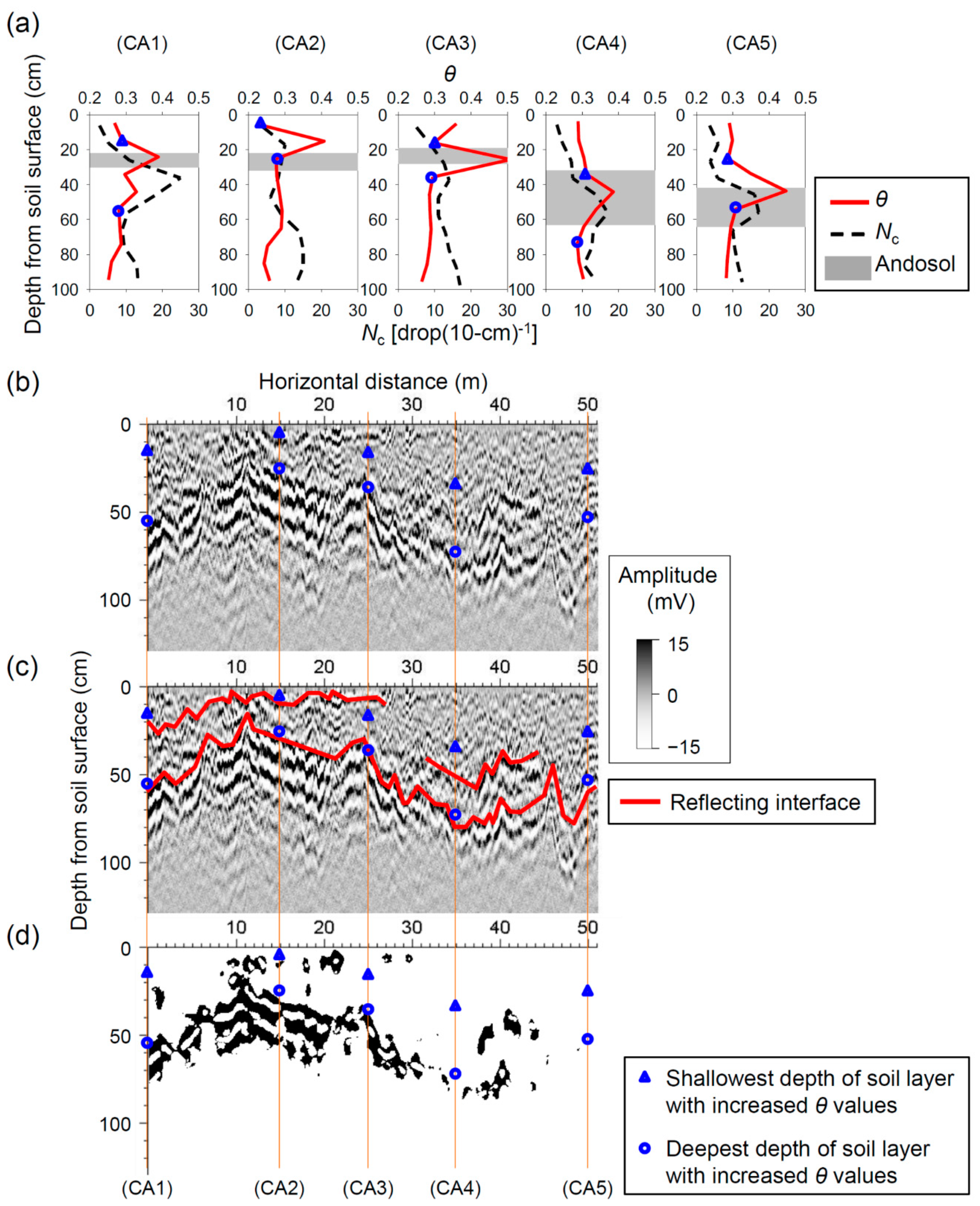
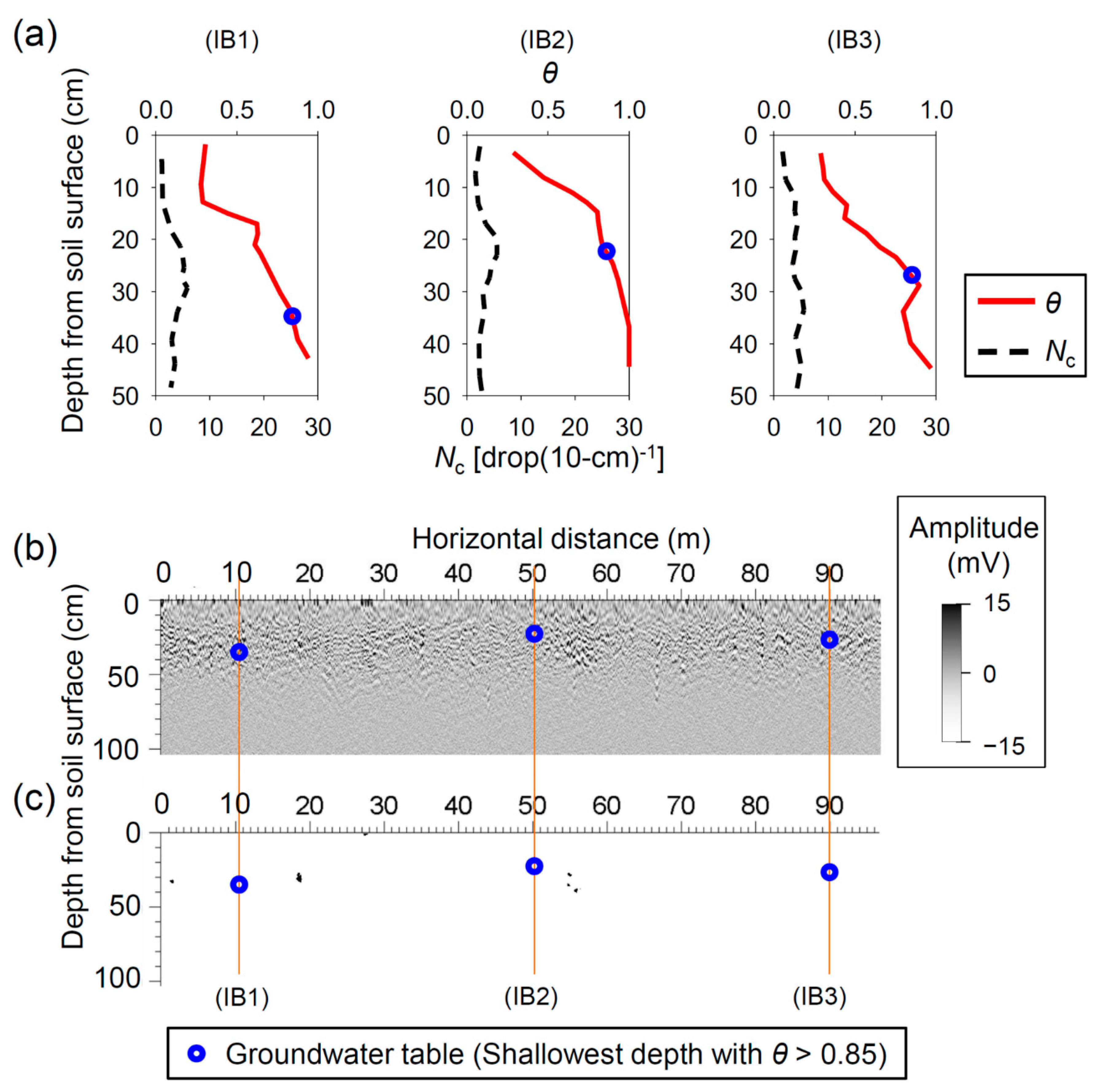
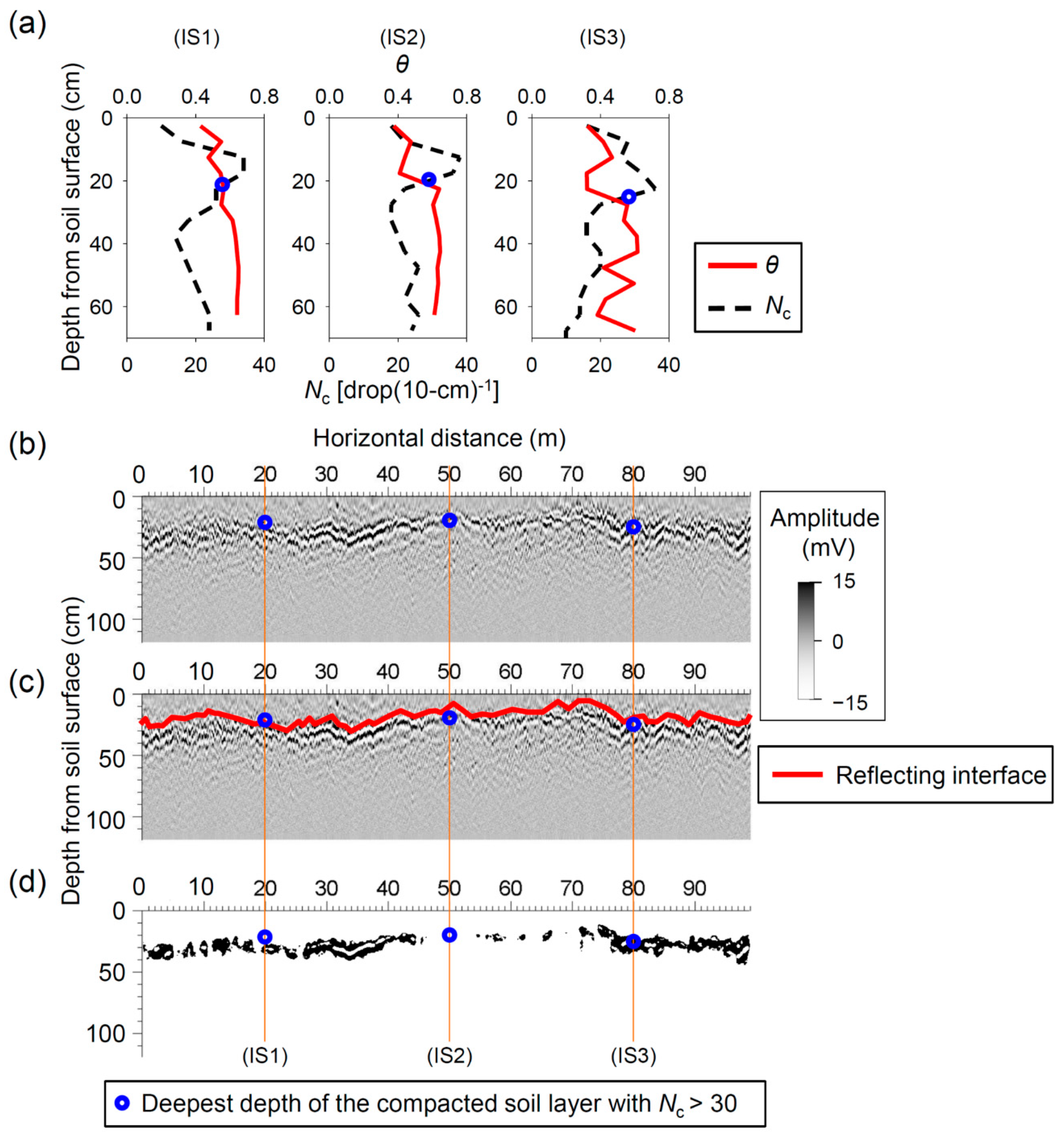
3.2. Profiles of GPR Reflection and CPMP Measurements

At the CT site, the vertical profile of θ measured by the CPMP varied depending on the elevation (Figure 4a): θ was approximately 0.2 at a depth of 0–60 cm and increased in depth from 70 cm to 90 cm at CT1 and CT3, whereas it was greater than 0.41 at nearly all depths > 30 cm at CT2. At CT4, the groundwater table was not observed at less than a 100-cm depth. The groundwater table was plotted at an elevation of 280–320 cm at CT1, CT2, and CT3 (Figure 4b). As for the radargram, the attenuation depth was different among locations, although the reflecting interface seemed to be obscured at this site (Figure 4b). Where the horizontal distance was greater than 90 m, GPR reflection was attenuated below a depth of about 100 cm from the soil surface (Figure 4b,c). This suggests that the maximal depth of GPR penetration with the 900 MHz antenna was about 100 cm in this site. In contrast, in the region with a horizontal distance of 0–90 m, the attenuation depth of GPR reflection varied among locations, resulting in the attenuation at an elevation of 280–320 cm, which corresponded well to the groundwater level detected by the CPMP observation (Figure 4b,c). The GPR and CPMP results indicate that the groundwater table was at an elevation of 280–320 cm and that the groundwater level from the soil surface was shallow at the lower part of the sand dune.

At the CA site, the soil auger was able to detect the andosol layer at a depth of 20–30 cm from CA1, CA2, and CA3, and at a depth of 30–70 cm at CA4 and CA5 (Figure 5a). At each point, the highest θ was observed using the CPMP at or just above the depth with high N_C near the andosol layer at each point (Figure 5a). These results agree with previous studies that found the less permeable buried andosol layer caused excess soil moisture at coastal windbreaks near the CA site [36]. At CA1, the soil had higher θ and N_C at the 40 cm depth than at depths of 50–100 cm, although this soil was below an andosol layer (Figure 5a). This was attributable to the existence of a compacted sand layer at around a 40-cm depth, which was confirmed by a survey using the soil auger. As for the radargram, a continuous reflecting interface was detected at a 20–80 cm depth at all horizontal distances, with another reflecting interface above it at the horizontal distances of 0–27 m and 32–44 m (Figure 5b,c). The deeper reflecting interface could be detected more clearly than the shallower reflecting interface (Figure 5b–d). The deeper reflecting interface corresponded well to the deepest depth of the soil layer with increased θ values at all distances of the survey line (Figure 5c). Moreover, the depth of the shallower reflecting interface was similar to the shallowest depth of the soil layer with increased θ values at many distances, although it was unclear at some distances, such as CA5 (Figure 5c). These findings suggest that the location of the soil layer with increased θ values is between shallower and deeper reflecting interfaces. Thus, GPR facilitated interpolation of the spatial distribution of the soil layer with excess soil moisture between the CPMP survey points. For instance, it should exist at 0–20 cm and 40–70 cm depths at the horizontal distances of 10 and 40 m, respectively (Figure 5c).

At the IB site, θ was nearly 1.0 at a 40–50 cm depth, and the groundwater table depth estimated using the CPMP was shallower at IB2 than at both IB1 and IB3 (Figure 6a). However, GPR could not identify the differences in θ between these points because the reflection was attenuated from the soil surface at all distances along the survey line (Figure 6b,c). This indicates that GPR was not suitable for determining the depth of the groundwater table at the IB site.

At the IS site, the CPMP identified the compaction of the soil layer at some depths between 10 and 30 cm (Figure 7a). θ was 0.3–0.5 at the depth of the soil compaction and was greater than 0.6 below the compaction depth (Figure 7a). GPR could detect the reflecting interface within a 10–30 cm depth (Figure 7b–d). The reflecting interface was similar to the deepest depth of the compacted soil layer (Figure 7c). The radargram indicates that the deepest depth of the compacted soil layer was spatially homogeneous and approximately 20 cm throughout the survey line.

4. Discussion

4.1. Applicability of a CPMP in Windbreaks

Using a CPMP to estimate the soil water content was applicable regardless of the soil type. Rigorous calibration for the relationship between ξ and θ in each site may improve the accuracy of θ measurements. However, the CPMP data did not show any sizable errors in estimating θ using Equations (1)–(3) at any of the sites with different soil types (Figure 3). The usefulness of these equations was also validated for sandy and loamy layers [18] and a volcanic ash layer [21]. Thus, Equations (1)–(3) are sufficient for evaluating the soil moisture condition in windbreaks.

4.2. Applicability of GPR in Windbreaks

GPR could detect the soil layer affected by compaction or less permeable layers at many distances of the survey line (Figure 5 and Figure 7). In our study sites, θ changed clearly at depths where compaction occurred or where less permeable layers existed (Figure 5 and Figure 7). As vertical contrasts in θ can produce strong GPR reflections in shallow soils [42,43], the reflecting interface corresponded to the soil depth with a large vertical contrast in θ. The reflecting interface caused by soil compaction was also reported in previous studies using GPR in agricultural fields [28,29,44]. Thus, GPR should be suitable for evaluating the spatial distribution of less permeable layers and soil layers affected by compaction at coastal and inland windbreaks.

On the other hand, an obscure or no reflecting interface was observed at the depth of the groundwater table in coastal and inland windbreaks (Figure 4 and Figure 6). One possible reason for that is the gradual increase in θ with depth at the transition zone above the groundwater table (Figure 4a and Figure 6a) because reflections from the groundwater table will not be observed when the dominant wavelength of GPR is short compared with the thickness of the transition zone [45]. Although the reflecting interface was obscure, the spatial distribution of the groundwater table could be evaluated from examining the attenuation of the GPR reflection at the CT site (Figure 4b,c). The attenuation of the GPR reflection increases with increasing electrical conductivity of the material (σ) [32]. As the soil σ increases with increasing θ [31,32], high θ beneath the groundwater table can cause a large attenuation of the GPR reflection. Sea salt in groundwater may have also contributed to the high σ and large GPR reflection attenuation. In a coastal windbreak with shallow groundwater, Kudou, et al. [30] found that the attenuation depth of the GPR reflection estimated from the binarization of the radargram with a 900-MHz antenna was useful for characterizing the area where the vigor of P. thunbergii trees had declined. Our results also suggest that the attenuation depth of GPR reflection is a useful indicator of the soil moisture condition in coastal windbreaks with shallow groundwater. In contrast to the CT site, the soil moisture condition could not be evaluated at the IB site because the GPR reflection was attenuated across the entire soil layer (Figure 6b,c). One possible reason for that is the high θ of nearly 1.0 at a depth shallower than 50 cm due to the large porosity of peat and the shallow groundwater level (Figure 6a). Though not removing leaf litter may also affect the GPR results, as leaf litter weakens the radargram contrast [46], it should not be the principal reason for the large attenuation at the IB site, as leaf litter was also not removed from the other study sites. Using a low-frequency antenna can reduce the attenuation of the GPR reflection [32]. Furthermore, as demonstrated by Harari [47] and Bano [45], a longer wavelength of the low-frequency antenna may produce a clearer reflecting interface at the groundwater table depth. However, as a low-frequency antenna has low vertical spatial resolution [32], it is not suitable for identifying shallow groundwater tables. Therefore, GPR should not be suitable for peat with groundwater levels shallower than 50 cm.

4.3. Combined Use of a CPMP and GPR to Evaluate Soil Moisture and Soil Hardness in Windbreaks

Ground truth data of the GPR profile were obtained by drilling boreholes [26,34] or installing wells [35] in studies for detecting the groundwater table. In GPR studies for detecting soil compaction, ground truth data were obtained using a penetrometer [28,44] or by collecting soil samples [48]. These conventional methods require significant effort and must evaluate groundwater level and soil hardness separately. Our results show that the CPMP was useful for detecting the groundwater table, less permeable layers, and soil compaction (Figure 4, Figure 5, Figure 6 and Figure 7). Thus, a CPMP can provide ground truth data for GPR more effectively compared to the conventional methods. Meanwhile, GPR was useful for interpolating the information between the survey points made with the CPMP because GPR can provide horizontally continuous images. Therefore, the combination of GPR and a CPMP was effective for evaluating the spatial distribution of soil hardness and soil moisture with a vertically and horizontally high spatial resolution.

As there was only one case study using GPR [30] or a CPMP [22] to measure soil moisture and soil hardness in windbreaks, we examined the application limitations of these two methods. Our findings indicate that GPR was unsuitable for soil with θ close to 1.0 at a depth shallower than 50 cm. Previous studies have reported that GPR was also unsuitable for soil with high electrical conductivity [31] or an interlayering of loam and gravel [19]. The CPMP was applicable regardless of the soil type; therefore, we recommend that CPMP observations be conducted first, followed by a GPR survey if the site has the soil characteristics suitable for a GPR survey and there is a need to interpolate the information between the survey points.

5. Conclusions

The combination of GPR and a CPMP was useful for evaluating the spatial distribution of the less permeable layer and the groundwater table in coastal windbreaks and the soil layer affected by soil compaction in an inland windbreak underlain with andosol soils. As the applicability of GPR was limited in an inland windbreak with peat, GPR surveys should not be conducted at windbreaks with high soil water content near the soil surface. The CPMP was useful for interpreting the GPR profiles, and GPR was useful for interpolating the information between the survey points of CPMP. Therefore, the combination of GPR and a CPMP should be more effective than using either GPR or a CPMP alone for investigating the spatial distribution of soil moisture and soil hardness at windbreaks, as long as the sites have the soils to which both methods are applicable. The combined use of GPR with a CPMP will help reduce windbreak management costs by easily identifying areas with high soil moisture or hard soil.

References

1. Zhu, J.J.; Gonda, Y.; Matsuzaki, T.; Yamamoto, M. Salt distribution in response to optical stratification porosity and relative windspeed in a coastal forest in Niigata, Japan. Agrofor. Syst. 2002, 56, 73–85. [Google Scholar] [CrossRef]
2. Kathiresan, K.; Rajendran, N. Coastal mangrove forests mitigated tsunami. Estuar. Coast. Shelf Sci. 2005, 65, 601–606. [Google Scholar] [CrossRef]
3. Torita, H.; Tanaka, N.; Masaka, K.; Iwasaki, K. Effects of forest management on resistance against tsunamis in coastal forests. Ocean Eng. 2018, 169, 379–387. [Google Scholar] [CrossRef]
4. Kort, J. Benefits of windbreaks to field and forage crops. Agric. Ecosyst. Environ. 1988, 22–23, 165–190. [Google Scholar] [CrossRef]
5. Iwasaki, K.; Torita, H.; Abe, T.; Uraike, T.; Touze, M.; Fukuchi, M.; Sato, H.; Iijima, T.; Imaoka, K.; Igawa, H. Spatial pattern of windbreak effects on maize growth evaluated by an unmanned aerial vehicle in Hokkaido, northern Japan. Agrofor. Syst. 2019, 93, 1133–1145. [Google Scholar] [CrossRef]
6. Song, L.; Zhu, J.; Yan, Q.; Li, M.; Yu, G. Comparison of intrinsic water use efficiency between different aged Pinus sylvestris var. mongolica wide windbreaks in semiarid sandy land of northern China. Agrofor. Syst. 2015, 89, 477–489. [Google Scholar] [CrossRef]
7. Antonellini, M.; Mollema, P.N. Impact of groundwater salinity on vegetation species richness in the coastal pine forests and wetlands of Ravenna, Italy. Ecol. Eng. 2010, 36, 1201–1211. [Google Scholar] [CrossRef]
8. Oda, T. Study on the reaction of planted tree root systems to water-logging and its application to developing forests in damp lowlands of coastal sand dunes. Spec. Bull. Chiba Pref. For. Res. Center 2001, 3, 1–78. (In Japanese) [Google Scholar]
9. Fukuchi, M.; Torita, H. The growth and survival of shelterbelts of Norway spruce (Picea abies) in central Hokkaido. Trans. Meet. Hokkaido Branch Jpn. For. Soc. 1996, 44, 17–19. (In Japanese) [Google Scholar]
10. Hirano, Y.; Todo, C.; Yamase, K.; Tanikawa, T.; Dannoura, M.; Ohashi, M.; Doi, R.; Wada, R.; Ikeno, H. Quantification of the contrasting root systems of Pinus thunbergii in soils with different groundwater levels in a coastal forest in Japan. Plant Soil 2018, 426, 327–337. [Google Scholar] [CrossRef]
11. Todo, C.; Tokoro, C.; Yamase, K.; Tanikawa, T.; Ohashi, M.; Ikeno, H.; Dannoura, M.; Miyatani, K.; Doi, R.; Hirano, Y. Stability of Pinus thunbergii between two contrasting stands at differing distances from the coastline. For. Ecol. Manag. 2019, 431, 44–53. [Google Scholar] [CrossRef]
12. Shinomiya, Y.; Imaya, A.; Takanashi, K.; Sakamoto, T. The physical property of embankment with a rain pool: A case study of embankment built in the early stage of the Coastal Forest Restoration Project after tsunami. Bull. FFPRI 2016, 15, 151–159. (In Japanese) [Google Scholar]
13. Ono, K.; Komoriya, A.; Tachibana, R.; Imaya, A.; Suzuki, S.; Noguchi, H.; Noguchi, K.; Hagino, H. Effects of row deep tillage for the growth base formed by piling up soil in damp lowlands behind coastal sand dunes to construct coastal disaster prevention forest belts on the Kujukuri coastline, Japan. Soil Sci. Plant Nutr. 2018, 64, 168–180. [Google Scholar] [CrossRef]
14. Vaz, C.M.P.; Hopmans, J.W. Simultaneous measurement of soil penetration resistance and water content with a combined penetrometer–TDR moisture probe. Soil Sci. Soc. Am. J. 2001, 65, 4–12. [Google Scholar] [CrossRef] [Green Version]
15. Topp, G.; Lapen, D.; Edwards, M.; Young, G. Laboratory calibration, in-field validation and use of a soil penetrometer measuring cone resistance and water content. Vadose Zone J. 2003, 2, 633–641. [Google Scholar] [CrossRef]
16. Sun, Y.; Schulze Lammers, P.; Ma, D. Evaluation of a combined penetrometer for simultaneous measurement of penetration resistance and soil water content. J. Plant Nutr. Soil Sci. 2004, 167, 745–751. [Google Scholar] [CrossRef]
17. Lin, C.P.; Tang, S.H.; Chung, C.C. Development of TDR penetrometer through theoretical and laboratory investigations: 1. Measurement of soil dielectric permittivity. Geotech. Test. J. 2006, 29, 306–313. [Google Scholar] [CrossRef]
18. Kosugi, K.; Yamakawa, Y.; Masaoka, N.; Mizuyama, T. A combined penetrometer–moisture probe for surveying soil properties of natural hillslopes. Vadose Zone J. 2009, 8, 52–63. [Google Scholar] [CrossRef]
19. Yamakawa, Y.; Kosugi, K.; Masaoka, N.; Tada, Y.; Mizuyama, T. Use of a combined penetrometer-moisture probe together with geophysical methods to survey hydrological properties of a natural slope. Vadose Zone J. 2010, 9, 768–779. [Google Scholar] [CrossRef]
20. Masaoka, N.; Kosugi, K.; Yamakawa, Y.; Mizuyama, T.; Tsutsumi, D. Application of a combined penetrometer-moisture probe for investigating heterogeneous hydrological properties of a footslope area. Vadose Zone J. 2012, 11. [Google Scholar] [CrossRef]
21. Yamakawa, Y.; Hotta, N.; Tsunetaka, H.; Ohsaka, O.; Masaoka, N.; Imaizumi, F.; Kosugi, K. Investigation of volcanic deposits using a combined penetrometer-moisture probe: Application in Izu-Oshima Volcano, Japan. Int. J. Eros. Control Eng. 2018, 11, 15–27. [Google Scholar] [CrossRef] [Green Version]
22. Iwasaki, K.; Sato, H.; Masaka, K.; Torita, H.; Yamakawa, Y.; Kosugi, K. Use of a combined penetrometer-moisture probe for evaluating planting base of a coastal forest—A case study of Oshamambe, Hokkaido Prefecture. J. Jpn. Soc. Coast. For. 2016, 15, 39–43. (In Japanese) [Google Scholar]
23. Hasegawa, S.; Tabata, M.; Kozawa, T.; Sato, Y. Relationship between physicality of soil and tree vigour in planting area maked by heavy construction machine—An example of high way planting area. J. Jpn. Inst. Landsc. Archit. 1984, 48, 104–122. (In Japanese) [Google Scholar] [CrossRef] [Green Version]
24. Sato, H.; Tsuda, T.; Kuramoto, S.; Iida, S.; Hashimoto, T. Recovery of soil penetration resistance on compacted skid trails after forest thinning in central Hokkaido. J. Jpn. For. Soc. 2018, 100, 110–115. (In Japanese) [Google Scholar] [CrossRef]
25. Bristow, C.S.; Pucillo, K. Quantifying rates of coastal progradation from sediment volume using GPR and OSL: The Holocene fill of Guichen Bay, south-east South Australia. Sedimentology 2006, 53, 769–788. [Google Scholar] [CrossRef]
26. Igel, J.; Günther, T.; Kuntzer, M. Ground-penetrating radar insight into a coastal aquifer: The freshwater lens of Borkum Island. Hydrol. Earth Syst. Sci. 2013, 17, 519–531. [Google Scholar] [CrossRef] [Green Version]
27. Gómez-Ortiz, D.; Martín-Crespo, T.; Rodríguez, I.; Sánchez, M.; Montoya, I. The internal structure of modern barchan dunes of the Ebro River Delta (Spain) from ground penetrating radar. J. Appl. Geophys. 2009, 68, 159–170. [Google Scholar] [CrossRef]
28. Raper, R.L.; Asmussen, L.E.; Powell, J.B. Sensing hard pan depth with ground penetrating radar. Trans. ASAE 1990, 33, 41–46. [Google Scholar] [CrossRef]
29. André, F.; Leeuwen, C.v.; Saussez, S.; Durmen, R.V.; Bogaert, P.; Moghadas, D.; Rességuier, L.d.; Delvaux, B.; Vereecken, H.; Lambot, S. High-resolution imaging of a vineyard in south of France using ground-penetrating radar, electromagnetic induction and electrical resistivity tomography. J. Appl. Geophys. 2012, 78, 113–122. [Google Scholar] [CrossRef]
30. Kudou, K.; Nishikawa, H.; Fujii, H.; Asaka, T. Study on the interpretation of subsurface water environment to affect a growth condition of the shore forest using the property of electromagnetic reflectance property. J. Jpn. Soc. Civil Eng. Ser. G 2008, 64, 96–106. (In Japanese) [Google Scholar] [CrossRef]
31. Doolittle, J.A.; Minzenmayer, F.E.; Waltman, S.W.; Benham, E.C.; Tuttle, J.W.; Peaslee, S.D. Ground-penetrating radar soil suitability map of the conterminous United States. Geoderma 2007, 141, 416–421. [Google Scholar] [CrossRef]
32. Jol, H.M. Ground Penetrating Radar: Theory and Applications; Elsevier: Amsterdam, The Netherlands, 2009; p. 545. [Google Scholar]
33. Lorenzo, H.; Pérez-Gracia, V.; Novo, A.; Armesto, J. Forestry applications of ground-penetrating radar. For. Syst. 2014, 19, 5–17. [Google Scholar] [CrossRef] [Green Version]
34. Rejiba, F.; Bobée, C.; Maugis, P.; Camerlynck, C. GPR imaging of a sand dune aquifer: A case study in the niayes ecoregion of Tanma, Senegal. J. Appl. Geophys. 2012, 81, 16–20. [Google Scholar] [CrossRef]
35. Doolittle, J.A.; Jenkinson, B.; Hopkins, D.; Ulmer, M.; Tuttle, W. Hydropedological investigations with ground-penetrating radar (GPR): Estimating water-table depths and local ground-water flow pattern in areas of coarse-textured soils. Geoderma 2006, 131, 317–329. [Google Scholar] [CrossRef]
36. Masaka, K.; Torita, H.; Sato, H.; Kon, H.; Sato, H.; Fukuchi, M. Decline of Pinus thunbergii Parlat. stands due to excess soil moisture caused by a buried andosol layer at a coastal sand site in Hokkaido, northern Japan. J. For. Res. 2010, 15, 341–346. [Google Scholar] [CrossRef]
37. Topp, G.C.; Davis, J.L.; Annan, A.P. Electromagnetic determination of soil water content: Measurements in coaxial transmission lines. Water Resour. Res. 1980, 16, 574–582. [Google Scholar] [CrossRef] [Green Version]
38. Subedi, S.; Kawamoto, K.; Karunarathna, A.K.; Moldrup, P.; Wollesen de Jonge, L.; Komatsu, T. Mini tensiometer-time domain reflectometry coil probe for measuring soil water retention properties. Soil Sci. Soc. Am. J. 2013, 77, 1517–1528. [Google Scholar] [CrossRef]
39. Katsura, S.; Kosugi, K.; Mizuyama, T. Application of a coil-type TDR probe for measuring the volumetric water content in weathered granitic bedrock. Hydrol. Process. 2008, 22, 750–763. [Google Scholar] [CrossRef]
40. Kim, J.H. RADPRO V.3.4 User’s Guide; KIGAM: Daejeon, Korea, 2004; p. 84. [Google Scholar]
41. Schneider, C.A.; Rasband, W.S.; Eliceiri, K.W. NIH Image to ImageJ: 25 years of image analysis. Nat. Methods 2012, 9, 671–675. [Google Scholar] [CrossRef]
42. Kowalsky, M.B.; Dietrich, P.; Teutsch, G.; Rubin, Y. Forward modeling of ground-penetrating radar data using digitized outcrop images and multiple scenarios of water saturation. Water Resour. Res. 2001, 37, 1615–1625. [Google Scholar] [CrossRef] [Green Version]
43. Lunt, I.A.; Hubbard, S.S.; Rubin, Y. Soil moisture content estimation using ground-penetrating radar reflection data. J. Hydrol. 2005, 307, 254–269. [Google Scholar] [CrossRef]
44. Jonard, F.; Mahmoudzadeh, M.; Roisin, C.; Weihermüller, L.; André, F.; Minet, J.; Vereecken, H.; Lambot, S. Characterization of tillage effects on the spatial variation of soil properties using ground-penetrating radar and electromagnetic induction. Geoderma 2013, 207–208, 310–322. [Google Scholar] [CrossRef]
45. Bano, M. Effects of the transition zone above a water table on the reflection of GPR waves. Geophys. Res. Lett. 2006, 33, 1–5. [Google Scholar] [CrossRef] [Green Version]
46. Tanikawa, T.; Ikeno, H.; Dannoura, M.; Yamase, K.; Aono, K.; Hirano, Y. Leaf litter thickness, but not plant species, can affect root detection by ground penetrating radar. Plant Soil 2016, 408, 271–283. [Google Scholar] [CrossRef]
47. Harari, Z. Ground-penetrating radar (GPR) for imaging stratigraphic features and groundwater in sand dunes. J. Appl. Geophys. 1996, 36, 43–52. [Google Scholar] [CrossRef]
48. Wang, P.; Hu, Z.; Zhao, Y.; Li, X. Experimental study of soil compaction effects on GPR signals. J. Appl. Geophys. 2016, 126, 128–137. [Google Scholar] [CrossRef]
Figure 1. Locations and topography of study sites. Interval of contours is 1 m. Topographic data are based on 5-m (CT, CA, and IB sites) or 10-m (IS site) digital elevation models of the Geospatial Information Authority of Japan.
Geosciences 10 00238 g001
Figure 2. Photograph of the combined penetrometer–moisture probe (CPMP).
Geosciences 10 00238 g002
Figure 3. Relationship between θ measured by oven-drying a 100-cm3 soil core sample and θ measured by the CPMP for soils at different study sites.
Geosciences 10 00238 g003
Figure 4. (a) Vertical profiles of θ and NC measured by the CPMP, (b) radargram, and (c) the area in which the median amplitude within a radius of five pixels was > 15 mV in the radargram at the CT site.
Geosciences 10 00238 g004
Figure 5. (a) Vertical profiles of θ and NC measured by the CPMP, (b) radargram, (c) radargram with interpretation of the reflecting interface, and (d) the area in which the median amplitude within a radius of five pixels was > 15 mV in the radargram at the CA site.
Geosciences 10 00238 g005
Figure 6. (a) Vertical profiles of θ and NC measured by the CPMP, (b) radargram, and (c) the area in which the median amplitude within a radius of five pixels was > 15 mV in the radargram at the IB site.
Geosciences 10 00238 g006
Figure 7. (a) Vertical profiles of θ and NC measured by the CPMP, (b) radargram, (c) radargram with interpretation of the reflecting interface, and (d) the area in which the median amplitude within a radius of five pixels was > 15 mV in the radargram at the IS site.
Geosciences 10 00238 g007