Article

Long-Lasting Patterns in 3 kHz Electromagnetic Time Series after the ML = 6.6 Earthquake of 2018-10-25 near Zakynthos, Greece

by
Dimitrios Nikolopoulos
1,*,
Ermioni Petraki
2,
Panayiotis H. Yannakopoulos
2,
Georgios Priniotakis
1,
Ioannis Voyiatzis
2 and
Demetrios Cantzos
1
1
Department of Industrial Design and Production Engineering, University of West Attica, Petrou Ralli & Thivon 250, GR-12244 Aigaleo, Greece
2
Department of Informatics and Computer Engineering, University of West Attica, Agiou Spyridonos, GR-12243 Aigaleo, Greece
*
Author to whom correspondence should be addressed.
Geosciences 2020, 10(6), 235; https://doi.org/10.3390/geosciences10060235
Submission received: 10 April 2020 / Revised: 6 May 2020 / Accepted: 13 May 2020 / Published: 18 June 2020
(This article belongs to the Special Issue Electromagnetic and Radon Pre-earthquake Precursors)

Abstract

:
This paper reports one-month 3 kHz EM disturbances recorded at Kardamas, Ilia, Greece after a strong M L = 6.6 earthquake occurred on 2018/10/25 near Zakynthos and Ilia. During this period 17 earthquakes occurred with magnitudes M L = 4.5 and M L = 5.5 and depths between 3 km and 17 km, all near Zakynthos and Ilia. A two-stage, fully computational methodology was applied to the outcomes of five different time-evolving chaos analysis techniques (DFA, fractal dimension analysis through Higuchi, Katz and Sevcik methods and power-law analysis). Via literature-based thresholds, the out-of-threshold results of all chaos analysis methods were located and from these, the common time instances of 13 selected combinations per five, four, three and two methods. Numerous persistent segments were located with DFA exponents between 1.6 α 2.0 , fractal dimensions between 1.4 D 2.0 and power-law exponents between 2.2 β 3.0 . Out of the 17 earthquakes, six earthquakes were jointly matched by 13 selected combinations of five, four, three and two chaos analysis methods, four earthquakes by all combinations of four, three and two, while the remaining seven earthquakes were matched by at least one combination of three methods. All meta-analysis matches are within typical forecast periods.
PACS:
05.45.Gg; 91.25.-r; 91.25.Qi; 91.30.-f; 91.30.P-; 91.30.pa; 91.45.-c

Graphical Abstract

Research Highlights

  • One-month 3 kHz EM disturbances after the 2018/10/25, M L = 6.6 earthquake near Zakynthos Island and Ilia, Greece.
  • Computational recording of common dates with out-of-threshold results from five different chaos analysis techniques.
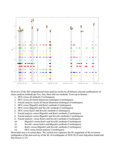
  • All 17 subsequent earthquakes were jointly matched by selected combinations of five, four, three and two chaos analysis methods.

1. Introduction

Earthquakes are natural phenomena that negatively impact society. Strong earthquakes are a major concern because they are destructive and occur inevitably when certain geophysical conditions are met, e.g., [1,2,3,4]. Seismic prognosis is significant among the scientific community but, despite the tremendous efforts, the earthquakes are still hard to predict [5,6,7,8]. Due to this, it remains an elusive and challenging task to identify credible and unambiguous seismic precursors [9]. To this end, different types of pre-earthquake signals are recorded [5,7,8,10,11], related to unusual activity in the regions of crust cracking and fracture [12]. There are two main ways to observe seismic precursors [7]: (a) Direct recording of electromagnetic disturbances originating from the earth’s crust as the materials at the center of earthquakes, under tectonic stress, emit naturally electromagnetic waves of various frequencies; (b) Indirect observation of propagation anomalies due to existing signals, since different types of anomalies that occur in the ionosphere and atmosphere prior to earthquakes can evoke anomalous propagation of emitted signals [7]. Both direct and indirect pre-seismic phenomena help to identify seismic sources.
In terms of earthquake prediction, five phases are usually recognized. First, is the establishment phase during which potential magnitudes and prediction time intervals of ensuing earthquakes are depicted in prediction maps. The remaining phases are subsequently divided as [7,10]: (A) long-term prediction (0–10 years); (B) intermediate prediction (0–1 year); (C) short-term prediction (3–36 days); (D) immediate prediction (0–9 h). This prediction separation is guided by the physical mechanisms that activate strong seismic activity and the demand for reliable earthquake forecasting [12]. In addition, [7] classified the prediction of earthquakes in the following three categories: (i) long-term prediction (from 10 to 100 years); (ii) intermediate-term prediction (from 1 to 10 years); (iii) short-term prediction (less than one year). Although extremely more difficult to implement, the latter is accepted a one of the significant needs of social security, especially in areas of high seismicity. Yet, the variety of pre-seismic precursors in association with the large span of earthquake magnitudes, focal sizes, epicentral depths and prediction times [5,6,10,11], complicates the analysis and makes the reliable forecasting of earthquakes difficult. This is reinforced by the fact that until now, no one-to-one connection between recorded abnormalities and earthquake occurrence can be established [1,2,3,4,13,14,15,16,17,18]. On the other hand, available scientific evidence imply that discrete stages and complex procedures exist during the preparation of earthquakes, possibly, due to events emerging at different scales before the main event [3,4,16]. This is also supported by the fact that the main process that yields failure of a material is the continuous generation, propagation and spreading of cracks, e.g., [2,3,4,16,17,18]. During this process, new unsteady cracks are repeatedly produced and move, e.g., [3,4,16]. The physical procedure is that of local bifurcation: continuously generated micro-cracking events, evoke new, bifurcated, micro-cracks which cause velocity oscillations and, in turn, a collapse of the structure of the surface [3,4,16]. This breaks abruptly the ionic bonds of the surface and results in separation of the surface load [3,4,16]. Micro-crack branching, hence, generates effective pathways for several types of disturbances, e.g., [1,2,3,4,13,16] and, for this reason, the accompanying phenomena of micro-crack branching are considered to be reliable precursors of general failure.
The recent research focuses on the measurement of pre-seismic electromagnetic (EM) disturbances recorded by ground stations, e.g., [9,19,20,21,22,23,24,25,26,27,28,29] and satellites, e.g., [30,31], atmospheric and soil radon variations [1,2,3,4,5,6,13,14,15,16,17,18] and other gas emissions [5,6], as well as conventional seismograph data [32,33]. In particular, the pre-earthquake EM phenomena range between 0.001 Hz and 1 Hz (ultra-low frequencies—ULF), e.g., [5,8,10,22,23,24,25,26,27,28,29,34,35,36,37,38,39,40,41,42,43,44,45,46,47], between 1 kHz and 10 kHz (low frequencies—LF), e.g., [1,2,3,4,9,13,14,15,16,17,18,20,21], between 40 MHz and 60 MHz (high frequencies—HF), e.g., [1,2,13,14,15,16,17,18] and up to 300 MHz (very high frequencies—VHF), e.g., [48].
This paper reports short-term EM disturbances of the 3 kHz frequency derived by a ground-station located at Kardamas (21.34° E, 37.76° N), Ilia, Greece (Figure 1). The paper analyzes the post-activity that followed a shallow strong earthquake ( M L = 6.6 , depth = 5 km) occurring in 2018 (2018/10/25, 22:54:49) with an epicenter (21.51° E, 37.34° N) located South-South-West of Zakynthos Island, i.e., very near the Ilia station. The study extends one month after the Zakynthos earthquake. During this period, 17 shallow earthquakes occurred with epicenters near Zakynthos Island and Ilia, with noteworthy magnitudes between M L = 4.5 and M L = 5.5 and depths between 3 km and 17 km. Five different time-evolving chaos analysis methods are employed (detrended fluctuation analysis-DFA, analysis of fractal dimensions via Higuchi’s, Katz’s and Sevcik’s methods and power-law spectral fractal analysis). All these methods have been used by the reporting team with success in several pre-earthquake EM and radon signals in Greece [1,2,3,4,9,13,14,15,16,17,18,20,21]. The goal is to discover if long-lasting and fractal trends exist in time-evolving sections of the recorded EM time series that could be considered to be signs of predictability prior to each one of the 17 earthquakes that constitute the post-seismic activity of the M L = 6.6 Zante earthquake, assessing these as potential precursors. Via a modern two-stage computational approach (meta-analysis methodology) [49], the time instances are located and stored in which all chaos analysis results are out of literature-based thresholds and, simultaneously, all five methods or any possible combination of four, three or two methods coincide. Through this methodology, joint, highly persistent, fractional Brownian motion (fBm) EM segments with significant predictability and enhanced precursory value are located and isolated from the low-predictability ones. Associations are investigated among certain seismic events of the post-seismic period based on time-sequences of matching combinations of chaos analysis results. The potential geological source models are discussed and analyzed.

2. Experimental Aspects

2.1. Geology and Seismic Significance of the Area

Ilia is situated on a large depression structure (graben) on the outer part of the Hellenic Trench delimited by the convergence of the Apulian, African and Aegean Sea plates (Figure 1). Due its position, Ilia is associated with significant active seismic structures and important earthquakes in Greece [50,51], a country very prone to earthquakes due to its position on the convergence between the Eurasian, African, Aegean Sea and Anatolian plates (Figure 1).
The position and geological setting of Ilia and Kardamas make the study site very significant for investigating tectonic activity and especially for collecting disturbances related to earthquakes [18,52]. Ilia gave more than 600 earthquakes with M L 4.0 six of which were very destructive [53,54]:
(a)
Pyrgos, 1993/03/26, M L 5.5 and M L 5.8 ;
(b)
Patra, 1993/07/14, M L 5.6 ;
(c)
Vartholomio 1998/10/16, M L 6.0 ;
(d)
Vartholomio, 2002/12/02, M L 5.8 ;
(e)
Kato Achaia, 2008/06/08, M L 6.5 .
The Kato Achaia earthquake (greater of the above), evoked significant radon activity to Kardamas [13,18], which was found to be of similar patterns with the EM disturbances of the MHz [4,16,17] and kHz ranges [4].

2.2. Earthquake Activity and Significance

Table 1 presents significant data for the 17 earthquakes of this paper. The earthquakes of Table 1 occurred between 2018/10/26 and 2018/11/26 with magnitudes M L 4.5 , depths ≤ 20 km and epicenter’s locations within a circle of radius of 101 km from the Kardamas station. All these earthquakes occurred after the great M L = 6.6 earthquake of 2018/11/25 near Zakynthos Island, Greece and comprise, as aforementioned, the post-seismic activity of this earthquake. Figure 2 presents all epicenters of the earthquakes of Table 1 in a map centered at the Kardamas station. As can be observed, the post-seismic activity is composed only by shallow earthquakes with most events occurring with depths ≤ 11 km. This serendipitous finding is deemed as important by others, e.g., [10,11] for kHz electromagnetic pre-earthquake recordings. It is also acknowledged by the authors of this paper in a recent publication [4] during significant seismic activity of Lesvos Island, Greece on 2017. The reader should note that the events are gathered both spatially and temporally into two main groups between 2018/10/26–2018/11/05 (JD:299–309) and 2018/11/11–2018/11/19 (JD:315–324), i.e., with a five-day pause. This important observation is rare to encounter and is extensively discussed in a recent publication of the authors [9] where a similar earthquake occurrence pattern was found. Moreover, the use of kHz radiation signifies further the earthquakes included in this paper. Indeed, as already mentioned in Section 1, numerous papers published during the last 20 years, indicate that the kHz electromagnetic emissions are important precursors of earthquakes, see, e.g., review of [10]. The kHz electromagnetic emissions have been used by the team with success in a very destructive earthquake in Lesvos Island, Greece [4,9]. Please note that the 3 kHz antennas used in this paper are selected after significant search so as to be clear from any artificial emissions in Greece according to the allocated Hellenic frequency band [16].
As can be deduced from the above argumentation, the analyzed earthquakes of this paper are significant for studying the post-seismic activity of the M L = 6.6 earthquake which occurred near Zakynthos Island, Greece on 2018/11/25. In the following sections, several arguments will be presented that support the aspect of considering 3 kHz electromagnetic disturbances as seismic precursors of earthquakes, especially when combinations of different methods are employed that can detect hidden fractal and long-memory trends in time series.

2.3. Instrumentation

The electromagnetic disturbances of the 3 kHz range are continuously monitored in the Kardamas station by
(i)
circular magnetic field antennas synchronized properly at 3 kHz;
(ii)
Cambel CR-10 data-logger with 2-h buffer;
(iii)
telemetry equipment sending continuously the measurements to a personal computer at the rate of 1 Hz.
It should be noted that the Kardamas station is situated along the Hellenic Trench and the Outer non-volcanic Arc. According to several publications [13,14,16,17,18] the measurement site is very sensitive for collecting disturbances related to earthquakes.

3. Mathematical Aspects

3.1. Fractal and Long Memory

There is a variety of physical systems in nature which can be described with fractals. The fractal behavior is characteristically found when the system or a part of it, is dilated, translated, or rotated in space. Depending on the mathematics of the transformations, the related system is self-affine or self-similar. Self-affine and self-similar natural systems are fractals, in the sense that any part of them is a small or large representation or imitation of the whole, however, at different scales. Due to this, a fractal system can be studied by focusing on its parts. In addition, the scaling properties of a fractal system is strongly related to its long memory [55,56,57] and its complexity [56], in the sense that a complex system is described by linear mechanisms and exhibits order [58,59]. Fractality, long memory and complexity is highly associated and, as a result, the analysis of the long memory of a system, yields the analysis of its fractal behavior and the delineation of its complexity and vice versa [1,3,4,17]. All these properties can reveal if strong links exist between the past, present and future of a system.
Among the different techniques that calculate the fractal properties of a system, the direct ones are more efficient. Concerning fractal dimension calculations the techniques of Katz, Higuchi and Sevcik provide very reliable estimations and for this reason they are employed in this paper. Fractal systems with long memory exhibit also power-law dependencies. These dependencies are outlined effectively with DFA and spectral power-law analysis. For this reason, these methods are employed here as well. From the above methods, DFA is considered to be the most robust of all. All methods can be compared via the related Hurst exponent. In the following sections, these methods will be described in detail. At the beginning Hurst exponent is presented and, thereafter, DFA, the methods for the calculation of fractal dimensions and the spectral power-law analysis.

3.2. Hurst Exponent

Hurst exponent (H) is a measure that can outline long-lasting linkages in time or in space [2,14,15,16,17,60,61]. With the Hurst exponent, time-evolving fractal phenomena can be delineated whereas the roughness of the related time series can be assessed [62]. The Hurst exponent has been employed in different research topics, e.g., in hydrological [60,61] and astrophysical applications [63], physics of plasma turbulence [64], processes of capital markets [65], noisy observations of traces in traffic [66], precursory time series before impeding earthquakes [3,4,14,16,36,67,68], seizures prior to epilepsy [69] and dynamics of climate [70].
The value of the Hurst exponent provides useful information about the time series [3,4,14,16,36,60,61,67,68]:
(i)
If 0.5 < H 1 , there is a positive long-range autocorrelation within the series. A high value of the series is followed by a high value and vice versa. High Hurst exponents indicate long-lasting interactions projected to the far future of the series (persistency);
(ii)
If 0 H < 0.5 , high values of the time series are followed by low values and vice versa. For low H values there is a long-lasting interchange between low and high values which continues in the future of the time series (anti-persistency);
(iii)
If H = 0.5 the time series completely uncorrelated, i.e., the related processes are random.

3.3. Detrended Fluctuation Analysis (DFA)

During a system’s long-memory behavior, the complex processes that are associated with the related phenomena, are described by long-range power-law associations, inconstant fluctuations, and behavior that is independent from scale [23,71]. Non-stationary features are embedded in the related time series, usually, associated with pseudosinusoidal patterns [22], repeated temporal trends [16], noise and other sources. If the related time series is non-stationary the usual methods cannot be used, e.g., the spectrum analysis and the techniques that are based on the autocorrelation of the time series [55,60,72].
On the other hand, DFA has been proved to be an efficient and robust tool for finding power-law long-term linkages of non-stationary, noisy and, even, short signals [1,4,17,23,47,73,74,75,76,77,78].
DFA has been successfully applied in different subjects areas for which a behavior independent from scale is addressed. Characteristic examples are DNA [75], the dynamics of the heart [79,80], the day-to-day rhythms [81], meteorology [82], the variations of micro-climate temperature [83], economics [84], pre-seismic variations of radon in soil [14,16,17] and pre-earthquake activity [3,4,13,14,16,17,22,27,29,47]. Moreover, DFA as well as Hurst analysis have been shown in [43] to result in a better distinction of truly precursory signals from artificial noise if they are applied in the natural time domain [85]. The analysis in this new domain gives encouraging results in diverse fields including seismic electric signals [43] and cardiology [86].
From the theoretical point of view, DFA can reveal if a time signal has hidden long-range associations to form a self-similar process. These long-term linkages of the original time series are found by calculating the scaling exponent of the integrated time series [1,2,13,14,15,16,18,75,76,77,78,79,81,82,87].
At first the initial time signal is integrated. Then, the fluctuations, F n , of the integrated signal are determined within a window of size n. Then the scaling exponent (self-similarity parameter), α , of the integrated time series is determined using a least-square fit to the linear transformation of l o g F n l o g n . Depending on the inherent dynamics of the system, the l o g F n l o g n line may show one crossover at a scale n where the slope exhibits an abrupt change, two crossovers at two different scales n 1 , n 2 [16,18] or may not display a crossover at all.
DFA of a time signal in a single dimension, y i ( i = 1 , , N ), can achieved through the following process [3,4,16,17]:
(i)
First, the time series is integrated:
y k = i = 1 k y i y
In Equation (1), the symbol <...> indicates the total average value of the time series and k denotes the various time scales.
(ii)
Then, the integrated time series, y k , is sub-divided into equal bins of length, n without overlapping.
(iii)
y k is then fitted to a function representing the trend in the box. Simple linear trends, or polynomials of 2 or higher order are used [3,4,16,17]. A linear function was employed here. The y coordinate of this linear function is symbolized as y n ( k ) in each box n.
(iv)
Then, the integrated time series y ( k ) is detrended. This is iterated in every box of length n, by subtracting the local linear trend, y n ( k ) . In this way and for every bin, the detrended time series, y d n ( k ) , is calculated as:
y d n ( k ) = y ( k ) y n ( k )
(v)
For every bin of size n, the root-mean-square (rms) of the fluctuations of the integrated and detrended time series is then calculated as
F ( n ) = 1 N k = 1 N y k y d n ( k ) 2
where F ( n ) are the rms fluctuations of the detrended time series y d n ( k ) .
(vi)
The procedure steps (i)–(v) are iterated for several sizes ( n ) of the scale boxes. This provides the type of link between F ( n ) and n. If there are long-term associations in the time series, the relationship between F ( n ) and n is exponential:
F ( n ) n α
In Equation (4), the scaling exponent α (DFA exponent) evaluates the power of the long-term associations of the time series.
(vii)
Via a logarithmic transformation of Equation (4), the linear relation between l o g F ( n ) and l o g ( n ) is determined the slope of which equals α . A good linear correlation indicates indicates the related fluctuations are long-lasting and, therefore, associated phenomenon has long memory. In this paper, the goodness of the linear fit is quantified by the square of the Spearman’s ( r 2 ) correlation coefficient [3,4,16,17,49,87]. Good linear fits were considered those with r 2 0.95.
The sliding window DFA was implemented according to the following steps [3,4,16,17,87]:
(a)
The time series were segmented in equal windows of 1024 samples each. This approximated one-month duration of the investigated segment of the time series;
(b)
A least-square fit of l o g F ( n ) versus l o g ( n ) was employed in every window in accordance to Equation (4). Following the approach of a recent paper of members of the team [88] the data were fitted to a straight line without seeking crossovers under the constraint that the slope of the fit exhibited square of Spearman’s correlation coefficient above 0.95;
(c)
The window was forwarded one sample and the procedure (a)–(b) was iterated until the end of the signal;
(d)
DFA slopes α were finally plotted versus time and the corresponding plot data were extracted to ASCII output files for further use.

3.4. Fractal Dimension Analysis

3.4.1. Katz’s Method

The method of Katz can calculate the fractal dimension, D, of a time series. At first, the transpose array [ s 1 , s 2 , , s N ] of the time series s i , i = 1 , 2 , , N , is determined, where s i = ( t i , y i ) and y i represents the measured series values at the time instances t i [89,90].
Two subsequent points of the time series s i and s i + 1 correspond to the value pairs ( t i , y i ) and ( t i + 1 , y i + 1 ), for which the Euclidean distance equals to:
d i s t ( s i , s i + 1 ) = t i 2 t i + 1 2 + y i 2 y i + 1 2
The total length of the curve that is generated from the distances of Equation (5) equals to:
L = i = 1 i = N d i s t ( s i , s i + 1 )
If this curve does not cross itself, it will extend in the planar to d, where:
d = m a x ( d i s t ( s i , s i + 1 ) ) , i = 2 , 3 , , N
The fractal dimension, D, according to the Katz’s method is calculated by Equations (5)–(7) as
D = l o g ( n ) l o g ( n ) + l o g ( d / L )
where n = L / a ¯ and a ¯ equals to the average value of the distances of the points.

3.4.2. Higuchi’s Method

As with the Katz’s method, the method of Higuchi also determines the fractal dimension D of a time series
y ( 1 ) , y ( 2 ) , y ( 3 ) , , y ( N )
that is recorded at intervals i = 1 , 2 N [91,92].
For the application, the time series of Equation (9) are converted to a new sequence, y m k , which is constructed as follows [91,92,93]:
y m k : y ( m ) , y ( m + k ) , y ( m + 2 k ) , , y ( m + N m k k )
According to [93], the length of the curve associated with the time series is given by:
L m ( k ) = 1 k i = 1 N m k y ( m + i k ) y ( m + ( i 1 ) k ) N 1 N m k k
In Equation (11), m and k are integers that determine the time lag between the investigated samples and which are related as m = 1 , 2 k . The symbol in (11) denotes Gauss notation, i.e., the bigger integer part of the included value. The term
N 1 N m k k
is a normalization factor. For fractal curves of dimension D, the average value of lengths L ( k ) of Equation (7), exhibits a power law of the form:
L ( k ) k D
Therefore, from the linear regression of log–log transformation of L ( k ) versus k, k = 1 , 2 , , k m a x , the Higuchi’ s fractal dimension, D, can be determined as corresponding slope. The reader should note here that the time intervals are k = 1 , , k m a x for k m a x 4 , i.e., k = 1 , 2 , 3 , 4 , for k m a x = 4 and k = 2 ( j 1 ) / 4 , j = 11 , 12 , 13 , for k > 4 ( k m a x > 4 ) where is notation of Gauss [90].

3.4.3. Sevcik’s Method

The method of Sevcik estimates the fractal dimension D of time series as well. Following the method of Sevcik [94], the fractal dimension of a time series is approximated from the Hausdorff dimension, D h , of the related curve as [90]:
D h = lim ϵ 0 l o g ( N ( ϵ ) ) l o g ( ϵ )
In Equation (14), N ( ϵ ) is the number of segments of length ϵ which make up the curve. If the curve has length L, then N ( ϵ ) = L / 2 ϵ [90] and, therefore D h can be written as:
D h = lim ϵ 0 l o g ( L ) l o g ( 2 ϵ ) l o g ( ϵ )
By employing a double linear transformation, the N points of the curve L can be corresponded to a unit square of N × N cells of the normalized metric space. With this transformation Equation (11) becomes [90,94]:
D h = lim N 1 + l o g ( L ) l o g ( 2 ϵ ) l o g ( 2 ( N 1 ) )
The approximation of the fractal dimension according to the Sevcik method from Equation (16), improves as N .

3.4.4. Computational Methodology of Fractal Dimension

The fractal dimensions of the electromagnetic time series of this paper were calculated computationally according to the following methodology:
(i)
The time series was segmented in windows of 1024 samples each, i.e., of approximately 20 min span).
(ii)
In reference to each method, the fractal dimensions were calculated:
  • Katz’s method: Equal to D of Equation (8) for n = 1024 and a ¯ = 1, a value that corresponds to the distance between the points of the series that constitute the parameter L and to the sampling rate of the electromagnetic time series (1 Hz).
  • Higuchi’s method: Equal to the slope D of the first order least-square fit of the log–log transformation of Equation (8), namely the relation of l o g ( L ( k ) ) versus l o g ( k ) , for k m a x = 16 .
  • Sevcik’s method: Equal to the Hausdorff dimension of Equation (16) ( D = D h ) for N = 1024, namely equal to the number of samples in each window which constitutes parameter L.
(iii)
Each window was forwarded one sample (sliding window technique) and the procedure (i)–(ii) was iterated until the end of the time series.
(iv)
Time-evolution plots of the fractal dimensions in accordance to the Katz’s, Higuchi’s and Sevcik’s methods were generated, and the partial data were extracted to ASCII files for further use.

3.5. Fractal Analysis

The long-term linkages between space and time addressed prior to earthquakes are associated with long-lasting trends which can be delineated using fractal power-law methods [1,2,3,4,9,13,14,15,16,17,20,21,24,25,48,95,96,97]. This occurs because the earthquake-generating earth systems progress gradually to self-organized critical (SOC) states exhibiting fractal evolution in space and time [24].
If a time series is a temporal fractal, its power spectral density, S ( f ) , will follow a power law of the form
S ( f ) = a · f β
where f is a frequency of a transform. In this paper, and in accordance to the previous publications of the reporting team [9,13,14,20,21] this frequency was selected to be equal to the central frequency of the Morlet wavelet. In Equation (17), the exponent β evaluates the strength of the power-law connection whereas a (spectral amplification) quantifies the power of the contribution of each spectral component.
By applying a log–log transform Equation (17) becomes:
log S ( f ) = log a + β · log f
Equation (18) is a straight line and, hence, β and a can be calculated via the least-square fit to the corresponding data. As in previous publications [1,2,3,4,13,14,16,17,18], the goodness of fit of the least-square fit of Equation (18) was quantified by the square of the Spearman’s ( r 2 ) coefficient under the constraint r 2 0.95. In the above publications the method was also characterized as spectral fractal analysis. Hereafter, the simpler term fractal analysis will be employed.

Computational Methodology of Fractal Analysis

To implement fractal analysis of the electromagnetic time series of this paper the next methodology was followed:
(a)
The time series was divided in windows of length of 1024 samples;
(b)
The power spectrum, S ( f ) and the central frequency, f of the Morlet wavelet were calculated in every window;
(c)
A least-square fit was implemented in each window between log S ( f ) and log f . Acceptable fits were considered those exhibiting r 2 0.95 ;
(d)
Each window was slid one sample forward and the steps (A)–(C) were repeated to the end of the time series;
(e)
Plots of β and log a with time were produced and the partial results were extracted to ASCII files for further use.
Similar approach in EM and radon time series [1,2,4,13] and in radon time series [3,13,14,16,17,18].

3.6. Further Issues for Chaos Analysis

3.6.1. Segmentation to Chaos Analysis Classes

Two classes were additionally formed for further analysis as follows:
(a)
Class I: This class includes the windows that, on one hand, exhibited DFA least-square log–log fits with Spearman’s coefficient r 2 0.95 while, on the other hand, the DFA’s scaling exponent was in the interval 1 < α < 2 , namely they can be modelled by the fBm class [4]. It is significant that the Class-I segments:
  • with distinct changes between anti-persistency ( 1.35 < α < 1.5 ) and persistency (1.5 ≤ α < 2 ) are of noteworthy pre-seismic precursory value [1,2,3,4,9,13,14,15,16,17,18,20,21]
  • with persistent behavior (1.5 ≤ α < 2 ) have been declared by investigators, e.g., [10,11], as footprints of ensuing earthquakes.
(b)
Class II: this class contains the windows of the time series segments with DFA’s r 2 < 0.95 (i.e., they do not follow the prominent fBm class) or with 0 < α < 1 (i.e., they follow the fractional Gaussian noise (fGn) class).
It is important that the Class-II segments:
  • have low predictability and, hence, they are of low precursory value [1,2,3,4,9,13,14,15,16,17,18,20,21].
  • are the complement of the Class-I ones.

3.7. Chaos Analysis Outcomes Comparisons

According to previous publications [4,15,16,17], the results of the chaos analysis methods can be compared to each other, but the best approach is to compare all results through the Hurst exponent.
For the Class-I segments that are characterized by predictability and precursory value, the Hurst exponent (H) is calculated from the fractal analysis parameters as follows, e.g., [4]:
(1)
From (DFA exponent) ( α ) as:
H = α 1
(2)
From fractal dimension (D) as:
H = 2 D
(Berry’s equation)
(3)
From power-law β as:
H = 0.5 · ( β 1 )
It should be emphasized that according to extensive argumentation given in recent references [3,4,16], deviations are observed from the simple linear association of Equations (19)–(21) in the analysis from in situ measurements. As explained in the above publications, the relation between the chaos analysis parameters remains linear, possibly, of a slightly different type.

3.8. Meta-Analysis

The results from the application of all five methods of Section 3.3Section 3.5 (DFA, Higuchi’s, Katz’s and Sevcik’s fractal dimensions and spectral fractal analysis), are extracted in ASCII output for the purpose of meta-analysis in a two-stage procedure:
(a)
Each ASCII output results file is computationally searched for out-of-thresholds values according to user-defined limits. The ASCII files containing the DFA’s exponents and the spectral power law β -values are searched for over-threshold values whereas the ASCII files containing the fractal dimension values are searched for under threshold values. The out-of-thresholds values are written in new ASCII meta-analysis stage 1 files;
(b)
The meta-analysis ASCII files of (a) are further filtered computationally to identify areas with common dates, under the constraint that each segment’s date is arbitrarily considered to be the date of the first sample of this segment. Taking into account that the analysis of each of the five methods is performed via a sliding window technique of one sample gliding, the above date consideration, finally, yields to full coverage of all dates but the one of the last segment. The computational search is iterated in the results of all possible combinations of:
  • DFA versus fractal analysis or versus at least two fractal dimension calculation techniques (6 combinations);
  • Fractal analysis versus at least two fractal dimension calculation techniques (4 combinations);
  • One fractal dimension calculation technique versus the other two (3 combinations);
Through this iterative procedure, 13 different combinations of techniques per five, four, three and two are generated. Similar procedure has been followed with success in a recent publication [49]. According to extended argumentation and discussion of recent publications [3,4,16], the important issue when analyzing pre-seismic time series to identify hidden pre-earthquake trends, is not just to locate some critical out-of-thresholds values, but rather to locate common areas with different techniques. When such common areas are found, the scientific evidence regarding the possibility of a pre-earthquake warning hidden in the time series, is increased and, hence a claim of pre-seismicity is stronger.

4. Results and Discussion

Figure 3 presents the EM signal in parallel to time evolution of the DFA scaling exponent α and the evolution of the corresponding square of the Spearman’s correlation coefficient. The profile of the DFA scaling exponent is completely different from the one of the time series. This has been acknowledged in previous publications of the reporting team [3,4,14,16,17,87] and is due to the fact that DFA identifies stationary and non-stationary patterns hidden in the time series with robustness [22,23,98]. Several DFA α exponent values lie in the Class-I value range (Section 3.6.1), namely the corresponding 1024-length segments are successful (Spearman’s r 2 0.95) fBm ones. As explained already, these segments are of notable pre-seismic precursory value [1,2,3,4,9,13,14,15,16,17,18,20,21]. Figure 4c shows numerous segments with DFA exponents changing between 1.35 < α < 1.5 (anti-persistency) and 1.5 ≤ α < 2.0 (persistency). As mentioned in Section 3.6.1, these segments correspond to EM areas that are potentially associated with earthquakes of the period. On the contrary, non-successful ( r 2 < 0.95 ) fBm segments, as well as fGn segments, are of low precursory value. Such low predictability and low-precursory areas are observed around 2018/10/29 (day 5 from start, day 0 at 26 October 2018) and 2018/11/04 (day 11 from start) and many other after 2018/11/18 (day 29 from start) and are the first that are neglected from the meta-analysis. The most important segments are the persistent Class-I ones. Several such Class-I segments are observed. Investigators (see e.g., the reviews of [10,11] and the references therein) have declared these segments as noteworthy signs of pre-earthquake activity. Several EM segments are spotted with distinct changes between anti-persistency ( 1.35 < α < 1.5 ) and persistency (1.5 ≤ α < 2.0 ). Several publications of the reporting team justify that these EM segments are of noteworthy pre-seismic precursory value, e.g., [1,2,3,4,9,13,14,15,16,17,18,20,21]. Numerous persistent EM segments (1.5 ≤ α < 2.0 ) are observed. These EM segments are declared by others, e.g., [10,16] as undoubtedly footprints of pre-seismic activity. Similar observations as those of Figure 4, have been derived from pre-earthquake EM time series [1,2,3,4,9,16,17,20,21] and pre-earthquake time series of radon in soil [1,3,4,13,14,15,16,17,18]. The meta-analysis in the ASCII outcomes of DFA (Section 3.8) is important, because it identifies computationally the segments which exhibit over-threshold DFA exponents. Accounting the argumentation given in Section 3.3 and Section 3.8 and in the discussion of the related papers of the reporting team [3,4,10,11,14,16,17,87], the strict threshold of α = 1.6 is set for the DFA exponent, namely a threshold value bigger than the critical value of α = 1.5 which discriminates persistency from anti-persistency. Considering that acceptable DFA exponents are below or equal to 2.0, the corresponding value range becomes 1.6 α 2.0 . The meta-analysis of the DFA slopes, yields a total of 22,943 DFA segments with acceptable persistent values between 1.6 α 2.0 at various intervals between 2018/10/26 (day 0) and 2018/11/25 (day 31). These segments correspond to critical long-lasting fractal epochs of the geo-system that generated the EM variations of Figure 3a. According to the argumentation presented so far, these EM time series segments recorded at the Ilia station are, most possibly, pre-seismic i.e., they are linked to earthquakes of the near area.
Figure 4 shows the time evolution of the fractal dimensions estimated by the methods of Katz, Higuchi and Sevcik. Noteworthy variations are observed. Deviations are also observed in the fractal dimension values calculated by the three algorithms. All discrepancies can be attributed to the different calculation approach of Katz’s, Higuchi’s and Sevcik’s methods. Two recent publications [3,49] acknowledged that as well. Katz’s and Higuchi’s methods estimate higher fractal dimensions than the estimations of Sevcik’s method. Fractal dimensions of Figure 4 and DFA exponents of Figure 3 can be associated from Equations (19) and (20) for precursory Class-I fBm segments as D = 3 α α = 3 D . All fractal dimensions are within the value range calculated from relation D = 3 α for Class-I segments ( 1.0 < α < 2.0 ), since this α -value range yields to fractal dimensions 1.0 < D < 2.0 as those of Figure 4. The opposite procedure ( α = 3 D ), yields also to predictable Class-I DFA exponents in the range 1.0 < α < 2.0 from the results of the Katz’s and Higuchi’s methods and 1.5 < α < 2.0 from the results of Sevcik’s method. The lower estimations of the Sevcik’s method yield, hence, an estimation of pure persistent Class-I DFA exponents. EM Segments with distinct changes between anti-persistency ( 1.5 < D < 1.65 ) and persistency (1.0 ≤ D < 1.5 ) can be spotted for fractal dimensions calculated via the Katz’s and Higuchi’s methods. According to several publications these segments are of noteworthy pre-seismic precursory value, e.g., [1,2,3,4,9,13,14,15,16,17,18,20,21]. Several EM segments corresponding to persistent behavior (1.0 ≤ D < 1.5 ) are observed with all methods of fractal dimension calculation. As aforementioned, these Class-I segments are considered by others, e.g., [10,16] as unambiguous pre-earthquake footprints. As with the meta-analysis of the DFA exponents, the corresponding meta-analysis threshold for the data of Figure 4, is of importance. For consistency with the meta-analysis of Figure 3, the corresponding threshold D = 1.4 is set according to the relation D = 3 α for Class-I segments. Since the fractal dimensions are below or equal to 2, the corresponding threshold value for the meta-analysis of the fractal dimension values becomes 1.4 D 2.0 . With this value range, the meta-analysis of the D-values of Figure 4 yields a total of 564,082 segments according to the Katz’s method, 142,725 segments according to the Higuchi’s method and 652,603 segments from the results of the Sevcik’s method, all at various intervals between 2018/10/26 (day 0) and 2018/11/25 (day 31). These segments are, most probably, linked to time-epochs of critical fractal and long-memory behavior of the EM time series recorded in the Ilia station.
Figure 5 presents the results from the fractal analysis method. As with Figure 3 and Figure 4, the time evolution of power-law exponent, β , differs from the one of the time series. This is due to the fact that the fractal analysis identifies the fractal and long-memory trends hidden in the time series [1,2,3,4,9,13,14,15,16,17,20,21,24,25,48,95,96,97]. Considering the points given in Section 3.2 the following categorization is valid for the comparison of the results of Figure 3 and Figure 5, namely the comparison of DFA α and β exponents according to Equations (19) and (21):
(1)
If 1.0 < β 3.0 , the time series constitute a temporal fractal and follow the precursory Class-I category;
  • If 1.0 < β < 2.0 , the time series are anti-persistent;
  • If 2.0 < β < 3.0 , the time series are persistent;
(2)
If 1.0 β < 1.0 , the time series follow the Class-II category, i.e., they are of low predictability and precursory value;
Especially:
  • If β = 1.0 , the fluctuations of the processes do not grow and the related system is stationary;
  • If β = 2.0 , the system follows random dynamics of no memory (random-walk);
Most of the power-law values are successful ( r 2 > 0.95 ) with β > 1.0 and, therefore, they correspond to predictable Class-I EM segments. Several successful segments are spotted with changes between anti-persistency and persistency. As emphasized already, the matched EM segments correspond to pre-seismic epochs of significant predictability and precursory value. Several segments have β > 2 . As analyzed above, the corresponding EM segments are considered by others [10,11], as precursory signs of the inevitable phase of the earthquake occurrence. Regarding the first phase of meta-analysis of the fractal analysis results, the threshold of β = 2.2 is set in accordance to the α = 1.6 of the DFA method (from Equations (19) and (21): β = 2 · α 3 ). This β threshold is well above the value β = 2.0 which discriminates persistency from anti-persistency. With this threshold, a total of 62,294 EM segments are over-threshold Class-I segments of high predictability. These EM segments are associated with critical epochs of strong fractal behavior recorded by the Ilia station.
From the above argumentation, it can be supported that a significant number of EM disturbance segments recorded by the Ilia station between 2018/10/26 and 2018/11/26 are out of thresholds and bear significant signs of impeding seismic activity in the surrounding area due to the following reasons:
(i)
A total of 22,943 EM segments are persistent with α 1.6 according to the DFA. The robustness of DFA, its fundamental property to locate hidden long-memory trends in time series, together with its extensive use in studies pre-seismic activity from geosystems, e.g., [10,11,16,23,99], provide strong clues on the pre-seismic nature of the related EM segments.
(ii)
A significant portion of EM segments are below-threshold and recognized as signs of pre-seismic activity via three different fractal dimension calculation algorithms. A total of 564,082 are identified by the Katz’s method, 142,725 with the Higuchi’s method and 652,603 with the Sevcik’s method. These segments are directly linked through relation D = 3 α (Equations (19) and (20)) to several out-of-threshold EM segments identified from DFA. The out-of-threshold EM segments (common with DFA or not) have low fractal dimensions and high Hurst exponents both indicating high predictability of the related time series and significant precursory value of these segments as regards their pre-seismic nature. In addition, all fractal dimension algorithms have been used with success in radon in soil pre-earthquake disturbances [3].
(iii)
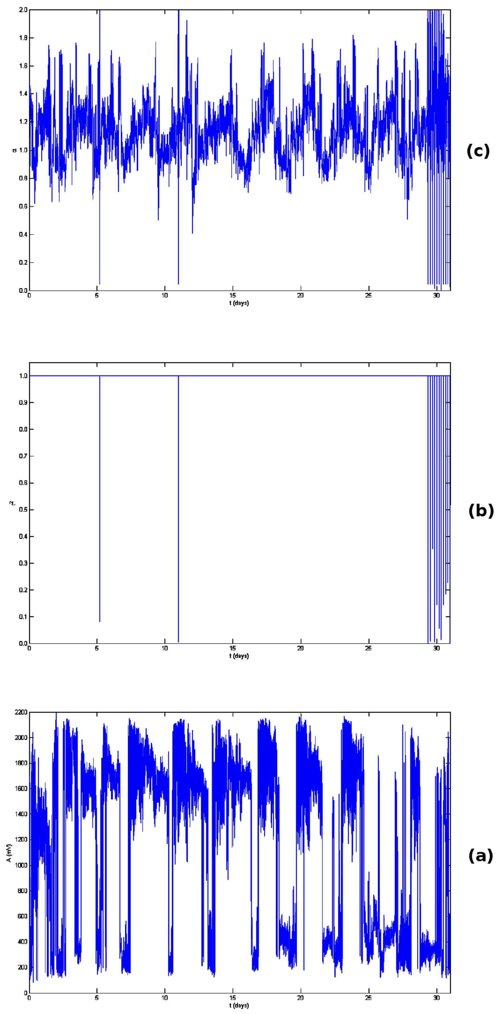
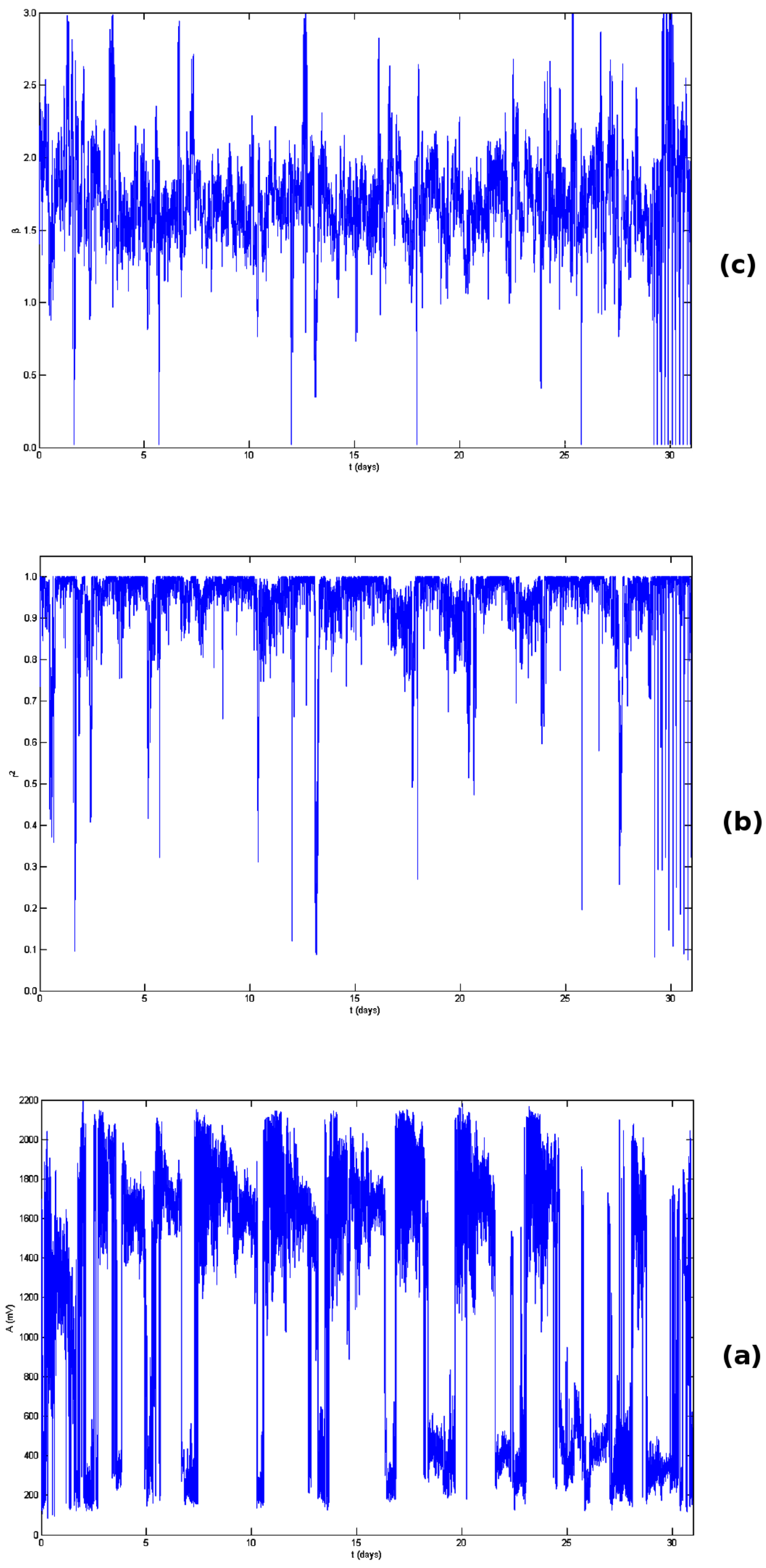
A total of 62,294 EM segments are recognized as of high predictability and of significant pre-earthquake fractal nature according to the findings of the fractal analysis technique. The fractal methods are very important in the study of pre-earthquake geosystems, because these exhibit intense fractal activity, both in space and time, according to extensive literature reports, e.g., [8,10,16].
From the argumentation given so far and the logic of Section 3.7 and Section 3.8, Figure 6 presents the stage 2 of the meta-analysis (subsection b of Section 3.8) in parallel to the earthquakes of Table 1 and Figure 2. As mentioned, Figure 6 presents all 13 possible combinations of fractal and long-memory methods (Section 3) per two, three, four and five techniques (stage 2 of meta-analysis) versus the 17 earthquakes of Table 1. Figure 6 is generated through GNU Octave® based on the stage 2 meta-analysis results of all methods. It should be emphasized that the meta-analysis (Section 3.8) is a fully computational method and thus, Figure 6 is a computer-generated plot in accordance to the results of the meta-analysis. It should be noted though that Figure 6 is an effort to visually present altogether a great amount of data that correspond to all combinations of the 13 different ASCII files of 1 s 1 rate each. As observed from Figure 6, earthquakes 1, 2 and 12 are concurrent with the black ‘+’ marks, which correspond to the combination of DFA versus all methods (combination of five methods). Earthquakes 7 and 13, 14 are almost concurrent with the black ‘+’ mark. A computational search within the corresponding meta-analysis ASCII files of DFA versus all methods, shows that all six earthquakes (earthquakes 1, 2, 7, 12, 13, 14) emit pre-seismic signs close in time, from some hours to less than an hour before their occurrence and close in space (all earthquakes have epicenters close to the EM station with the maximum distance 100.5 km for earthquake 1). Regarding the kHz radiation other investigators [8,10,11], have claimed that the kHz radiation is emitted from days up to some hours prior to earthquake occurrence and that when emitted, the material’s final catastrophe has started and the occurrence of the earthquake is inevitable. The findings of this paper for earthquakes 1, 2, 7, 12, 13 and 14 seem to support such an interpretation. In addition, earthquakes 3, 4, 5 and 6 are concurrent with the marks of all meta-analysis combinations except the black ‘+’ one, namely they are concurrent with all chaos analysis methods combinations per four, three and two. Via these combinations, earthquakes 3, 4, 5 and 6 emit signs of pre-seismicity just before their occurrence. The computational search within all combinations of meta-analysis ASCII files shows that earthquakes 3, 4, 5 and 6 emit pre-earthquake disturbances some hours prior to their occurrence. Also, earthquakes 8, 9, 10, 15, 16 and 17 are concurrent with the black ‘▽’ mark. This means that the combination of the methods of fractal analysis versus Higuchi’s and Sevcik’s (3 methods) support the view that earthquakes 8, 9, 10, 15, 16 and 17 emit pre-seismic signs shortly before their occurrence. According to the ASCII file of the stage 2 meta-analysis for the combination of the above methods, earthquakes 8, 9, 10, 15, 16 and 17 emit warnings some hours before their occurrence. Finally, earthquake 11 is concurrent with the magenta ‘⟐’ which corresponds to the combination of DFA versus Katz’s and Sevcik’s methods with similar interpretation.
The above findings provide noteworthy evidence that all earthquakes of Table 1 and Figure 2, emit pre-seismic warnings from some hours to several minutes before their occurrence time according to the recordings of the 3 kHz antennas. It is very important that the validity of the outcomes presented above, is supported by the meta-analysis of combination of at least three techniques. Significant is also that the methodological approach with the meta-analysis, provides much stronger arguments than the results of any of the methods separated. Several other papers have published results from separated methods (one or more), e.g., [8,10,11]. Advanced approaches based on methods comparison and significant theoretical background have been published as well, e.g., [22,23]. The approach of the present paper is, however, quite different and novel. This is because it is based on well-studied methods with extensive use in analysis of pre-seismic activity, importantly, in combination. As analyzed in several parts of this paper, by combining more than two chaos analysis and long-memory methods, the scientific evidence is much stronger when investigating the aspect that some kind of recorded pre-earthquake activity is possibly associated with earthquakes of the same time period and geographical area. Re-organizing the results under this view, very strong clues support the aspect that pre-seismic 3 kHz EM disturbances are emitted prior to earthquakes 1, 2, 7, 12, 13 and 14, since all combinations of methods are matched. The arguments for the 3 kHz EM activity prior to earthquakes 3, 4, 5 and 6, are quite strong since the combination of four, three and two methods support the pre-seismicity of these. Noteworthy evidence is given for earthquakes 8, 9, 10, 11, 15, 16 and 17 by three combinations of methods.
EM activity of the 3 kHz frequency emitted long before the occurrence of earthquakes (up to several days) has been reported also elsewhere [2,4,9,21]. Similar findings have been published for the MHz EM radiation [1,2,10,13,16,17,20,100] and for radon in soil variations [1,3,11,13,14,15,16,17,18]. After-effects have been reported by other investigators [please see reviews of [5,6,8,10,18]. Under this view, the meta-analysis results of Figure 6 that do not coincide with the earthquakes of Table 1 and Figure 2, might be probably pre-seismic effects emitted well before these earthquakes or can be post-seismic effects. As discussed in several papers [1,2,3,4,9,13,14,15,16,17,18,20,21,100], no one-to-one correspondence can be established between certain recorded activity and an ensuing earthquake. Moreover, as mentioned by [5], it is a serendipitous fact to record a very strong earthquake near a monitoring station and when found the evidence of an association are strong. Under these views, it is very hard to identify if the methods match in between the earthquakes of Table 1 and Figure 2, are post-seismic or pre-seismic. This is a limitation of the present methodology. On the other hand, the evidence for the precise or near matches are strong to noteworthy and this is a significant advantage of this methodology.
According to the argumentation given throughout the text, all earthquakes of this paper exhibited characteristic critical epochs of fractality and long-memory. As expressed in several publications [1,2,3,4,9,13,14,15,16,17,18,20,21], these epochs can be linked to the propagation of micro-cracks and cracks during the preparation phase of these earthquakes. At this phase, the micro-cracks are generated continuously and form larger cracks in a self-organizing and fractal manner. In this way, the small cracks constitute small scale fractal imitations of larger cracks and hence generate effective pathways that allow the propagation of pre-seismic EM anomalies [3,4,100]. During this process, critical Class-I fBm-profile EM disturbances are addressed. The results of Figure 3, Figure 4, Figure 5 and Figure 6, indicate this Class-I process since all critical segments exhibit persistent DFA exponents, fractal dimensions and power-law β -exponents. These are related to fBm modelling [3,4,16] which are produced by the 3 kHz EM generating geo-system of the Zakynthos area. During the preparation of the studied earthquakes, the focal area consists of a backbone of strong and large asperities that sustain the system and are modelled as fBm profiles. At a first stage, the fracture of the heterogeneous system in the focal area obstructs the backbone of asperities, but when the critical persistent meta-analysis matches of Figure 6 occur, the ‘siege’ of the asperities begin. Thereafter, the fracture starts and the unavoidable evolution of the process starts towards global failure. Finally, all critical warnings are of ensuing earthquakes and are revealed with the employed methods of this paper from the presented EM disturbances.

5. Conclusions

(1)
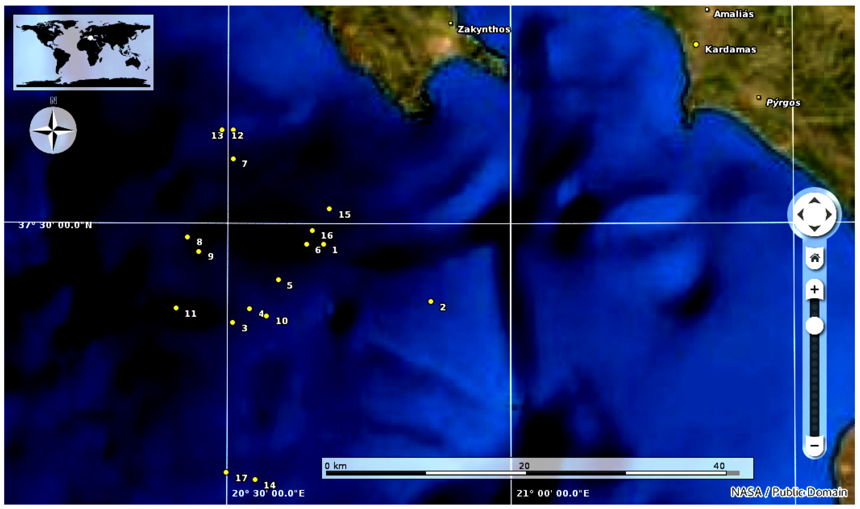
This paper focuses on the post-seismic activity of a strong M L = 6.6 earthquake occurred on 2018/10/25 in Zakynthos Island, Greece. The post-seismic period extends over one month and is based on 3 kHz EM disturbance measurements derived by a ground-station located at Kardamas, Ilia, Greece. Seventeen earthquakes are included in the study with magnitudes between M L = 4.5 and M L = 5.5 and depths between 3 km and 17 km with all epicenters near Zakynthos Island and Ilia.
(2)
Five different time-evolving chaos analysis methods are employed in the analysis. These methods are the detrended fluctuation analysis, the fractal dimension analysis with the methods of Higuchi, Katz and Sevcik and the power-law spectral fractal analysis. All these methods have been used with success in several pre-earthquake EM and radon signals in Greece.
(3)
A novel fully computational methodology (meta-analysis) is applied to the time-evolution ASCII outcomes of all five chaos analysis techniques. Via a two-stage process, all out-of-threshold ASCII data values are computationally searched and the common time instances of 13 possible combinations of five, four, three and two techniques are noted. Through this process combination results of significant value are produced.
(4)
Several persistent segments are found through DFA with exponents between 1.6 α 2.0 . Higuchi’s, Katz’s and Sevcik’s methods identify numerous segments with fractal dimensions 1.4 D 2.0 . Many segments with 2.2 β 3.0 are recognized by the fractal analysis method. All these thresholds refer to persistent fBm Class-I segments of high predictability and pre-seismic value.
(5)
Numerous combined meta-analysis segments are located with fractal behavior, dynamical complexity and long-memory. All these correspond to persistent fBm Class-I segments and are considered to be pre-earthquake footprints of high reliability.
(6)
Six of the 17 post-earthquakes are matched by all 13 selected combinations of five, four, three and two chaos analysis methods. Four earthquakes are matched by all combinations of four, three and two methods from the 13 combinations. The remaining seven earthquakes are matched by at least one combination of three methods. Activity within typical time windows among or after these earthquakes is reported as well.

Author Contributions

Conceptualization, D.N.; Data curation, E.P. and D.C.; Formal analysis, D.N., E.P. and D.C.; Investigation, D.N.; Methodology, D.N., I.V. and D.C.; Resources, G.P. and D.C.; Software, D.N. and D.C.; Supervision, D.N. and I.V.; Visualization, D.N.; Writing—original draft, D.N. and D.C.; Writing—review & editing, D.N., E.P., P.H.Y. and G.P. All authors have read and agreed to the published version of the manuscript.

Funding

This research received no external funding.

Conflicts of Interest

The authors declare no conflict of interest.

References

  1. Nikolopoulos, D.; Petraki, E.; Cantzos, D.; Yannakopoulos, P.H.; Panagiotaras, D.; Nomicos, C. Fractal Analysis of Pre-Seismic Electromagnetic and Radon Precursors: A Systematic Approach. J. Earth Sci. Clim. Chang. 2016, 7, 1–11. [Google Scholar]
  2. Nikolopoulos, D.; Cantzos, D.; Petraki, E.; Yannakopoulos, P.H.; Nomicos, C. Traces of long-memory in pre-seismic MHz electromagnetic time series-Part1: Investigation through the R/S analysis and time-evolving spectral fractals. J. Earth Sci. Clim. Chang. 2016, 7. [Google Scholar] [CrossRef] [Green Version]
  3. Nikolopoulos, D.; Matsoukas, C.; Yannakopoulos, P.H.; Petraki, E.; Cantzos, D.; Nomicos, C. Long-Memory and Fractal Trends in Variations of Environmental Radon in Soil: Results from Measurements in Lesvos Island in Greece. J. Earth Sci. Clim. Chang. 2018, 9, 1–11. [Google Scholar]
  4. Nikolopoulos, D.; Yannakopoulos, P.H.; Petraki, E.; Cantzos, D.; Nomicos, C. Long-Memory and Fractal Traces in kHz-MHz Electromagnetic Time Series Prior to the ML = 6.1, 12/6/2007 Lesvos, Greece Earthquake: Investigation through DFA and Time-Evolving Spectral Fractals. J. Earth Sci. Clim. Chang. 2018, 9, 1–15. [Google Scholar]
  5. Cicerone, R.; Ebel, J.; Britton, J. A systematic compilation of earthquake precursors. Tectonophysics 2009, 476, 371–396. [Google Scholar] [CrossRef]
  6. Ghosh, D.; Deb, A.; Sengupta, R. Anomalous radon emission as precursor of earthquake. J. Appl. Geophys. 2009, 187, 245–258. [Google Scholar] [CrossRef]
  7. Hayakawa, M.; Hobara, Y. Current status of seismo-electromagnetics for short-term earthquake prediction. Geomat. Nat. Hazards Risk 2010, 1, 115–155. [Google Scholar] [CrossRef]
  8. Uyeda, S.; Nagao, T.; Kamogawa, M. Short-term earthquake prediction: Current status of seismo-electromagnetics. Tectonophysics 2009, 470, 205–213. [Google Scholar] [CrossRef]
  9. Cantzos, D.; Nikolopoulos, D.; Petraki, E.; Yannakopoulos, P.H.; Nomicos, C. Earthquake precursory signatures in electromagnetic radiation measurements in terms of day-to-day fractal spectral exponent variation: Analysis of the eastern Aegean 13/04/2017–20/07/2017 seismic activity. J. Seismol. 2018, 22, 1499–1513. [Google Scholar] [CrossRef]
  10. Petraki, E.; Nikolopoulos, D.; Nomicos, C.; Stonham, J.; Cantzos, D.; Yannakopoulos, P.; Kottou, S. Electromagnetic Pre-earthquake Precursors: Mechanisms, Data and Models—A Review. J. Earth Sci. Clim. Chang. 2015, 6, 1–11. [Google Scholar]
  11. Petraki, E.; Nikolopoulos, D.; Panagiotaras, D.; Cantzos, D.; Yannakopoulos, P.; Nomicos, C.; Stonham, J. Radon-222: A Potential Short-Term Earthquake Precursor. J. Earth Sci. Clim. Chang. 2015, 6, 1–11. [Google Scholar]
  12. Khan, P.A.; Tripathi, S.C.; Mansoori, A.A.; Bhawre, P.; Purohit, P.K.; Gwal, A. Scientific efforts in the direction of successful Earthquake Prediction. Int. J. Geomat. Geosci. 2011, 1, 669–677. [Google Scholar]
  13. Nikolopoulos, D.; Petraki, E.; Marousaki, A.; Potirakis, S.; Koulouras, G.; Nomicos, C.; Panagiotaras, D.; Stonhamb, J.; Louizi, A. Environmental monitoring of radon in soil during a very seismically active period occurred in South West Greece. J. Environ. Monit. 2012, 14, 564–578. [Google Scholar] [CrossRef] [PubMed]
  14. Nikolopoulos, D.; Petraki, E.; Vogiannis, E.; Chaldeos, Y.; Giannakopoulos, P.; Kottou, S.; Nomicos, C.; Stonham, J. Traces of self-organisation and long-range memory in variations of environmental radon in soil: Comparative results from monitoring in Lesvos Island and Ileia (Greece). J. Radioanal. Nucl. Chem. 2014, 299, 203–219. [Google Scholar] [CrossRef]
  15. Nikolopoulos, D.; Petraki, E.; Nomicos, C.; Koulouras, G.; Kottou, S.; Yannakopoulos, P.H. Long-Memory Trends in Disturbances of Radon in Soil Prior ML = 5.1 Earthquakes of 17 November 2014 Greece. J. Earth Sci. Clim. Chang. 2015, 6, 1–11. [Google Scholar]
  16. Petraki, E. Electromagnetic Radiation and Radon-222 Gas Emissions as Precursors of Seismic Activity. Ph.D. Thesis, Department of Electronic and Computer Engineering, Brunel University, London, UK, 2016. [Google Scholar]
  17. Petraki, E.; Nikolopoulos, D.; Fotopoulos, A.; Panagiotaras, D.; Koulouras, G.; Zisos, A.; Nomicos, C.; Louizi, A.; Stonham, J. Self-organised critical features in soil radon and MHz electromagnetic disturbances: Results from environmental monitoring in Greece. Appl. Radiat. Isotop. 2013, 72, 39–53. [Google Scholar] [CrossRef]
  18. Petraki, E.; Nikolopoulos, D.; Fotopoulos, A.; Panagiotaras, D.; Nomicos, C.; Yannakopoulos, P.; Kottou, S.; Zisos, A.; Louizi, A.; Stonham, J. Long-range memory patterns in variations of environmental radon in soil. Anal. Methods 2013, 5, 4010–4020. [Google Scholar] [CrossRef]
  19. Balasis, G.; Daglis, I.; Papadimitriou, C.; Kalimeri, M.; Anastasiadis, A.; Eftaxias, K. Dynamical complexity in Dst time series using non-extensive Tsallis entropy. Geophys. Res. Lett. 2008, 35, 1–6. [Google Scholar] [CrossRef] [Green Version]
  20. Cantzos, D.; Nikolopoulos, D.; Petraki, E.; Nomicos, C.; Yannakopoulos, P.H.; Kottou, S. Identifying Long-Memory Trends in Pre-Seismic MHz Disturbances through Support Vector Machines. J. Earth. Sci. Clim. Chang. 2015, 6, 1–9. [Google Scholar]
  21. Cantzos, D.; Nikolopoulos, D.; Petraki, E.; Yannakopoulos, P.H.; Nomicos, C. Fractal Analysis, Information-Theoretic Similarities and SVM Classification for Multichannel, Multi-Frequency Pre-Seismic Electromagnetic Measurements. J. Earth. Sci. Clim. Chang. 2016, 7, 1–10. [Google Scholar] [CrossRef]
  22. Sarlis, N.; Skordas, E.; Varotsos, P.; Nagao, T.; Kamogawa, M.; Tanaka, H.; Uyeda, S. Minimum of the order parameter fluctuations of seismicity before major earthquakes in Japan. Proc. Natl. Acad. Sci. USA 2013, 110, 13734–13738. [Google Scholar] [CrossRef] [PubMed] [Green Version]
  23. Skordas, E.S. On the increase of the “non-uniform” scaling of the magnetic field variations before the M(w)9.0 earthquake in Japan in 2011. Chaos 2014, 24, 023131. [Google Scholar] [CrossRef] [PubMed]
  24. Smirnova, N.; Hayakawa, M. Fractal characteristics of the ground-observed ULF emissions in relation to geomagnetic and seismic activities. J. Atmos. Sol. Terr. Phys. 2007, 69, 1833–1841. [Google Scholar] [CrossRef]
  25. Smirnova, N.; Hayakawa, M.; Gotoh, K. Precursory behavior of fractal characteristics of the ULF electromagnetic fields in seismic active zones before strong earthquakes. Phys. Chem. Earth 2004, 29, 445–451. [Google Scholar] [CrossRef]
  26. Smirnova, N.A.; Kiyashchenko, D.A.T.; Troyan, V.N.; Hayakawa, M. Multifractal Approach to Study the Earthquake Precursory Signatures Using the Ground-Based Observations. Rev. Appl. Phys. 2013, 2, 3. [Google Scholar]
  27. Varotsos, P.; Sarlis, N.; Skordas, E. Scale-specific order parameter fluctuations of seismicity in natural time before mainshocks. Europhys. Lett. 2011, 96, 59002. [Google Scholar] [CrossRef] [Green Version]
  28. Varotsos, P.; Sarlis, N.; Skordas, E.S.; Christopoulos, G.; Lazaridou, M.S. Identifying the occurrence time of an impending mainshock: A very recent case. Earthq. Sci. 2015, 8, 215–222. [Google Scholar] [CrossRef] [Green Version]
  29. Varotsos, P.; Sarlis, N.; Skordas, E. Identifying the occurrence time of an impending major earthquake: A review. Earthq. Sci. 2017, 30, 209–218. [Google Scholar] [CrossRef]
  30. Parrot, M.; Tramutoli, V.; Liu, J.Y.; Pulinets, S.; Ouzounov, D.; Genzano, N.; Lisi, M.; Hattori, K.; Namgaladze, A. Atmospheric and ionospheric coupling phenomena related to large earthquakes. Nat. Hazards Earth Syst. Sci. Discuss 2016, 172, 1–30. [Google Scholar] [CrossRef] [Green Version]
  31. Ryu, K.; Parrot, M.; Kim, S.G.; Jeong, K.S.; Chae, J.S.; Pulinets, S.; Oyama, K.I. Suspected Seismo-Ionospheric Coupling Observed by Satellite Measurements and GPS TEC Related to the M7.9 Wenchuan Earthquake of 12 May 2008. J. Geophys. Res. Space Phys. 2014, 119, 1–19. [Google Scholar] [CrossRef] [Green Version]
  32. Kovachev, S.A. Results of seismological observations in the western Kaliningrad region and in the Baltik Sea water area, Izv. Phys. Solid Earth 2008, 44, 706–716. [Google Scholar] [CrossRef]
  33. Skarlatoudis, A.A.; Papazachos, C.B.; Margaris, B.N.; Theodulidis, N.; Papaioannou, C.; Kalogeras, I.; Scordilis, E.M.; Karakostas, V. Empirical peak ground-motion predictive relations for shallow earthquakes in Greece. Bull. Seismol. Soc. Am. 2003, 93, 2596–2603. [Google Scholar] [CrossRef]
  34. Hayakawa, M.; Kawate, R.; Molchanov, O.; Yumoto, K. Results of ultra-low-frequency magnetic field measurements during the Guam earthquake of 8 August 1993. Geophys. Res. Lett. 1996, 23, 241–244. [Google Scholar] [CrossRef]
  35. Hayakawa, M.; Itoh, T.; Hattori, K.; Yumoto, K. ULF electromagnetic precursors for an earthquake at Biak, Indonesia on February 17, 1996. Geophys. Res. Lett. 2000, 27, 1531–1534. [Google Scholar] [CrossRef]
  36. Hayakawa, M.; Ida, Y.; Gotoh, K. Multifractal analysis for the ULF geomagnetic data during the Guam earthquake. In Proceedings of the IEEE 6th International Symposium on Electromagnetic Compatibility and Electromagnetic Ecology, Saint Petersburg, Russia, 21–24 June 2005; pp. 239–243. [Google Scholar]
  37. Hayakawa, M.; Ida, Y.; Gotoh, K. Fractal (mono- and multi-) analysis for the ULF data during the 1993 Guam earthquake for the study of prefracture criticality. Curr. Dev. Theory Appl. Wavelets 2008, 2, 159–174. [Google Scholar]
  38. Varotsos, P.; Alexopoulos, K. Physical properties of the variations of the electric field of the earth preceding earthquakes, I. Tectonophysics 1984, 110, 73–98. [Google Scholar] [CrossRef]
  39. Varotsos, P.; Alexopoulos, K. Physical properties of the variations of the electric field of the earth preceding earthquakes, II. Tectonophysics 1984, 110, 99–125. [Google Scholar] [CrossRef]
  40. Varotsos, P.; Sarlis, N.; Lazaridou, M.B.N. Statistical evaluation of earthquake prediction results. Comments on the success rate and alarm rate. Acta Geophys. Pol. 1996, 44, 329–347. [Google Scholar]
  41. Varotsos, P.; Sarlis, N.; Eftaxias, K.; Lazaridou, M.B.N.; Makris, J.; Abdulla, A.; Kapiris, P. Prediction of the 6.6 Grevena-Kozani Earthquake of 13 May 1995. Phys. Chem. Earth 1999, 24, 115–121. [Google Scholar] [CrossRef]
  42. Varotsos, P.; Sarlis, N.; Skordas, E. Magnetic field variations associated with SES. The instrumentation used for investigating their detectability. Proc. Jpn. Acad. Ser. B 2001, 77, 87–92. [Google Scholar] [CrossRef] [Green Version]
  43. Varotsos, P.; Sarlis, N.; Skordas, E. Long-range correlations in the electric signals that precede rupture: Further investigations. Phys. Rev. E 2003, 67, 021109. [Google Scholar] [CrossRef] [PubMed] [Green Version]
  44. Varotsos, C.; Ondov, J.; Efstathiou, M. Scaling properties of air pollution in Athens, Greece and Baltimore. Md. Atmos. Environ. 2005, 39, 4041–4047. [Google Scholar] [CrossRef]
  45. Varotsos, C.A.; Ondov, J.M.; Cracknell, A.P.; Efstathiou, M.N.; Assimakopoulos, M.N. Long-range persistence in global aerosol index dynamics. Int. J. Remote Sens. 2006, 27, 3593–3603. [Google Scholar] [CrossRef]
  46. Varotsos, P.; Sarlis, N.; Skordas, E.; Lazaridou, M. Electric pulses some minutes before earthquake occurrences. Appl. Phys. Lett. 2007, 90, 1–3. [Google Scholar] [CrossRef] [Green Version]
  47. Varotsos, P.; Sarlis, N.; Skordas, E. Detrended Fluctuation Analysis of the magnetic and electric field variations that precede rupture. Chaos 2009, 19. [Google Scholar] [CrossRef] [Green Version]
  48. Yonaiguchi, N.; Ida, Y.; Hayakawa, M.; Masuda, S. Fractal analysis for VHF electromagnetic noises and the identification of preseismic signature of an earthquake. J. Atmos. Sol. Ter. Phy. 2007, 69, 1825–1832. [Google Scholar] [CrossRef]
  49. Nikolopoulos, D.; Moustris, K.; Petraki, E.; Koulougliotis, D.; Cantzos, D. Fractal and long-memory traces in PM10 time series in Athens, Greece. Environmnets 2019, 6, 29. [Google Scholar] [CrossRef] [Green Version]
  50. gredass. Available online: http://gredass.unife.it (accessed on 23 August 2019).
  51. INGV. 2007. Available online: http://diss.rm.ingv.it/diss/medtsunami/HTMLSourceZoneMaps/Hellenic_Arc.html (accessed on 23 August 2019).
  52. Lekas, A.; Fountoulis, I.; Papanikolaou, D. Intensity Distribution and Neotectonic Macrostructure Pyrgos Earthquake Data 26 March 1993, Greece. Nat. Hazards 2000, 21, 19–33. [Google Scholar] [CrossRef]
  53. NOA. Available online: http://www.gein.noa.gr/services/cat.html (accessed on 23 August 2019).
  54. USGS. Available online: http://earthquake.usgs.gov/earthquakes/map/ (accessed on 23 August 2019).
  55. Mandelbrot, B.B.; Ness, J.W.V. Fractional Brownian motions, fractional noises and applications. J. Soc. Ind. Appl. Math 1968, 10, 422–437. [Google Scholar] [CrossRef]
  56. Morales, I.O.; Landa, O.; Fossion, R.; Frank, A. Scale invariance, self-similarity and critical behaviour in classical and quantum system. J. Phys. Conf. Ser. 2012, 380. [Google Scholar] [CrossRef] [Green Version]
  57. Musa, M.; Ibrahim, K. Existence of long memory in ozone time series. Sains Malays. 2012, 41, 1367–1376. [Google Scholar]
  58. May, R.M. Simple mathematical models with very complicated dynamics. Nature 1976, 261, 459–467. [Google Scholar] [CrossRef] [PubMed]
  59. Sugihara, G.; May, R. Nonlinear forecasting as a way of distinguishing chaos from measurement error in time series. Nature 1990, 344, 734–741. [Google Scholar] [CrossRef] [PubMed]
  60. Hurst, H. Long term storage capacity of reservoirs. Trans. Am. Soc. Civ. Eng. 1951, 116, 770–808. [Google Scholar]
  61. Hurst, H.; Black, R.; Simaiki, Y. Long-term Storage: An Experimental Study; Constable: London, UK, 1965. [Google Scholar]
  62. Lopez, T.; Martınez-Gonzalez, C.; Manjarrez, J.; Plascencia, N.; Balankin, A. Fractal Analysis of EEG Signals in the Brain of Epileptic Rats, with and without Biocompatible Implanted Neuroreservoirs. AMM 2009, 15, 127–136. [Google Scholar] [CrossRef]
  63. Kilcik, A.; Anderson, C.; Rozelot, J.; Ye, H.; Sugihara, G.; Ozguc, A. Nonlinear Prediction of Solar Cycle 24. Astrophys. J. 2009, 693, 1173–1177. [Google Scholar] [CrossRef] [Green Version]
  64. Gilmore, M.; Yu, C.; Rhodes, T.; Peebles, W. Investigation of rescaled range analysis, the Hurst exponent, and long-time correlations in plasma turbulence. Phys. Plasmas 2002, 9, 1312–1317. [Google Scholar] [CrossRef] [Green Version]
  65. Granero, M.S.; Segovia, J.T.; Perez, J.G. Some comments on Hurst exponent and the long memory processes on capital Markets. Phys. A Stat. Mech. Appl. 2008, 387, 5543–5551. [Google Scholar] [CrossRef]
  66. Dattatreya, G. Hurst Parameter Estimation from Noisy Observations of Data Traffic Traces. In Proceedings of the 4th WSEAS International Conference on Electronics, Control and Signal Processing, Rio de Janeiro, Brazil, 25–27 April 2005; pp. 193–198. [Google Scholar]
  67. Fujinawa, Y.; Takahashi, K. Electromagnetic radiations associated with major earthquakes. Phys. Earth Planet. Inter. 1998, 105, 249–259. [Google Scholar] [CrossRef]
  68. Hayakawa, M. VLF/LF radio sounding of ionospheric perturbations associated with earthquakes. Sensors 2007, 7, 1141–1158. [Google Scholar] [CrossRef] [Green Version]
  69. Li, X.; Polygiannakis, J.; Kapiris, P.; Peratzakis, A.; Eftaxias, K.; Yao, X. Fractal spectral analysis of pre-epileptic seizures in terms of criticality. J. Neural Eng. 2005, 2, 11–16. [Google Scholar] [CrossRef] [PubMed] [Green Version]
  70. Rehman, S.; Siddiqi, A. Wavelet based Hurst exponent and fractal dimensional analysis of Saudi climatic dynamics. Chaos Solitons Fractals 2009, 39, 1081–1090. [Google Scholar] [CrossRef]
  71. Stanley, H.E. Powerlaws and universality. Nature 1995, 378, 597–600. [Google Scholar] [CrossRef]
  72. Stratonovich, R.L. Topics in the Theory of Random Noise; Gordon and Breach: New York, NY, USA, 1981. [Google Scholar]
  73. Chen, Z.; Ivanov, P.; Hu, K.; Stanley, H. Effect of nonstationarities on detrended fluctuation analysis. Phys. Rev. E 2002, 65, 1–15. [Google Scholar] [CrossRef] [PubMed] [Green Version]
  74. Hu, K.; Ivanov, P.C.; Chen, Z.; Hilton, M.F.; Stanley, H.E.; Shea, S. Non-random fluctuations and multi-scale dynamics regulation of human activity. Phys. A Stat. Mech. Appl. 2004, 337, 307–318. [Google Scholar] [CrossRef] [Green Version]
  75. Peng, C.; Mietus, J.; Havlin, S.; Stanley, H.; Goldberger, A. Long-range anti-correlations and non-Gaussian behavior of the heartbeat. Phys. Rev. Lett. 1993, 70, 1343–1346. [Google Scholar] [CrossRef]
  76. Peng, C.; Buldyrev, S.; Simons, M.; Havlin, S.; Stanley, H.; Goldberger, A. On the mosaic organization of DNA sequences. Phys. Rev. E 1994, 49, 1685–1689. [Google Scholar] [CrossRef] [Green Version]
  77. Peng, C.; Havlin, S.; Stanley, H.; Goldberger, A. Quantification of scaling exponents and crossover phenomena in nonstationary heartbeat time series. Chaos 1995, 5, 82–87. [Google Scholar] [CrossRef]
  78. Peng, C.; Hausdor, J.; Havlin, S.; Mietus, J.; Stanley, H.; Goldberger, A. Multiple-time scales analysis of physiological time series under neural control. Phys. A Stat. Mech. Appl. 1998, 249, 491–500. [Google Scholar] [CrossRef]
  79. Buldyrev, S.V.; Goldberger, A.L.; Havlin, S.; Mantegna, R.N.; Matsa, M.E.; Peng, C.K.; Simons, M.; Stanley, H.E. Long-range correlation properties of coding and noncoding DNA sequences: GenBank analysis. Phys. Rev. E Stat. Phys. 1995, 51, 5084–5091. [Google Scholar] [CrossRef]
  80. Ivanov, P.C.; Rosenblum, M.G.; Peng, C.K.; Mietus, J.E.; Havlin, S.; Stanley, H.E.; Goldberger, A.L. Multifractality in human heartbeat dynamics. Nature 1999, 399, 461–465. [Google Scholar] [CrossRef] [PubMed] [Green Version]
  81. Hu, K.; Ivanov, P.; Chen, Z.; Carpena, P.; Stanley, H. Effect of trends on Detrended Fluctuation Analysis. Phys. Rev. E 2001, 64, 1–19. [Google Scholar] [CrossRef] [PubMed] [Green Version]
  82. Ivanova, K.; Ausloos, M. Application of the detrended fluctuation analysis (DFA) method for describing cloud breaking. Phys. A Stat. Mech. Appl. 1999, 274, 349–354. [Google Scholar] [CrossRef]
  83. Koscielny-Bunde, E.; Bunde, A.; Havlin, S.; Roman, H.E.; Goldreich, Y.; Schellnhuberet, H. Indication of a Universal Persistence Law Governing Atmospheric Variability. Phys. Rev. Lett. 1998, 81, 729–732. [Google Scholar] [CrossRef]
  84. Vandewalle, N.; Ausloos, M. Coherent and random sequences in financial fluctuations. Phys. A Stat. Mech. Appl. 1997, 246, 454–459. [Google Scholar] [CrossRef]
  85. Varotsos, P.; Sarlis, N.; Skordas, E. Natural Time Analysis: The New View of Time. Precursory Seismic Electric Signals, Earthquakes and other Complex Time- Series; Springer: Berlin/Heidelberg, Germany, 2011. [Google Scholar]
  86. Varotsos, P.; Sarlis, N.; Skordas, E.; Lazaridou, M. Identifying sudden cardiac death risk and specifying its occurrence time by analyzing electrocardiograms in natural time. Appl. Phys. Lett. 2007, 91. [Google Scholar] [CrossRef]
  87. Nikolopoulos, D.; Valais, I.; Michail, C.; Bakas, A.; Fountzoula, C.; Cantzos, D.; Bhattacharyya, D.; Sianoudis, I.; Fountos, G.; Yannakopoulos, P.H.; et al. Radioluminescence properties of the CdSe/ZnS Quantum Dot nanocrystals with analysis of long-memory trends. Radiat. Meas. 2016, 92, 19–31. [Google Scholar] [CrossRef] [Green Version]
  88. Alam, A.; Wang, N.; Zhao, G.; Mehmood, T.; Nikolopoulos, D. Long-lasting patterns of radon in groundwater at Panzhihua, China: Results from DFA, fractal dimensions and residual radon concentration. Geochem. J. 2019, 53, 341–358. [Google Scholar] [CrossRef]
  89. Katz, M. Fractals and the analysis of waveforms. Comput. Biol. Med. 1988, 18, 145–156. [Google Scholar] [CrossRef]
  90. Raghavendra, B.; Dutt, D.N. Computing Fractal Dimension of Signals using Multiresolution Box-counting Method. Int. J. Electr. Comput. Energetic Electron. Commun. Eng. 2010, 4, 183–198. [Google Scholar]
  91. de la Torre, F.C.; Ramirez-Rojas, A.; Pavia-Miller, C.; Angulo-Brown, F.; Yepez, E.; Peralta, J. A comparison between spectral and fractal methods in electrotelluric time series. Rev. Mex. Fis. 1999, 45, 298–302. [Google Scholar]
  92. de la Torre, F.C.; Gonzaalez-Trejo, J.; Real-Ramírez, C.; Hoyos-Reyes, L. Fractal dimension algorithms and their application to time series associated with natural phenomena. J. Phys. Conf. Ser. 2013, 475, 1–10. [Google Scholar] [CrossRef]
  93. Higuchi, T. Approach to an irregular time series on basis of the fractal theory. Phys. D Nonlinear Phenom. 1988, 31, 277–283. [Google Scholar] [CrossRef]
  94. Sevcik, C. On fractal dimension of waveforms. Chaos Solit. Fract. 2006, 27, 579–580. [Google Scholar] [CrossRef]
  95. Gotoh, K.; Hayakawa, M.; Smirnova, N. Fractal analysis of the ULF geomagnetic data obtained at Izu Peninsula, Japan in relation to the nearby earthquake swarm of June-August 2000. Nat. Haz. Earth Sys. 2003, 3, 229–234. [Google Scholar] [CrossRef]
  96. Gotoh, K.; Hayakawa, M.; Smirnova, N.; Hattori, K. Fractal analysis of seismogenic ULF emissions. Phys. Chem. Earth 2004, 29, 419–424. [Google Scholar] [CrossRef]
  97. Ida, Y.; Hayakawa, M. Fractal analysis for the ULF data during the 1993 Guam earthquake to study prefracture criticality. Nonlinear Process. Geophys. 2006, 13, 409–412. [Google Scholar] [CrossRef] [Green Version]
  98. Telesca, L.; Lasaponara, R. Vegetational patterns in burned and unburned areas investigated by using the detrended fluctuation analysis. Phys. A Stat. Mech. Appl. 2006, 368, 531–535. [Google Scholar] [CrossRef]
  99. Telesca, L.; Lapenna, V.; Vallianatos, F. Monofractal and multifractal approaches in investigating scaling properties in temporal patterns of the 1983–2000 seismicity in the Western Corinth Graben, Greece. Phys. Earth Planet. Int. 2002, 131, 63–79. [Google Scholar] [CrossRef]
  100. Petraki, E.; Nikolopoulos, D.; Chaldeos, Y.; Koulouras, G.; Nomicos, C.; Yannakopoulos, P.H.; Kottou, S.; Stonham, J. Fractal evolution of MHz electromagnetic signals prior to earthquakes: Results collected in Greece during 2009. Geomat. Nat. Hazards Risk 2016, 7, 550–564. [Google Scholar] [CrossRef] [Green Version]
Figure 1. Geological background of Greece. The figure shows the seismic plates that surround Greece and the Trenches in yellow and orange.
Geosciences 10 00235 g001
Figure 2. The epicenters of the earthquakes of Table 1 occurred between 2018/10/26–2018/11/26 within circle of 101 km radius centered at the Kardamas station (21.34° E, 37.76° N). The identifiers are according to Table 1.
Geosciences 10 00235 g002
Figure 3. Results of DFA. From bottom to top: (a) The EM time series; (b) The Spearman’s correlation coefficient of the goodness of the linear fit of F ( n ) versus n in every 1024-sample window; (c) The scaling exponent α (DFA slope). Horizontal axis is in days from the beginning of measurements (2018/10/26). The measurement sampling rate is 1 s 1 .
Geosciences 10 00235 g003
Figure 4. Results from fractal dimension analysis. From bottom to top: (a) The EM time series and the fractal dimensions according to the algorithms of (b) Katz (KFD); (c) Higuchi (HFD) and (d) Sevcik (SFD). Horizontal axis is in days from the beginning of measurements (2018/10/26). The measurement sampling rate is 1 s 1 .
Geosciences 10 00235 g004
Figure 5. Results from fractal analysis: From bottom to top: (a) The EM time series; (b) The Spearman’s correlation coefficient of the goodness of the linear fit of Equation (18) in every 1024-sample window; (c) The time evolution of power-law β exponent. Horizontal axis is in days from the beginning of measurements (2018/10/26). The measurement sampling rate is 1 s 1 .
Geosciences 10 00235 g005
Figure 6. Overview of the full computational meta-analysis results by all 13 selected combinations of chaos analysis methods per five, four, three and two methods. From top to bottom: ‘+’ (black): DFA versus all methods (5 techniques); ‘⊙’ (red): DFA versus all fractal dimension techniques (4 techniques); ‘*’ (green): Fractal analysis versus all fractal dimension techniques (4 techniques); ‘.’ (blue): DFA versus Higuchi’s and Katz’s methods (3 techniques); ‘⊡’ (yellow): DFA versus Higuchi’s and Sevcik’s methods (3 techniques); ‘⟐’ (magenta): DFA versus Katz’s and Sevcik’s methods (3 techniques); ‘▽’ (cyan): Fractal analysis versus Higuchi’s and Katz’s methods (3 techniques); ‘▽’ (black): Fractal analysis versus Higuchi’s and Sevcik’s methods (3 techniques); ‘▷’ (red): Fractal analysis versus Katz’s and Sevcik’s methods (3 techniques); ‘◁’ (green): Higuchi’s versus Katz’s and Sevcik’s methods (3 techniques); ‘⬠’ (blue): Sevcik’s versus Katz’s and Higuchi’s methods (3 techniques); ‘*’ (yellow): Katz’s versus Higuchi’s and Sevcik’s methods (3 techniques); ‘+’ (magenta): DFA versus fractal analysis (2 techniques). Horizontal axis is in actual dates. The vertical axis expresses the M L magnitude of the earthquakes of Table 1 and Figure 2. The stem lines (black with green circle and red outline) correspond to the numbering of the earthquakes of Table 1 (1–17).
Geosciences 10 00235 g006
Table 1. Earthquakes included in the present study in chronological sequence. Actual dates and corresponding Julian Days (JD) of 2009 are also given. Abbreviations: M L : Local Magnitude, Lt: Latitude, Lg: Longitude, Depth: Epicentral depth, Dist: Distance of the earthquake epicenter from the Kardamas station. All data, except symbol and JD, are retrieved by [53].
iSymbolDateGMTJD M L Lt (°N)Lg (°E)Depth (km)Dist (km)
1.EQ12018/10/2600:13:392994.537.4720.670667.2
2EQ22018/10/2601:06:032994.537.3920.860659.0
3.EQ32018/10/2605:48:362994.837.3620.510885.6
4.EQ42018/10/2612:41:132994.637.3820.540582.2
5.EQ52018/10/2616:07:092994.537.4220.590776.1
6.EQ62018/10/2705:28:463004.637.4720.640569.6
7EQ72018/10/3002:59:593035.437.5920.510775.5
8.EQ82018/10/3008:32:263034.837.4820.431186.0
9.EQ92018/10/3015:12:023035.537.4620.450685.2
10.EQ102018/11/0102:44:483054.637.3720.571180.5
11.EQ112018/11/0403:12:443084.937.3820.410592.2
12.EQ122018/11/0506:46:123094.537.6320.490876.2
13.EQ132018/11/1123:38:353154.837.6320.510774.4
14.EQ142018/11/1206:50:273164.737.1420.551098.1
15.EQ152018/11/1509:02:053194.937.5220.681763.9
16.EQ162018/11/1509:09:263194.537.4920.650767.8
17.EQ172018/11/1913:05:543235.137.1520.5010100.5

