Down-Sampling of Large LiDAR Dataset in the Context of Off-Road Objects Extraction

Abstract

Nowadays, LiDAR (Light Detection and Ranging) is used in many fields, such as transportation. Thanks to the recent technological improvements, the current generation of LiDAR mapping instruments available on the market allows to acquire up to millions of three-dimensional (3D) points per second. On the one hand, such improvements allowed the development of LiDAR-based systems with increased productivity, enabling the quick acquisition of detailed 3D descriptions of the objects of interest. However, on the other hand, the extraction of the information of interest from such huge amount of acquired data can be quite challenging and time demanding. Motivated by such observation, this paper proposes the use of the Optimum Dataset method in order to ease and speed up the information extraction phase by significantly reducing the size of the acquired dataset while preserving (retain) the information of interest. This paper focuses on the data reduction of LiDAR datasets acquired on roads, with the goal of extraction the off-road objects. Mostly motivated by the need of mapping roads and quickly determining car position along a road, the development of efficient methods for the extraction of such kind of information is becoming a hot topic in the research community.

1. Introduction

Thanks to the high accuracy and reliability of Light Detection and Ranging (LiDAR) scanners, the use of such instruments has become the state-of-the-art of static and mobile mapping systems during the past decade. Given the possibility of using LiDAR sensors in both terrestrial and aerial surveys (Terrestrial Laser Scanning (TLS), Mobile Laser Scanning (MLS), Airborne Laser Scanning (ALS)), the number of applications exploiting such kind of technology is continuously increasing, including nowadays several fields such as civil and structural engineering [1], forestry and environmental protection [2], road engineering [3], and assisted/autonomous driving. Many possible applications include, for instance, infrastructure documentation, construction of roads and highways [4], production of digital terrain models [5], inventory mapping [6], design of streetscape [7], extraction of traffic signs and buildings [8], safety improvements [9], and more recently, even the creation of three-dimensional (3D) models to support visual effects in the film industry [10].

The quest for fast and detailed 3D spatial data acquisitions led to the development of LiDAR systems gathering information at a high data rate, up to millions of points per second in the current generation of LiDAR scanners. Furthermore, since due to occlusions some objects are not properly mapped by a single LiDAR mobile scanner, nowadays MLS systems are often provided with several LiDAR instruments acquiring data simultaneously but along different directions. On the one hand, the use of such multiple LiDAR systems ensures the collection of a spatially more complete dataset, on the other hand, the size of the collected point cloud quickly becomes huge.

In fact, there are several projects that use LiDAR systems for infrastructure documentation at large scales, such as transportation/power lines mapping and monitoring and inspection on large areas, possibly up to national scale. Moreover, some recent applications, such as autonomous/assisted driving, require the real time analysis of the acquired data in order to extract the information of interest. Such kind of requirement, in addition to the already mentioned need of properly dealing with huge amount of data, motivate the development of computationally efficient ways for effectively and timely processing the collected data.

In accordance with the above observations, this work proposes the use of Optimum Dataset (OptD) method in order to ease and speed up the process of off-road object (such as traffic signs, power lines, light poles, roadside trees) extraction from LiDAR data collected by MLS/ALS.

Fast and automatic detection of on-road and off-road objects from LIDAR datasets is very important for intelligent transportation infrastructure management as well as for driver assistance and for safety warning systems [11,12]. Several approaches have been recently proposed for the automatic detection of such objects. As LiDAR provides both geometric and radiometric information about the measured points (the so-called intensity depends on the physicochemical properties of the scanned surface, such as the roughness, color, and humidity [13]); hence, both of them can be employed in the object detection process [14]. A method combining unsupervised k-means, geometric and reflectivity characteristics to identify road points, traffic signs, and light poles has been developed in [14]. Machine learning methods have been employed in [8] to recognize on/off-road objects in urban environments. Laplacian smoothing, k-nearest neighbors graph, and Principal Component Analysis (PCA) have also been used to detect off-road objects [15,16].

All the methods mentioned above were applied to the complete collected LiDAR dataset; however, since the computational burden of the object detection algorithm is largely dependent on the dataset size, the use of such methods on the entire LiDAR point cloud can be computationally quite inefficient, in particular when dealing with huge datasets and quite stringent processing time requirements. In such cases, an automatic data optimization step can be conveniently applied in order to reduce the dataset size before applying the object detection algorithm. Such optimization phase shall clearly be a smart data reduction step: the rationale is that of retaining most of the points related to the objects of interest (e.g., traffic signs, light poles) while discarding most of the others (points in areas of low interest, such as on roads and pavements). In this way, the successive off-road object detection phase can be speeded up thanks to the dramatic data reduction, whereas the off-road object detection performance is almost invariant.

Several methods have already been proposed in the literature in order to reduce large LIDAR datasets, such as generation [17,18] algorithms based on the estimation of surface curvature radius [19,20], and octree-balanced density down-sampling [21]. It is worth to notice that some of these data reduction methods are implemented in laser scanning processing software, e.g., Leica Cyclone, CloudCompare.

The goal of this work is to investigate the effectiveness of the OptD method, applied with a properly defined optimization criterion, in order to achieve a suitable data reduction. The obtained results are compared with those of the random down-sampling implemented in the CloudCompare software.

2. Methods

2.1. Review on Road Object Detection

The object detection problem refers to the computer capability of identifying and locating objects in a scene. Traditionally, most of the object detection methods were based on the use of machine learning methods, applied on pre-determined features, which were supposed to properly characterize the objects of interest. Nowadays, deep learning approaches have been shown to be more effective in a number of cases (e.g., Regional Convolutional Neural Network (RCNN)), Fast-RCNN, Faster-RCNN, “You Only Look Once” (YOLO). Differently from classical machine learning techniques, deep learning approaches aim at automatically determining the most suitable (typically high-level) features, which are usually learned along with the desired classifier. A more detailed review on the object detection history and recent developments is presented in [22].

Despite that object detection methods were originally deployed as image analysis algorithms (e.g., they aimed to detect objects based to the visual information provided by cameras), the recent spread of 3D acquisition and visualization technologies encourages the development of object detection methods based on 3D information, e.g., on 3D point clouds. In particular, as long as road object detection is concerned, the role of 3D data processing and object detection is one of fundamental importance: indeed, several applications in this context (e.g., infrastructure mapping and documentation, autonomous/assisted driving) are based on the use of MLS [23,24].

On-road and off-road objects are usually divided in several sub-categories, as described in the following. On-road objects are typically classified into five categories: road surfaces, road markings, driving lines, road cracks, and road manholes. Differently, off-road objects, which are those of interest in this study, are usually classified into four categories [23]:

• Traffic Sign (TS)
• Light Pole (LP)
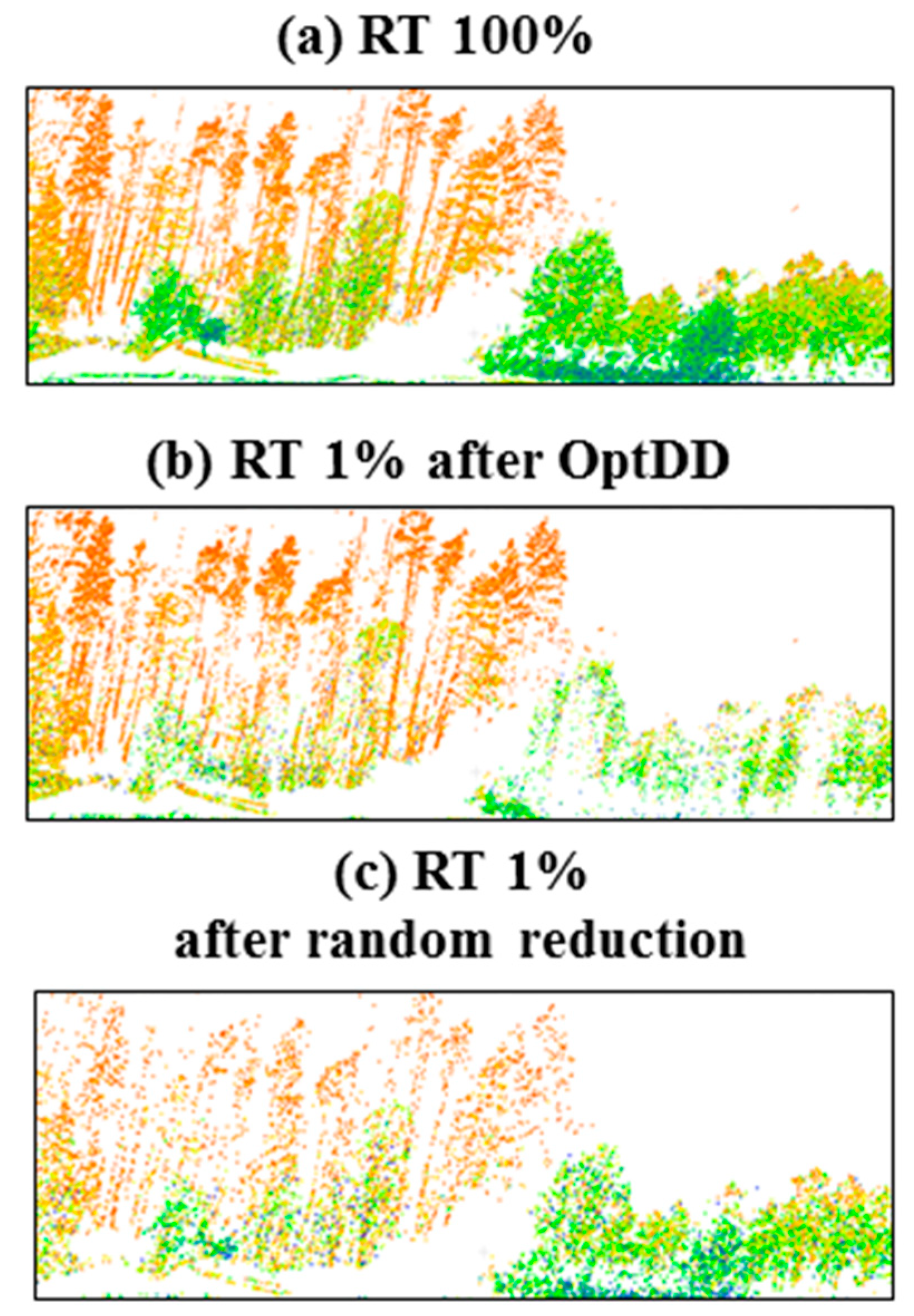
• Roadside Trees (RT)
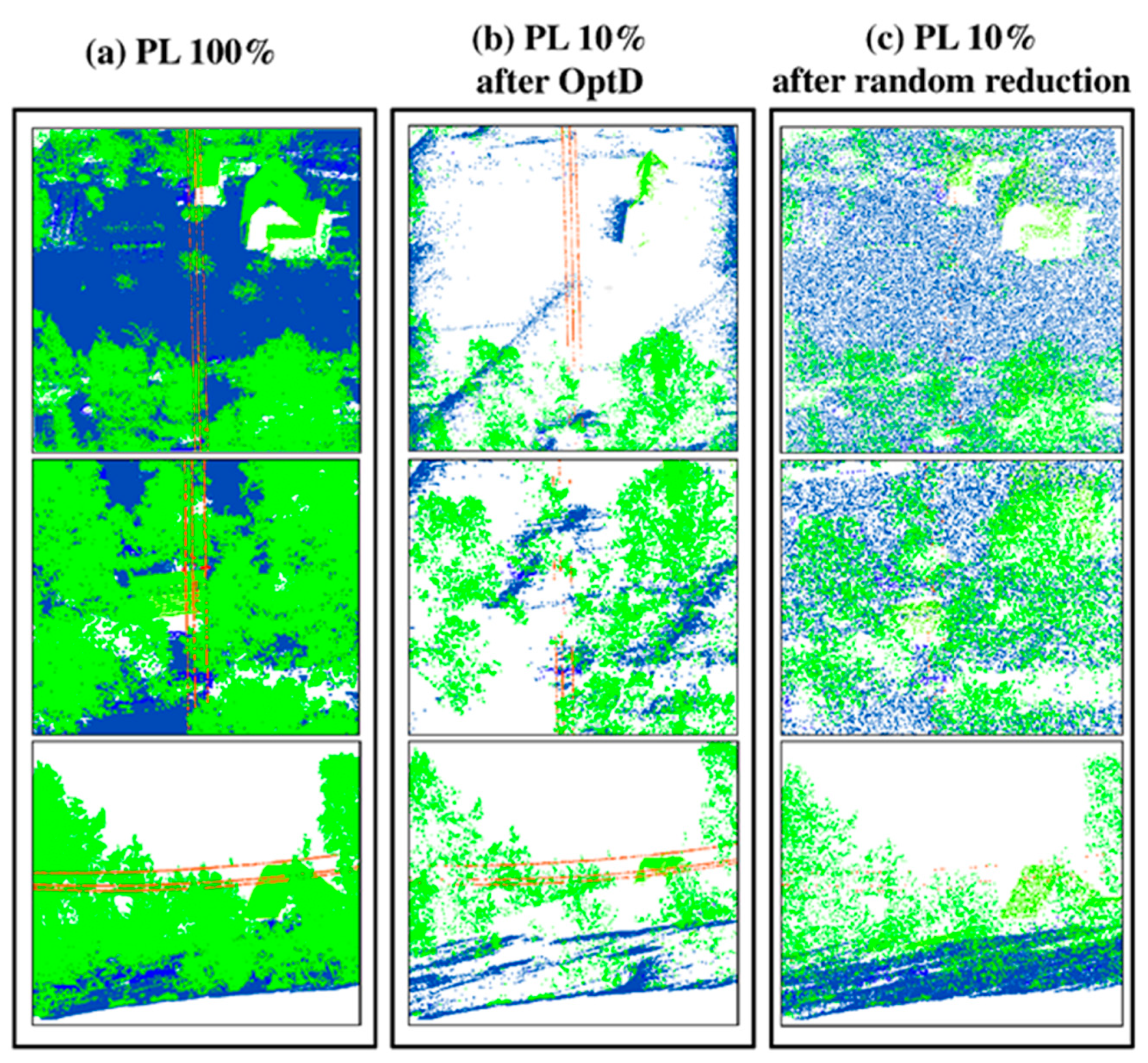
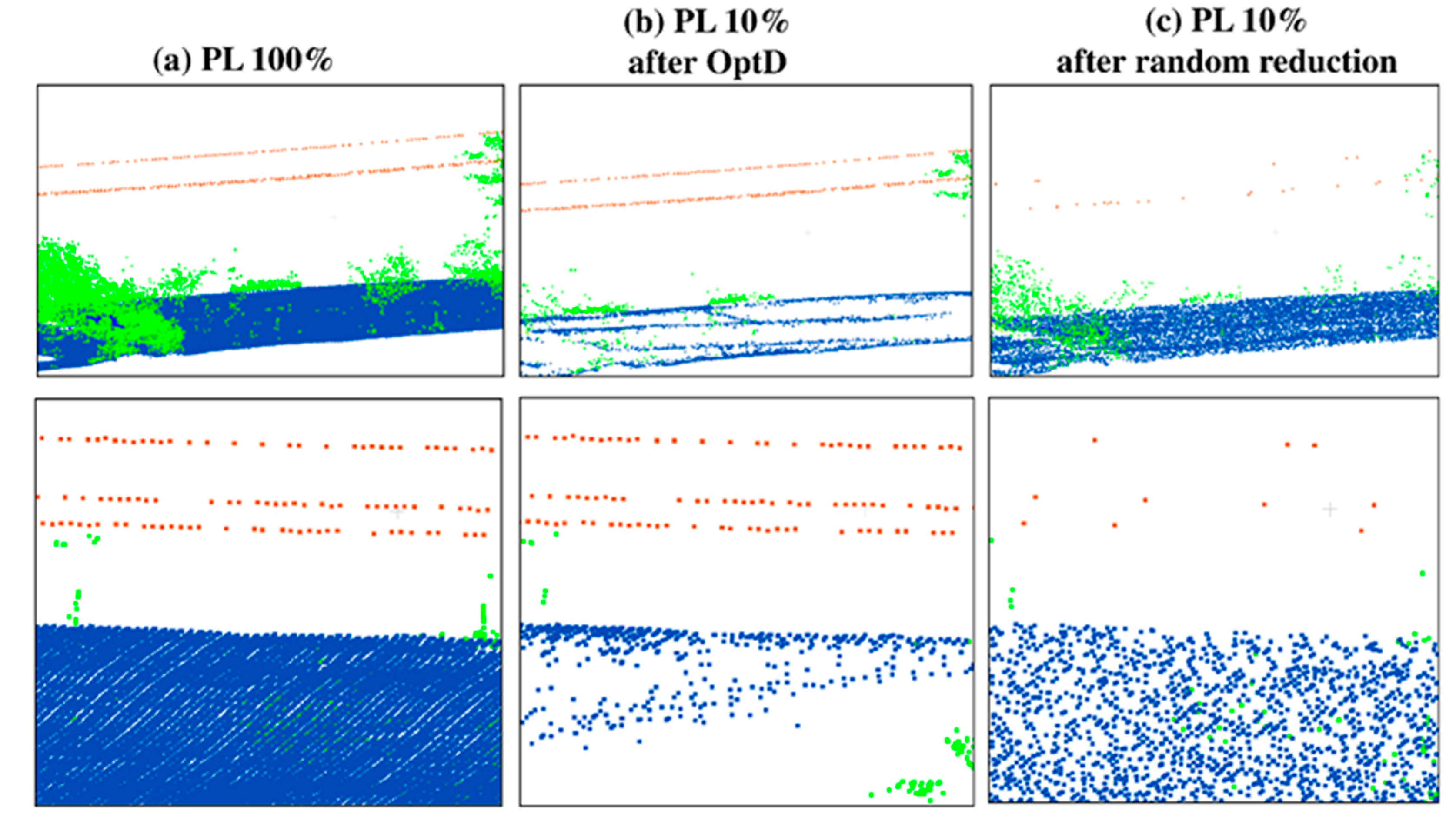
• Power Lines (PL)

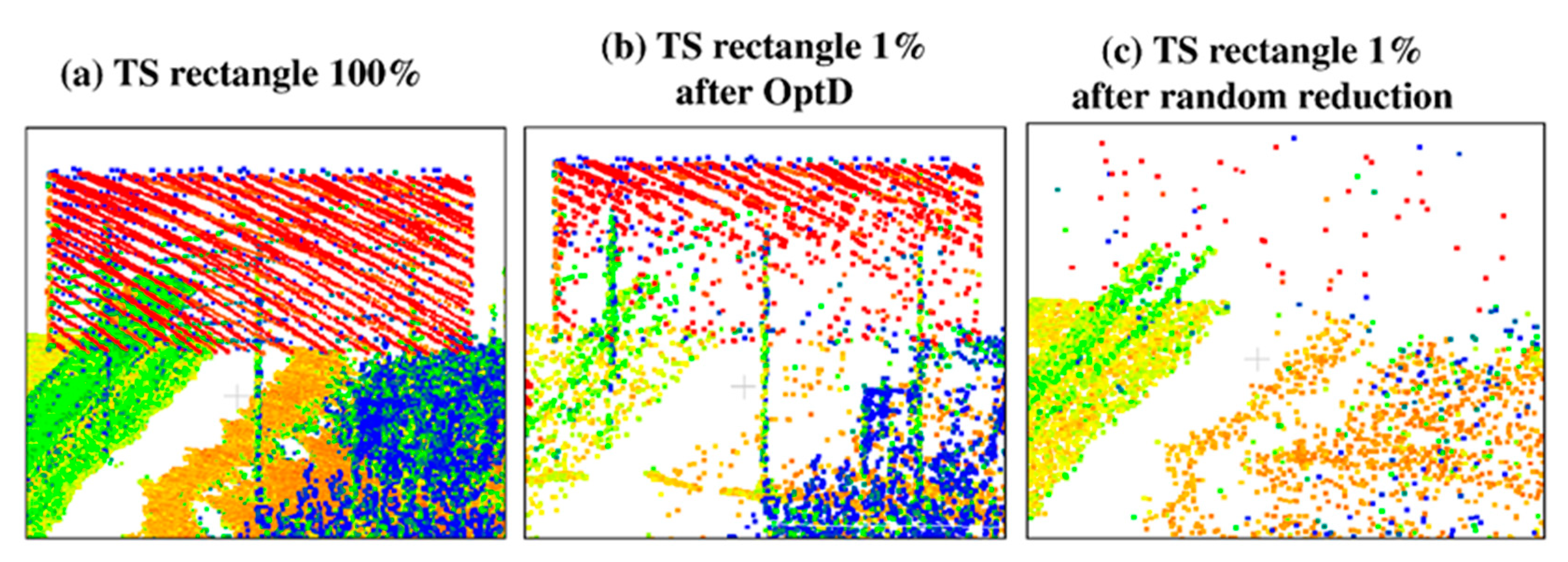
TS detection and recognition methods typically exploit both the geometric and radiometric characteristics of each traffic sign. The geometric shape of a traffic sign is usually highly regular (triangle, rectangle, or circle) and its position with respect to the road is quite standard: it is usually installed on the side of a road, at a specific height, approximately perpendicular to the ground, and parallel to other pole-like objects. Furthermore, its surface is planar, it is made with a metallic highly reflective material and covered with reflective paint. Since an imagery acquisition system is typically used in combination with the laser scanner, TS recognition is usually based on a three-step procedure: (1) traffic sign detection on the 3D dataset, (2) identification of the two-dimensional (2D) area in the camera imagery corresponding to the detected traffic sign, (3) use of image-based recognition methods on the determined 2D area [25]. Such recognition methods are typically based on either machine learning or deep learning approaches, where the latter have recently shown a superior performance in many applications. Clearly, the performance of the TS recognition phase is strictly related to the accuracy of the previous detection phase [23].

Two categories of light pole detection algorithms can be distinguished: knowledge-driven and data-driven methods. First, knowledge-driven methods can be classified in two sub-categories: matching-based and rule-based extraction. Matching-based extraction is based on the use of a pre-selected pole model that is matched with the extracted object. Since it is quite time consuming, it cannot be considered to be a viable method when dealing with large-volume data processing [26]. Differently, rule-based extraction applies several rules, typically based on the geometric and spatial characteristics of light poles (e.g., location, radius, height), in order to remove any object different from a light-pole. Clearly, the number of rules to be applied, as well as the spatial data distribution, exert a significant impact on the efficiency of this kind of object extraction. In data-driven methods, a set of features is typically extracted from the dataset and used to characterize the objects of interest: as often done in machine learning, a massive and properly labelled training dataset is used to train a suitable light pole extractor [24,27].

Roadside tree detection from MLS point clouds is typically done by means of either rule-based [28] or deep learning methods [29,30].

2.2. Optimum Dataset Method

This subsection shortly summarizes the main characteristics of the OptD method, mostly to properly highlight the changes applied here to the implementation previously used in other works. We refer the reader to [31,32,33,34] for a more detailed algorithmic description of the method.

The goal of the OptD method is to reduce the size of a point cloud while preserving as much as possible the information that is necessary for the correct implementation of the task of interest (e.g., the computation of a digital terrain model, a digital surface model, an inventory, or a thematic map). To achieve this aim, the selection of a proper optimization criterion is fundamental in order to guarantee the desired data reduction while retaining the information of interest.

The first stage of the OptD method begins with the question to the user to set a proper optimization criterion (f). Different optimization criteria can be used for reduction, for example, the average error of the dataset after the reduction exactly indicated number of points or percent of points after reduction. In this paper, the optimization criterion in the form of a percentage of points was used. Then the OptD method starts determining the area of interest, i.e., the minimum and maximum horizontal coordinates. Then, the determined rectangular area is partitioned into strips. The width of the strips L is automatically optimized in subsequent iterations of the OptD algorithm. The analysis of the points belonging to each of the strips includes the application of the selected cartographic generalization method [35,36], which has to be pre-selected by the user. The result of the generalization depends on the value of the tolerance range t, which is automatically updated in subsequent iterations of the algorithm until the condition expressed by the desired optimization criterion is met.

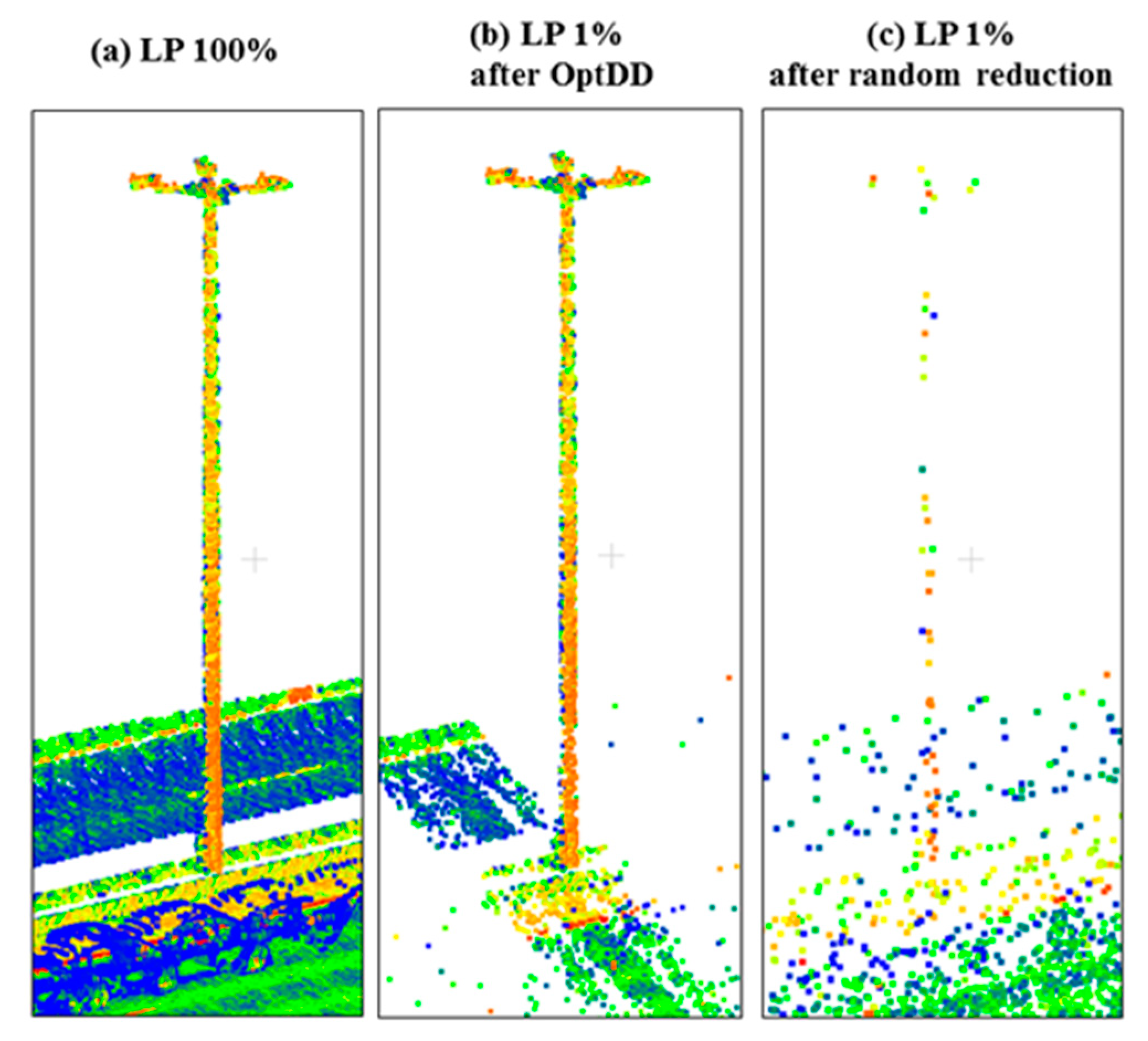
A change with respect to the OptD method used in previous works is applied here in the application of the generalization method. More specifically, given the importance in this work of high and relatively thin elements such as LPs, the generalization method is changed in order to retain a higher number of points in correspondence of high objects.

In practice, when several points are found with different vertical coordinates, but quite similar horizontal coordinates and intensity value, then the data reduction rate is reduced in such area by lowering the value of the tolerance range. Moreover, the hitherto operation is modified in order to avoid any change due to the OptD method to the nature of vertical objects (e.g., LP, the tube on which the TS is mounted). This preserve the possibility of correctly identifying the object even after applying the data reduction.

It is worth to notice that the only user-dependent actions in the application of the OptD method are entering the optimization criterion and the selection of the generalization method, whereas all the rest of the procedure is completely automatic (e.g., determining the strip width and the tolerance range).

Summarizing above, the OptD method for off-road objects extraction is carried out in the following stages:

• Reading the LiDAR dataset.
• Setting the optimization criterion (f%).
• Determination of the processing area. In this way, a rectangular processing area is created, which is divided during the processing with OptD into strips (L).
• Each strip is analyzed separately. In each strip there are measuring points that form a curve. The curve is generalized with the use of generalization methods, here: Douglas-Peucker method [35]. The generation of lines created by points in the strips is always performed in the OXZ or OYZ plane. Thus, the changes are detected by analyzing the geometry. In this stage, the tolerance range value (t) is determined.
• The end of OptD processing occurs when the generalization method is applied in all strips. The saved dataset meets the optimization criterion set in stage 2. The values L and t are changed during the iteration until the output dataset meets the optimization criterion.
• The optimum LiDAR point cloud is saved. Then, the user can use the reduced and classified dataset for visualization.

2.3. Workflow

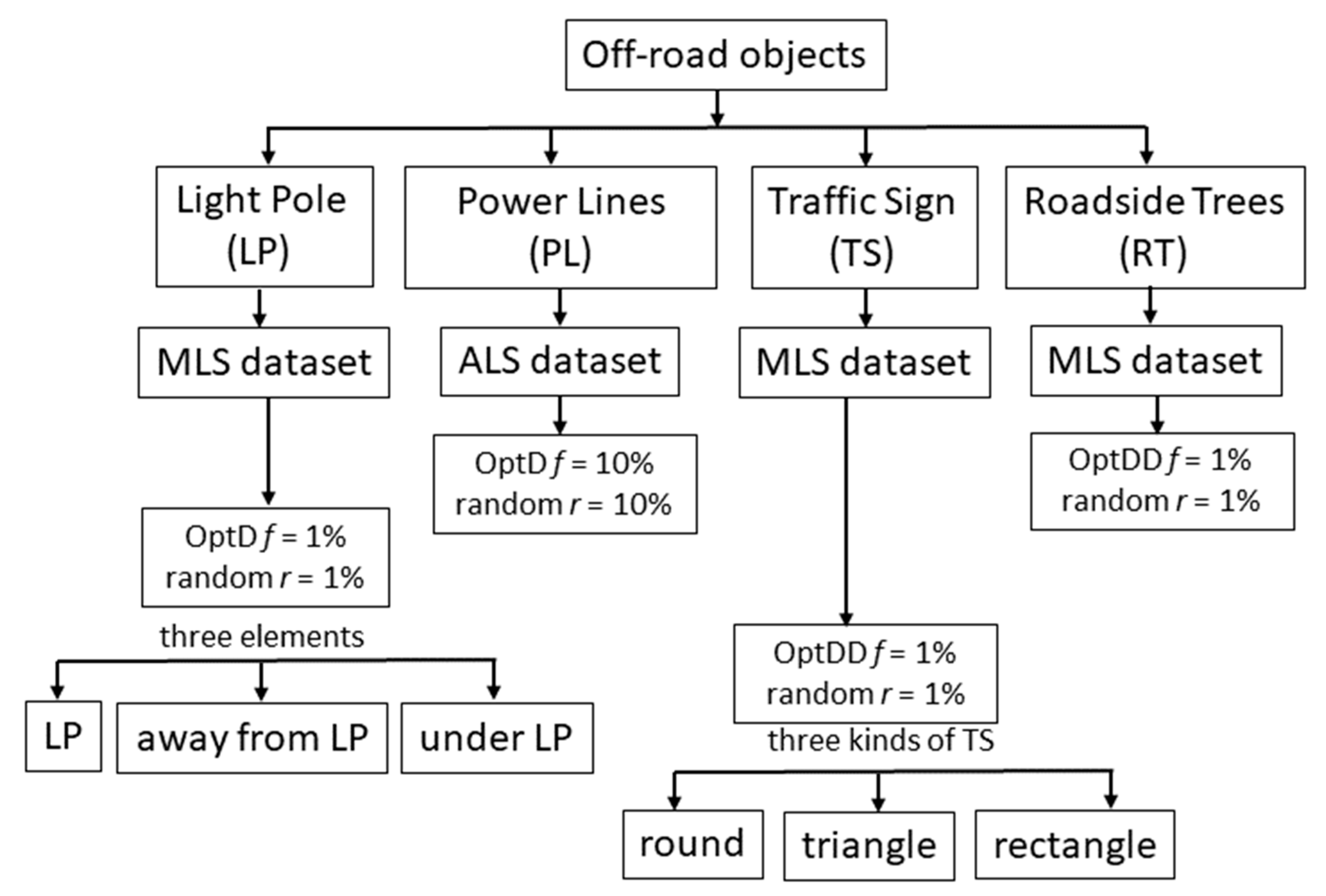
In this work the OptD method is used for the data reduction of datasets including off-road objects. In particular, the behavior of OptD is checked in four cases corresponding to the previously mentioned four categories of off-road objects. In all considered cases MLS datasets have been used in the tests done in this paper. It is worth to notice that, in the PL case, power lines were hardly noticeable in the MLS dataset. Therefore, ALS dataset has been considered in the results shown in this work.

In all the cases, the dataset has been processed with OptD and, for comparison, with the built-in data reduction function in CloudCompare (random cloud sub-sampling), by using the workflows summarized in the following.

Workflow with OptD:

• Import dataset (—input *.txt).
• Data reduction (—OptD.bat, —data reduction according to the selected optimization criterion f%).
• Export dataset after reduction (—output *.txt).

Workflow with CloudCompare:

• Import dataset (open ASCII file *.txt).
• Data reduction (cloud sub-sampling, random method with criterion r%).
• Export dataset after reduction (save as ASCII cloud *.txt).

The scheme in Figure 1 shows the different case studies of off-road objects considered in this work.

Given the different scanning resolution of the MLS and ALS datasets, and given the quite small number of PL points in any of the considered datasets (both MLS and ALS), a different reduction rate has been applied: MLS datasets, used in the LP and TS tests, have been reduced at 1% of the original size, whereas 10% of reduction rate (defined as the ratio between the reduced and the original size) has been used in the case of ALS.

The comparison with the CloudCompare results has been done by considering the same reduction rates used for the OptD method.

2.4. LiDAR Datasets

2.4.1. MLS Dataset

The MLS data acquisition was carried out by GEOPARTNER (www.geopartner.gda.pl) in 2017, which used the Topcon IP-S3 mobile mapping system. Despite being quite small, light, and easy to handle, Topcon IP-S3 provides high density and precision point clouds combined with high resolution panoramas. Precise positioning and attitude in a dynamic environment are done thanks to the combination of information from IMU (Inertial Measurement Unit), GNSS (Global Navigation Satellite System) receiver (GPS and GLObal NAvigation Satellite System (GLONASS)), and a vehicle odometer. Furthermore, it has a six-lens digital camera system that provides 360-degree high resolution spherical images. Concerning the laser scanner unit, the scanning rate is 700,000 pulses per second. There are 32 internal lasers covering the full 360 degrees around the system, each from a slightly different viewing angle, which minimizes gaps in the point cloud. All post processing trajectories and georeferencing scans and images are performed in Mobile Master Office software.

The MLS dataset considered in this paper is shown in Figure 2. The presented point cloud is not classified, and the colors of the points result from the intensity.

The MLS dataset has been processed by means of OptD and random reduction in CloudCompare (CC), leading to the results shown in

Table 1. Characteristics of the MLS dataset before and after data reduction.

	100%	OptD@1%	CC@1%
The number of data	113,4381,023	11,343,809	11,343,810
Zmax [m]	161.613	161.613	154.516
Zmin [m]	110.075	110.075	111.024
Zmean [m]	117.382	120.125	118.256
Average point distance [m]	0.127	2.389	2.421

.

According to the results shown in Table 1, it can be stated that, differently from the random reduction case, the OptD algorithm maintained the Z_min and Z_max values (Z—height of scanned points), whereas the obtained value of the average point distance is different but the difference is not relevant with respect to the average distance.

2.4.2. ALS Dataset

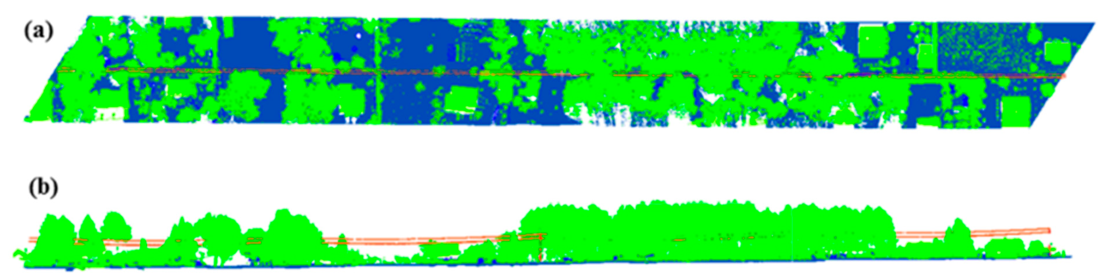
The ALS dataset has been provided by Vimap Olsztyn: the survey has been conducted on 6 July 2017, by means of a RIEGEL VUX1-UAV laser scanner (RIEGL Laser Measurement Systems, Austria), with a helicopter flying at an altitude of approximately 100 m. The fragment of point cloud used in this work contains 2,332,746 points and is shown in Figure 3. The presented ALS point cloud is classified.

As already mentioned, in this case, both OptD and random sub-sampling in CloudCompare were applied in order to reduce the point cloud size at 10% of its original size. The obtained results are shown in

Table 2. Characteristics of the ALS dataset before and after data reduction.

	100%	OptD@10%	CC@10%
The number of data	2,332,746	233,275	233,274
Zmax [m]	108.600	108.600	107.440
Zmin [m]	84.620	84.620	84.980
Zmean [m]	91.634	91.706	89.608
Average point distance [m]	0.036	0.507	0.510

.

Similar to the MLS case, only the OptD method maintained the original values of Z_min and Z_max, whereas the average point distance obtained after applying the two data reduction methods is quite similar.

3. Results

3.1. Light Pole

This subsection aims at evaluating the data reduction effect on light pole points. In this case, three classes of areas are considered: points far from LPs (and from other objects of interest), points under LP, and those appertaining to a LP. The goal of this distinction is analysis of the behavior of the data reduction algorithms, and in particular of the OptD method, in these three cases.

Figure 4 presents the differences in reduction conducted by means of OptD and random sub-sampling implemented in CloudCompare on a fragment of the scanned road. The reduction rate was set to 1% in both cases.

Figure 5 shows the effects of OptD data reduction on LPs and on their surrounding area. As can be seen in Figure 5 (bottom), the behavior of the OptD in the three cases mentioned above is clearly different.

First, OptD sub-samples points with a high data reduction rate in the geometrically regular/smooth areas far from any LP: this is clearly in agreement with the required overall reduction rate and with the general down-sampling behavior of the OptD method, which, roughly speaking, removes points corresponding to redundant information, such as part of the points on planar surfaces.

The OptD behavior on points appertaining to LPs is clearly different from the previous case: thanks to the changes to the original OptD algorithm described in Section 2.2, in this case the data reduction rate is apparently much smaller. Furthermore, by construction, the algorithm also maintains a quite high density of points in the ground area close to the light poles, which can be very important for the implementation of a proper inventory of such objects.

Figure 6 aims at clarifying the advantage of using OptD with respect to a random sub-sampling of the areas close to a light pole: Figure 6a shows the original point cloud, whereas Figure 6b,c show the point cloud reduced at 1% of its original size by means of OptD and random sub-sampling, respectively.

The potential of the proposed OptD method with respect to random sub-sampling shall be apparent when comparing Figure 6b with Figure 6c: few points appertaining to the LP remains in Figure 6c, whereas most of the original ones have been preserved in Figure 6b.

Table 3. Effect of data reduction on points appertaining to a LP.

LP	100%	OptD@1%	CC@1%
	Number of Points
LP 1	5623	2301	51
LP 2	4087	2202	43
LP 3	3978	2235	36

,

Table 4. Effect of data reduction on points in the surrounding area of a LP.

LP	100%	OptD@1%	CC@1%
	Number of Points
LP 1	99,093	5657	834
LP 2	57,753	5833	728
LP 3	50,125	5548	698

and

Table 5. Effect of data reduction on points far from LPs.

LP	100%	OptD@1%	CC@1%
	Number of Points
LP 1	295,635	198	3157
LP 2	346,340	251	3637
LP 3	111,141	85	1029

aim at numerically quantifying the previous considerations in the three classes of areas mentioned above (points appertaining to a LP, to the ground area close to a LP, or far from any of them). Three sample areas have been considered for each of such classes, those shown in Figure 6. Then, the following tables report the numerical results obtained after applying OptD and random sub-sampling on each of these nine sample areas.

The significant data reduction applied to the considered dataset is clearly visible from the results shown in Table 3, where both considered approaches dramatically reduced the number of original points. However, the two methods led to tremendously different results as it seen in Table 4, and quite different as it presented in Table 5. According to the results shown above, LP detection and recognition is probably impossible after applying random sub-sampling at 1% reduction rate. Differently, since OptD method maintained a quite large portion of the LP points, object recognition is still possible in this case.

3.2. Traffic Sign

This subsection considers the effects of data reduction on the traffic sign points. Figure 7 shows the original MLS point cloud considered in this subsection (a) with those sub-sampled by using OptD (b) and with random down-sampling in CloudCompare (c).

Figure 8, Figure 9 and Figure 10 show the data reduction effect (obtained with either OptD or random sub-sampling at 1% of the original point cloud size) on three types of traffic signs: round, triangular, and rectangular. The corresponding numerical results are reported in

Table 6. Effect of data reduction on TS points.

TS	100%	OptD@1%	CC@1%
	Number of Points
TS round	1125	562	16
TS triangle	1334	548	9
TS rectangle	7211	1853	72

.

From the results shown in Table 6, it is quite apparent that the TS points maintained after applying the random sub-sampling at 1% reduction rate are probably insufficient to apply any kind of reasonable TS detection/recognition algorithm. Differently, OptD maintained a much larger portion of the original TS points (50, 41, and 27% for the round, triangular, and rectangular TS case, respectively).

3.3. Power Lines

This subsection deals with the assessment of the data reduction performance in the power line case. Differently from the previous subsections, in this case the analysis is conducted on an ALS dataset, performing data reduction at the 10% of the original point cloud size. Figure 11 shows several fragments of data including some power lines. The original and the sub-sampled point clouds are shown in Figure 11a–c, whereas

Table 7. Effect of data reduction on PL points.

PL	100%	OptD@10%	CC@10%
	Number of Points
PL	4839	4538	285
Terrain points	1,092,951	15,684	121,815
Trees and buildings	1,234,956	213,052	245,025

reports the numerical results concerning the application of the data reduction methods on PL points.

Figure 11 and Table 7 show that most of the PL points have been maintained by the OptD method, whereas the few PL points remaining after random sub-sampling are hardly visible. Interestingly, Table 7 also shows the different behavior of OptD for what concerns ground and trees/building points: the quite high geometric regularity of ground points caused a very high reduction for such category, whereas the data reduction for trees and buildings was less marked.

Since OptD maintained 94% of the PL points, the performance of any successive automatic data processing tool on such points (for instance for PL inventory) is expected to provide qualitative results similar to those on the original dataset. This consideration is also confirmed by the graphical example of Figure 12.

Figure 12a presents the original course of power lines. In Figure 12b, we still observe the points which represent PL, while in Figure 12c after random reduction there are only few points belonging to PL.

3.4. Roadside Trees

The last of the extracted objects were roadside trees. In the first approach, an attempt was made to detect roadside trees from the MLS data. The results are shown in Figure 13.

Roadside trees extraction from the MLS point cloud performed with the use of OptD method allow to obtain satisfactory results. In the

Table 8. Effect of data reduction on RT points.

RT	100%	OptD@1%	CC@1%
	Number of Points
RT	644,839	414,538	366,285

the effect of data reduction on RT points was presented.

Trees are often found as fragments of forests or compact complexes. Thus, it is difficult to extract individual trees without separating the tree into the leaf-off trunk and tree crown. In addition, trees found in clusters have different heights and there is no clear division between the trunk and the crown. The points representing the crowns of the lower trees coincide with the points representing the trunks of the higher trees. Trees are also located at different distances from the road. They are not positioned exactly along the road; therefore, part of the laser beam may be dispersed, reflected from terrain obstacles, etc. However, in this case, it seems that random resampling to some degree enables RT detection.

4. Discussion

Nowadays, LiDAR technology is widely used for collecting data related to transport infrastructures, roads, and on-road/off-road objects. Since several applications require an automatic workflow to extract information of interest from the LiDAR, recent studies considered different approaches in order to automatically detect objects of interest from such datasets. However, the increasing acquisition performance of LiDAR instruments is leading to the availability of surveying systems capable of collecting a huge amount of 3D points in a short time, and consequently, to the necessity of developing computationally efficient strategies to process such very large dataset.

Since the direct application of object detection methods on large raw LiDAR datasets can be computationally inefficient, this paper considered the use of the OptD method as a pre-processing step in order to tremendously reduce the dataset size, while keeping most of the geometric information of interest for the considered application. The rationale is that, since the OptD method is computationally very efficient, if it properly preserves the information about the objects of interest, then it can be used as a pre-processing step in order to significantly speed up the successive object detection phase.

To be more specific, this work focused on the application of OptD in the off-road object detection case. The OptD method was applied on MLS and ALS datasets assessing the suitability of its data reduction for what concerns the detection of three classes of off-road objects: light poles, traffic signs, and power lines. According to the results obtained in the experiments shown in this paper, and summarized in

Table 9. Information about LP preserved after data reduction.

LP	Shape (e.g., Height, Radius etc.)	LP Pole (Height, Diameter, Localization on the Ground)	Object’s Cross Section	Terrain Points	Distance between Following Poles
OptD	√	√	√	√	√
Random sub-sampling	–	–	–	√	√

,

Table 10. Information about TS preserved after data reduction.

TS	Shape and Size (Length, Width, etc.)	TS Pole (Height, Diameter, Localization	Height	Terrain Points
OptD	√	√	√	√
Random sub-sampling	–	–	–	√

and

Table 11. Information about PL preserved after data reduction.

PL	Points Representing PL (Its Course)	Possibility of Fitting the Curve	Measurement of Deflection
OptD	√	√	√
Random sub-sampling	√	–	–

, the OptD can be a suitable method to dramatically reduce the LiDAR dataset size while preserving most of the information needed for the identification of the considered off-road objects, hence enabling a significant speed up of the object detection phase.

As a side effect, since the applied data reduction typically keeps much more points related to the objects of interest than of the others, it may also ease their detection.

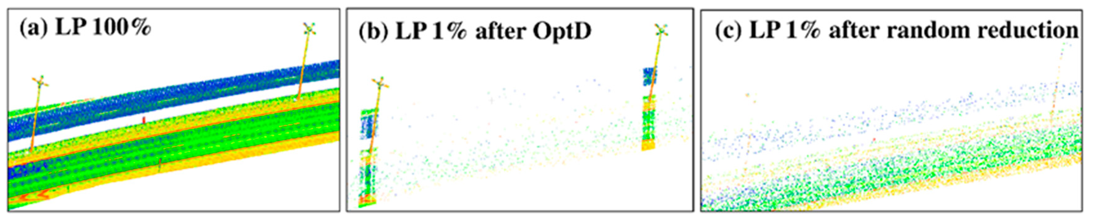
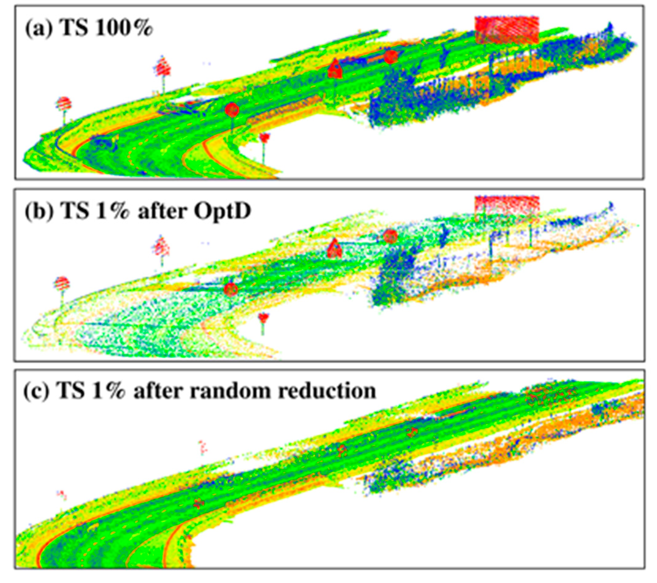
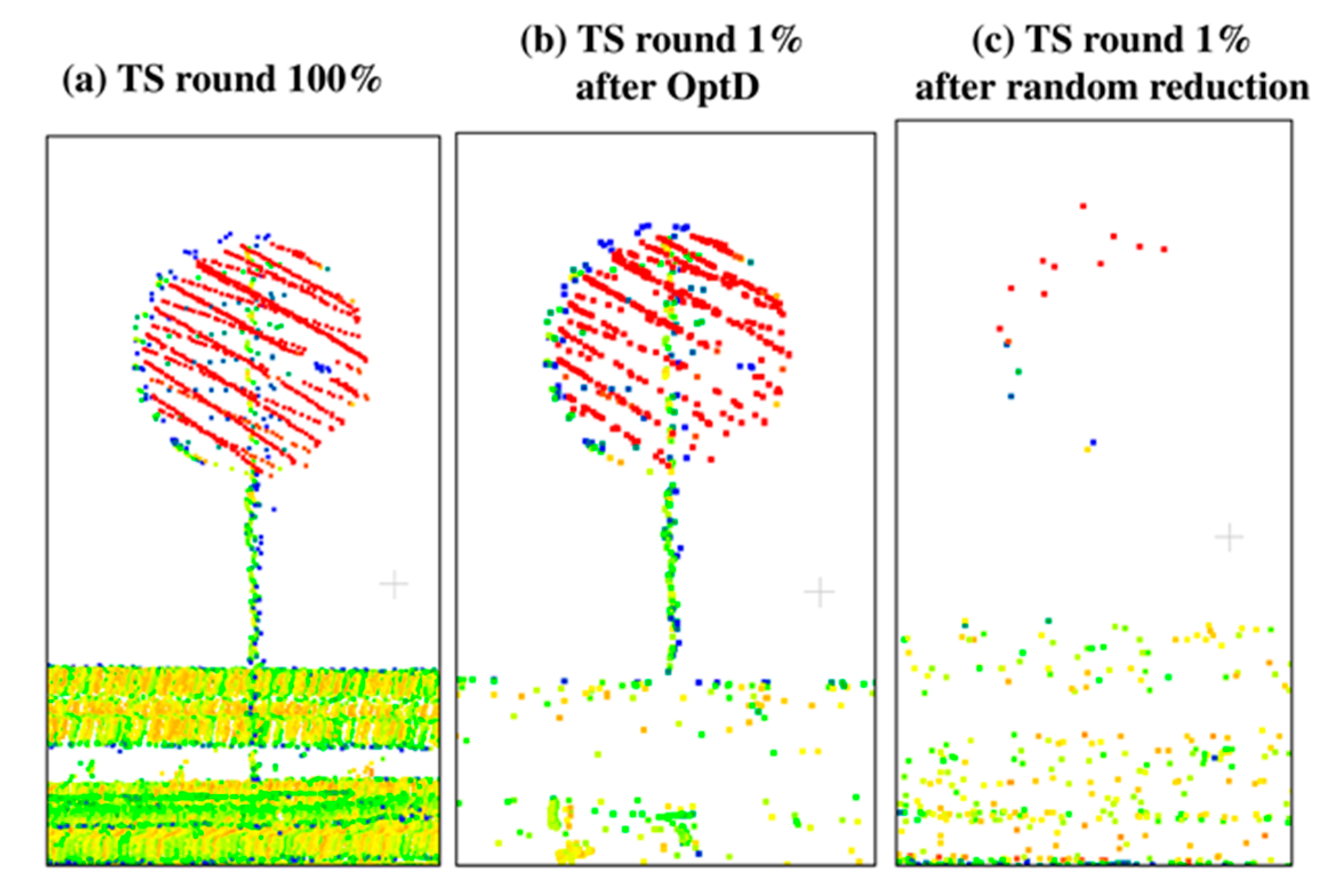
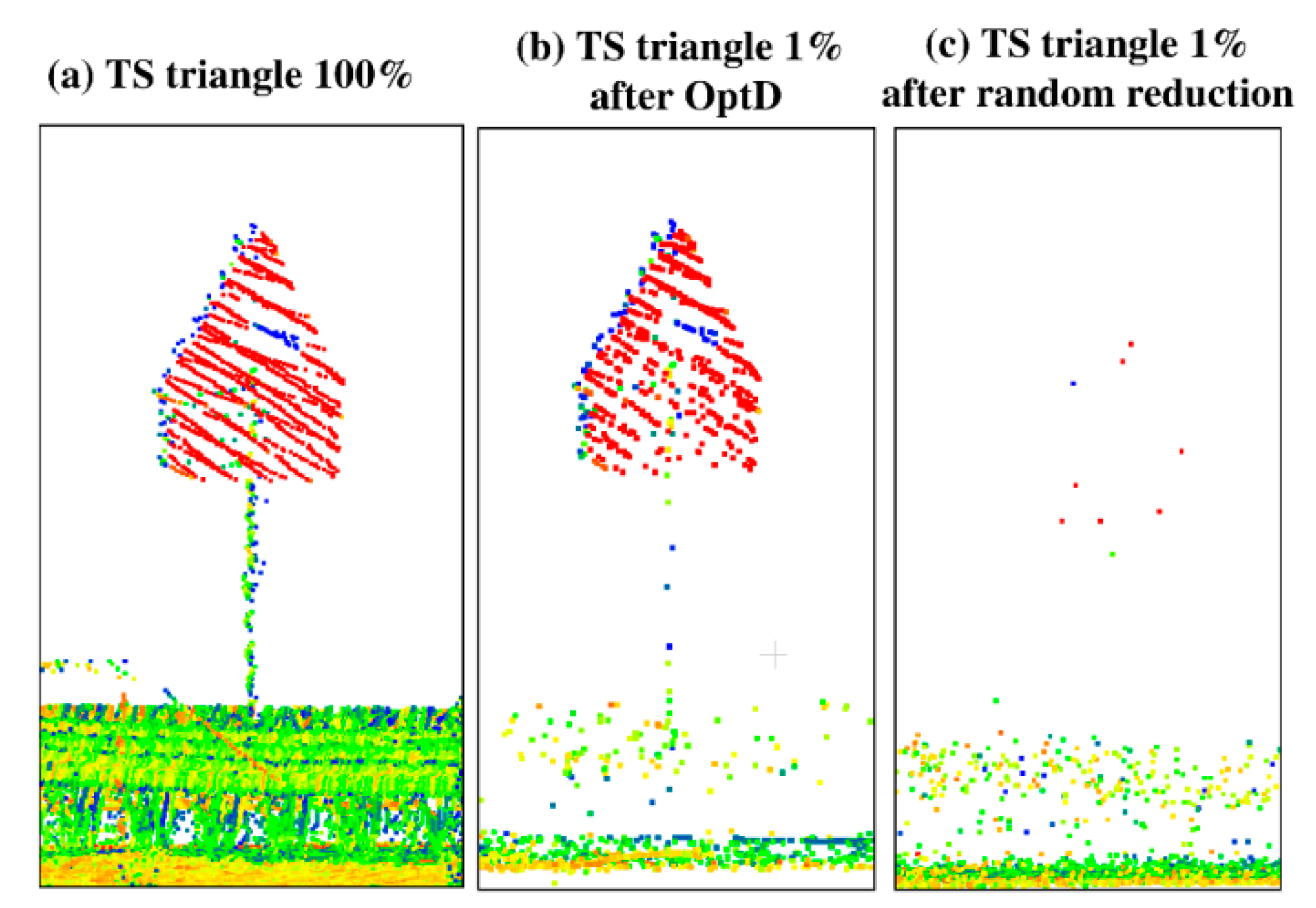
In fact, the proposed method might also be considered a pre-processing step in a much wider range of cases. However, in such case, the proposed data reduction method might cause some issues when dealing with the detection/recognition of objects characterized by very regular surfaces (e.g., planar surfaces), which are those more affected by the OptD data reduction. The obtained results showed that a naïve data reduction based on random sub-sampling the original point cloud typically cannot be used to significantly reduce the dataset size: in this case, the approximately uniform data down-sampling typically causes the loss of most of the information about the off-road objects. Differently, the OptD method applies a non-uniform data reduction, tailored on the geometric characteristics of the dataset and on the specific optimization strategies specified in its implementation (check Section 2.2 for the changes applied here to the previously developed OptD method). The results on the examples reported in Section 3 confirm that the OptD method properly preserves most of the information of interest for off-road object detection in all the considered cases. Table 9, Table 10, and Table 11 summarize the obtained results for what concerns the data reduction in the three considered off-road object classes.

5. Conclusions

In this paper, the OptD method was proposed for the LiDAR data reduction in the framework of off-road object detection. The rationale of the proposed strategy is that of using OptD as a pre-processing step aiming at significantly reducing the size of the dataset to be used as input for a successive object detection algorithm. According to the results of the tests shown in this paper, the following conclusions are now in order:

• OptD method allows a significant reduction of the datasets while preserving most of the information about the off-road objects of interest. In fact, even after a dramatic data reduction of the LiDAR dataset, it is still possible to find enough points of the considered off-road objects in order to properly recognize (model) them, hence, leading to a potentially much more computationally efficient object detection phase.
• Since the OptD data reduction selectively maintains more points about the off-road objects of interest, such a step may also ease/improve their identification phase.
• A consequence of the non-uniform OptD data reduction is that regular surfaces are much more affected by such reduction than by a random sub-sampling, i.e., the OptD method typically maintains a small amount of terrain/ground points.