Sea Level Trend and Fronts in the South Atlantic Ocean


Abstract
1. Introduction
1.1. Untangling Sea Level Trend
1.2. Processes that Affect Sea Level Trend in the South Atlantic
1.3. Scope and Article Organization
2. Materials and Methods
2.1. Sea Level Anomaly
- (1)
- CMEMS: gridded sea level anomaly maps of ¼ of a degree and daily resolution produced and distributed by the Copernicus Marine and Environment Monitoring Service (CMEMS, https://www.marine.copernicus.eu). The delayed time all-sat (DT all-sat) product is used because it is more precise than near real-time data and has the best possible spatial and temporal sampling. In fact, this product was successfully used to study sea level variability in the South West Atlantic (e.g., [18,19,34,35]). The SLA maps are constructed merging all the available satellite missions (TOPEX/POSEIDON, Jason-1, Geosat Follow-on, Jason-2, Envisat, ERS-1, ERS-2, Cryosat-2, Saral/Altika, Jason-3, Sentinel-3A, HY-2A). There are more than three satellites 70 percent of the time, which increase spatial resolution and improve coverage in high latitudes. An optimal interpolation with realistic correlation functions is applied to produce the high spatial resolution SLA maps [36]. To compare this data with the other data sets (see below), we computed a monthly mean for the January 1993 to December 2017 period. In addition, we used gridded Absolute Dynamic Topography (ADT) to analyze the interannual variability of BMC, Subantarctic Front (SAF) and Polar Front (PF). The ADT product is computed as the SLA plus Mean Dynamic Topography (MDT) [37].
- (2)
- CSIRO: the sea level products offered by CSIRO Oceans and Atmosphere, Centre for Southern Hemisphere Oceans. The chosen product is based on satellite altimetry data (www.cmar.csiro.au/sealevel/sl_data_cmar.html). CSIRO delivers gridded global monthly maps of SLA, combining TOPEX/Poseidon, Jason-1, Jason-2/OSTM and Jason-3 with one-degree resolution. The advantage of these missions is that they provide the most accurate long-term stability [38]. Within this product, there are different versions depending on the correction applied, such as IB and GIA (the static terms of SLA). The IB removes the effect of atmospheric pressure on sea level, on scales longer than seasonal and GIA correction removes the effect of vertical crustal motions due to post-glacial rebound. For this study, we downloaded the SLA maps corrected (i) only by IB and (ii) by GIA and IB for the period January 1993 to December 2017.
2.2. Steric Height
2.3. Ocean Mass
3. Results
3.1. Sea Level Trends and Fronts
3.2. What Are the Drivers of SLA Trends in the South Atlantic?
4. Discussion and Conclusions
Author Contributions
Funding
Acknowledgments
Conflicts of Interest
References
- Church, J.A.; White, N.J. Sea-level rise from the late 19th to the early 21st century. Surv. Geophys. 2011, 32, 585–602. [Google Scholar] [CrossRef]
- Cazenave, A.; Palanisamy, H.; Ablain, M. Contemporary sea level changes from satellite altimetry: What have we learned? What are the new challenges? Adv. Space Res. 2018, 62, 1639–1653. [Google Scholar] [CrossRef]
- Merrifield, M.A.; Merrifield, S.T.; Mitchum, G.T. An anomalous recent acceleration of global sea level rise. J. Clim. 2009, 22, 5772–5781. [Google Scholar] [CrossRef]
- Church, J.A.; Clark, P.U.; Cazenave, A.; Gregory, J.M.; Jevrejeva, S.; Levermann, A.; Merrifield, M.A.; Milne, G.A.; Nerem, R.S.; Nunn, P.D.; et al. Sea level change. In Climate Change 2013: The Physical Science Basis. Contribution of Working Group I to the Fifth Assessment Report of the Intergovernmental Panel on Climate Change; Stocker, T.F., Qin, D., Plattner, G.-K., Tignor, M., Allen, S.K., Boschung, J., Nauels, A., Xia, Y., Bex, V., Midgley, P.M., Eds.; Cambridge University Press: Cambridge, UK; New York, NY, USA, 2013. [Google Scholar]
- Ablain, M.; Legeais, J.F.; Prandi, P.; Marcos, M.; Fenoglio-Marc, L.; Dieng, H.B.; Benveniste, J.; Cazenave, A. Satellite altimetry-based sea level at global and regional scales. Surv. Geophys. 2016, 38, 7–31. [Google Scholar] [CrossRef]
- Church, J.A.; White, N.J.; Konikow, L.F.; Domingues, C.; Cogley, J.G.; Rignot, E.; Gregory, J.M.; Broeke, M.V.D.; Monaghan, A.; Velicogna, I. Revisiting the Earth’s sea-level and energy budgets from 1961 to 2008. Geophys. Res. Lett. 2011, 38, 18601. [Google Scholar] [CrossRef]
- Levitus, S.; Antonov, J.I.; Boyer, T.P.; Locarnini, R.A.; Garcia, H.; Mishonov, A.V. Global ocean heat content 1955–2008 in light of recently revealed instrumentation problems. Geophys. Res. Lett. 2009, 36, L07608. [Google Scholar] [CrossRef]
- Rhein, M.; Rintoul, S.R.; Aoki, S.; Campos, E.; Chambers, D.; Feely, R.A.; Gulev, S.; Johnson, G.C.; Josey, S.A.; Kostianoy, A.; et al. Observations: Ocean. In Climate Change 2013: The Physical Science Basis. Contribution of Working Group I to the Fifth Assessment Report of the Intergovernmental Panel on Climate Change; Stocker, T.F., Qin, D., Plattner, G.-K., Tignor, M., Allen, S.K., Boschung, J., Nauels, A., Xia, Y., Bex, V., Midgley, P.M., Eds.; Cambridge University Press: Cambridge, UK; New York, NY, USA, 2013. [Google Scholar]
- Gill, A.; Niller, P. The theory of the seasonal variability in the ocean. Deep Sea Res. Oceanogr. Abstr. 1973, 20, 141–177. [Google Scholar] [CrossRef]
- Steele, M.; Ermold, W. Steric sea level change in the northern seas. J. Clim. 2007, 20, 403–417. [Google Scholar] [CrossRef]
- Dieng, H.B.; Champollion, N.; Cazenave, A.; Wada, Y.; Schrama, E.; Meyssignac, B. Total land water storage change over 2003–2013 estimated from a global mass budget approach. Environ. Res. Lett. 2015, 10, 124010. [Google Scholar] [CrossRef]
- Lambeck, K.; Nakiboglu, S.M. Recent global changes in sea level. Hist. Geophys. 1986, 2, 153–155. [Google Scholar] [CrossRef]
- Peltier, W.R.; Tushingham, A.M. Influence of glacial isostatic adjustment on tide gauge measurements of secular sea level change. J. Geophys. Res. Solid Earth 1991, 96, 6779–6796. [Google Scholar] [CrossRef]
- Stammer, D.; Cazenave, A.; Ponte, R.M.; Tamisiea, M.E. Causes for contemporary regional sea level changes. Annu. Rev. Mar. Sci. 2013, 5, 21–46. [Google Scholar] [CrossRef] [PubMed]
- Qiu, B.; Chen, S. Multidecadal sea level and gyre circulation variability in the northwestern tropical pacific ocean. J. Phys. Oceanogr. 2012, 42, 193–206. [Google Scholar] [CrossRef]
- Qiu, B.; Chen, S.; Wu, L.; Kida, S. Wind- versus eddy-forced regional sea level trends and variability in the north pacific ocean. J. Clim. 2015, 28, 1561–1577. [Google Scholar] [CrossRef]
- Qu, T.; Fukumori, I.; Fine, R.A. Spin-up of the southern hemisphere super gyre. J. Geophys. Res. Oceans 2019, 124, 154–170. [Google Scholar] [CrossRef]
- Etcheverry, L.R.; Saraceno, M.; Piola, A.R.; Strub, P.T. Sea level anomaly on the Patagonian continental shelf: Trends, annual patterns and geostrophic flows. J. Geophys. Res. Oceans 2016, 121, 2733–2754. [Google Scholar] [CrossRef]
- Saraceno, M.; Simionato, C.G.; Ruiz-Etcheverry, L.A. Sea surface height trend and variability at seasonal and interannual time scales in the Southeastern South American continental shelf between 27 S and 40 S. Cont. Shelf Res. 2014, 91, 82–94. [Google Scholar] [CrossRef]
- Ridgway, K.; Dunn, J.R. Observational evidence for a Southern Hemisphere oceanic supergyre. Geophys. Res. Lett. 2007, 34. [Google Scholar] [CrossRef]
- Vianna, M.L.; Menezes, V.V. Double-celled subtropical gyre in the South Atlantic Ocean: Means, trends, and interannual changes. J. Geophys. Res. Space Phys. 2011, 116. [Google Scholar] [CrossRef]
- Artana, C.; Provost, C.; Lellouche, J.; Rio, M.; Ferrari, R.; Sennéchael, N. The Malvinas current at the confluence with the Brazil current: Inferences from 25 years of Mercator ocean reanalysis. J. Geophys. Res. Oceans 2019, 124, 7178–7200. [Google Scholar] [CrossRef]
- Leyba, I.M.; Solman, S.A.; Saraceno, M. Trends in sea surface temperature and air–sea heat fluxes over the South Atlantic Ocean. Clim. Dyn. 2019, 53, 4141–4153. [Google Scholar] [CrossRef]
- Chelton, D.B.; Schlax, M.G.; Witter, D.L.; Richman, J.G. Geosat altimeter observations of the surface circulation of the Southern Ocean. J. Geophys. Res. Space Phys. 1990, 95, 17877. [Google Scholar] [CrossRef]
- Saraceno, M.; Provost, C. On eddy polarity distribution in the southwestern Atlantic. Deep Sea Res. Part I Oceanogr. Res. Pap. 2012, 69, 62–69. [Google Scholar] [CrossRef]
- Leyba, I.M.; Solman, S.A.; Saraceno, M. Air-sea heat fluxes associated to mesoscale eddies in the Southwestern Atlantic Ocean and their dependence on different regional conditions. Clim. Dyn. 2016, 49, 2491–2501. [Google Scholar] [CrossRef]
- Richardson, P. Agulhas leakage into the Atlantic estimated with subsurface floats and surface drifters. Deep Sea Res. Part I Oceanogr. Res. Pap. 2007, 54, 1361–1389. [Google Scholar] [CrossRef]
- Beal, L.M.; Elipot, S. Broadening not strengthening of the Agulhas Current since the early 1990s. Nature 2016, 540, 570–573. [Google Scholar] [CrossRef]
- Backeberg, B.; Penven, P.; Rouault, M. Impact of intensified Indian Ocean winds on mesoscale variability in the Agulhas system. Nat. Clim. Chang. 2012, 2, 608–612. [Google Scholar] [CrossRef]
- Ponte, R.M. Variability in a homogeneous global ocean forced by barometric pressure. Dyn. Atmos. Oceans 1993, 18, 209–234. [Google Scholar] [CrossRef]
- Peltier, W.R. Global glacial isostasy and the surface of the ice-age earth: The ICE-5G (VM2) model and GRACE. Annu. Rev. Earth Planet. Sci. 2004, 32, 111–149. [Google Scholar] [CrossRef]
- Levine, R.A.; Wilks, D.S. Statistical Methods in the Atmospheric Sciences. J. Am. Stat. Assoc. 2000, 95, 344. [Google Scholar] [CrossRef]
- Dieng, H.B.; Cazenave, A.; Meyssignac, B.; Ablain, M. New estimate of the current rate of sea level rise from a sea level budget approach. Geophys. Res. Lett. 2017, 44, 3744–3751. [Google Scholar] [CrossRef]
- Artana, C.I.; Ferrari, R.; Koenig, Z.; Sennéchael, N.; Saraceno, M.; Piola, A.R.; Provost, C. Malvinas current volume transport at 41° S: A 24 yearlong time series consistent with mooring data from 3 decades and satellite altimetry. J. Geophys. Res. Oceans 2018, 123, 378–398. [Google Scholar] [CrossRef]
- Ferrari, R.; Artana, C.I.; Saraceno, M.; Piola, A.R.; Provost, C. Satellite altimetry and current-meter velocities in the Malvinas Current at 41° S: Comparisons and modes of variations. J. Geophys. Res. Oceans 2017, 122, 9572–9590. [Google Scholar] [CrossRef]
- Pujol, M.; Faugère, Y.; Taburet, G.; Dupuy, S.; Pelloquin, C.; Ablain, M.; Picot, N. DUACS DT2014: The new multi-mission altimeter data set reprocessed over 20 years. Ocean Sci. 2016, 12, 1067–1090. [Google Scholar] [CrossRef]
- Mulet, S.; Rio, M.H.; Greiner, E.; Picot, N.; Pascual, A. New Global Mean Dynamic Topography from a GOCE Geoid Model, Altimeter Measurements and Oceanographic In-Situ Data, OSTST Boulder USA. 2013. Available online: http://www.aviso.altimetry.fr/fileadmin/documents/OSTST/2013/oral/mulet_MDT_CNES_CLS13.pdf (accessed on 31 August 2016).
- Ablain, M.; Cazenave, A.; Valladeau, G.; Guinehut, S. A new assessment of the error budget of global mean sea level rate estimated by satellite altimetry over 1993–2008. Ocean Sci. Eur. Geosci. Union 2009, 5, 193–201. [Google Scholar] [CrossRef]
- Masters, D.; Nerem, R.S.; Choe, C.; Leuliette, E.; Beckley, B.; White, N.; Ablain, M. Comparison of global mean sea level time series from TOPEX/Poseidon, Jason-1, and Jason-2. Mar. Geod. 2012, 35, 20–41. [Google Scholar] [CrossRef]
- Escudier, P.; Couhert, A.; Mercier, F.; Mallet, A.; Thibaut, P.; Tran, N.; Amarouche, L.; Picard, B.; Carrere, L.; Dibarboure, G.; et al. Satellite radar altimetry: Principle, accuracy and precision. In Satellite Altimetry Over Oceans and Land Surfaces; Stammer, D.L., Cazenave, A., Eds.; CRC Press, Taylor and Francis Group: Boca Raton, FL, USA, 2018; p. 617. ISBN -13:978-1-4987-4345-7. [Google Scholar]
- Quartly, G.D.; Legeais, J.F.; Ablain, M.; Zawadzki, L.; Fernandes, J.; Rudenko, S.; Carrère, L.; García, P.N.; Cipollini, P.; Andersen, O.B.; et al. A new phase in the production of quality-controlled sea level data. Earth Syst. Sci. Data 2017, 9, 557–572. [Google Scholar] [CrossRef]
- Legeais, J.F.; Ablain, M.; Zawadzki, L.; Zuo, H.; Johannessen, J.A.; Scharffenberg, M.G.; Fenoglio-Marc, L.; Fernandes, J.; Andersen, O.B.; Rudenko, S.; et al. An improved and homogeneous altimeter sea level record from the ESA Climate Change Initiative. Earth Syst. Sci. Data 2018, 10, 281–301. [Google Scholar] [CrossRef]
- Ablain, M.; Meyssignac, B.; Zawadzki, L.; Jugier, R.; Ribes, A.; Cazenave, A.; Picot, N. Error Variance-Covariance Matrix of Global Mean Sea Level Estimated from Satellite Altimetry (TOPEX, Jason 1, Jason 2, Jason 3). Seanoe 2018. [Google Scholar] [CrossRef]
- Ablain, M.; Cazenave, A.; Larnicol, G.; Balmaseda, M.; Cipollini, P.; Faugère, Y.; Fernandes, J.; Henry, O.; Johannessen, J.A.; Knudsen, P.; et al. Improved sea level record over the satellite altimetry era (1993–2010) from the Climate Change Initiative project. Ocean Sci. 2015, 11, 67–82. [Google Scholar] [CrossRef]
- McDougall, T.J.; Barker, P.M. Getting Started with TEOS-10 and the Gibbs Seawater (GSW) Oceanographic Toolbox; SCOR/IAPSO WG: Arnhem, The Netherlands, 2011. [Google Scholar]
- Böning, C.; Willis, J.; Landerer, F.; Nerem, R.S.; Fasullo, J.T. The 2011 La Niña: So strong, the oceans fell. Geophys. Res. Lett. 2012, 39. [Google Scholar] [CrossRef]
- Wahr, J.; Zhong, S. Computations of the viscoelastic response of a 3-D compressible earth to surface loading: An application to glacial isostatic adjustment in Antarctica and Canada. Geophys. J. Int. 2012, 192, 557–572. [Google Scholar] [CrossRef]
- Chambers, D.P.; Bonin, J.A. Evaluation of release 05 time-variable gravity coefficients over the ocean. Ocean Sci. 2012, 8, 859–868. [Google Scholar] [CrossRef]
- Sakumura, C.; Bettadpur, S.; Bruinsma, S. Ensemble prediction and intercomparison analysis of GRACE time-variable gravity field models. Geophys. Res. Lett. 2014, 41, 1389–1397. [Google Scholar] [CrossRef]
- Cazenave, A. WCRP global sea level budget group: Global sea-level budget 1993–present. Earth Syst. Sci. Data 2018, 10, 1551–1590. [Google Scholar] [CrossRef]
- Dieng, H.B.; Cazenave, A.; Von Schuckmann, K.; Ablain, M.; Meyssignac, B. Sea level budget over 2005–2013: Missing contributions and data errors. Ocean Sci. 2015, 11, 789–802. [Google Scholar] [CrossRef]
- Royston, S.; Vishwakarma, B.D.; Westaway, R.; Rougier, J.; Sha, Z.; Bamber, J. Can we resolve the basin-scale sea level trend budget from GRACE ocean mass? J. Geophys. Res. Oceans 2020, 125, e2019JC015535. [Google Scholar] [CrossRef]
- Mason, E.; Pascual, A.; Gaube, P.; Ruiz, S.; Pelegrí, J.L.; Delepoulle, A. Subregional characterization of mesoscale eddies across the Brazil-Malvinas Confluence. J. Geophys. Res. Oceans 2017, 122, 3329–3357. [Google Scholar] [CrossRef]
- Goni, G.J.; Bringas, F.; DiNezio, P.N. Observed low frequency variability of the Brazil Current front. J. Geophys. Res. Space Phys. 2011, 116. [Google Scholar] [CrossRef]
- Saraceno, M.; Valla, D.; Pelegrí, J.L.; Piola, A.R. Seasonal and interannual variability of the Brazil-Malvinas front: An altimetry perspective. In American Geophysical Union, Ocean Sciences Meeting 2016, abstract# PO14E-2865; American Geophysical Union: Washington, DC, USA, 2016. [Google Scholar]
- Gille, S.T. Decadal-scale temperature trends in the Southern Hemisphere Ocean. J. Clim. 2008, 21, 4749–4765. [Google Scholar] [CrossRef]
- Chambers, D.P.; Cazenave, A.; Champollion, N.; Dieng, H.; LloveL, W.; Forsberg, R.; Von Schuckmann, K.; Wada, Y. Evaluation of the global mean sea level budget between 1993 and 2014. Surv. Geophys. 2016, 38, 309–327. [Google Scholar] [CrossRef]
- Roemmich, D.; Gilson, J. The 2004–2008 mean and annual cycle of temperature, salinity, and steric height in the global ocean from the Argo Program. Prog. Oceanogr. 2009, 82, 81–100. [Google Scholar] [CrossRef]
- Tapley, B.D.; Watkins, M.M.; Flechtner, F.; Reigber, C.; Bettadpur, S.; Rodell, M.; Sasgen, I.; Famiglietti, J.; Landerer, F.; Chambers, D.P.; et al. Contributions of GRACE to understanding climate change. Nat. Clim. Chang. 2019, 9, 358–369. [Google Scholar] [CrossRef]
- Ablaini, M.; Meyssignac, B.; Zawadzki, L.; Jugier, R.; Ribes, A.; Spada, G.; Benveniste, J.; Cazenave, A.; Picot, N. Uncertainty in satellite estimates of global mean sea-level changes, trend and acceleration. Earth Syst. Sci. Data 2019, 11, 1189–1202. [Google Scholar] [CrossRef]
- Durack, P.; Wijffels, S.E. Fifty-Year trends in global ocean salinities and their relationship to broad-scale warming. J. Clim. 2010, 23, 4342–4362. [Google Scholar] [CrossRef]
- Roemmich, D.; Gilson, J.; Davis, R.; Sutton, P.; Wijffels, S.; Riser, S. Decadal spinup of the South Pacific subtropical gyre. J. Phys. Oceanogr. 2007, 37, 162–173. [Google Scholar] [CrossRef]


| ADT | BMC/45° W | 40° W–20° W | 20° W–0° E | 0° E–15° E |
|---|---|---|---|---|
| 30 cm | −0.06 °/yr/-- | −0.05 °/yr | −0.12 °/yr | −0.07 °/yr |
| 5 cm (SAF) | --/−0.16 °/yr | −0.06 °/yr | −0.04 °/yr | −0.04 °/yr |
| −40 cm (PF) | --/−0.02 °/yr | −0.03 °/yr | −0.04 °/yr | −0.03 °/yr |
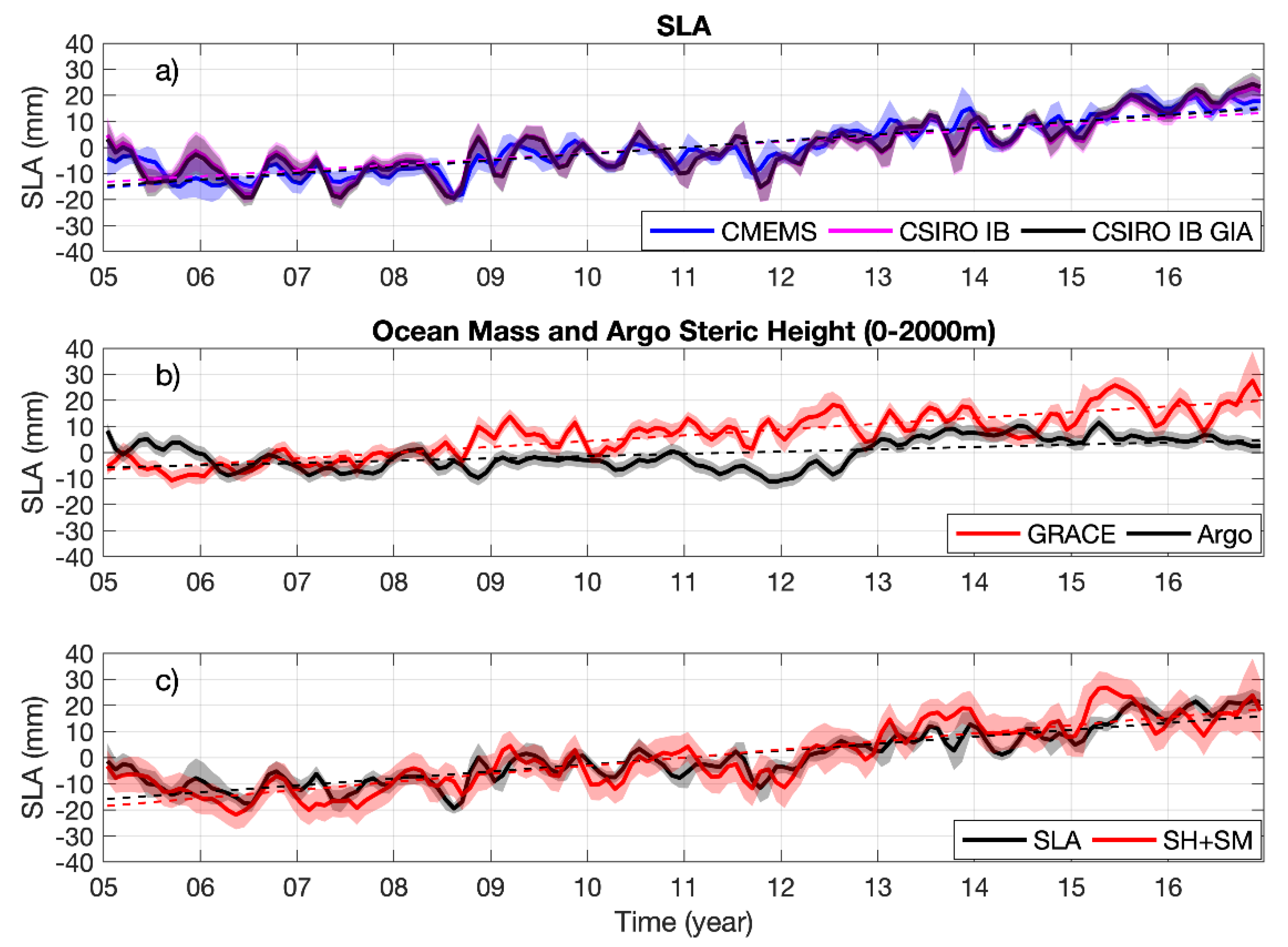
| SAMSL Trend | Non-seasonal SAMSL Trend | |
|---|---|---|
| CMEMS | 2.38 ± 0.59 mm/yr | 2.56 ± 0.36 mm/yr |
| CSIRO IB | 2.02 ± 0.61 mm/yr | 2.21 ± 0.29 mm/yr |
| CSIRO IB GIA | 2.28 ± 0.61 mm/yr | 2.47 ± 0.29 mm/yr |
| GRACE | 2.32 ± 0.45 mm/yr | 2.22 ± 0.21 mm/yr |
| Steric height | 0.50 ± 1.00 mm/yr | 0.88 ± 0.23 mm/yr |
| Thermosteric height | 1.02 ± 1.00 mm/yr | 1.39 ± 0.32 mm/yr |
| Halosteric height | −0.26 ± 0.14 mm/yr | −0.26 ± 0.13 mm/yr |
| GRACE + Steric | 2.81 ± 0.80 mm/yr | 3.10 ± 0.29 mm/yr |
© 2020 by the authors. Licensee MDPI, Basel, Switzerland. This article is an open access article distributed under the terms and conditions of the Creative Commons Attribution (CC BY) license (http://creativecommons.org/licenses/by/4.0/).
Share and Cite
Ruiz-Etcheverry, L.A.; Saraceno, M. Sea Level Trend and Fronts in the South Atlantic Ocean. Geosciences 2020, 10, 218. https://doi.org/10.3390/geosciences10060218
Ruiz-Etcheverry LA, Saraceno M. Sea Level Trend and Fronts in the South Atlantic Ocean. Geosciences. 2020; 10(6):218. https://doi.org/10.3390/geosciences10060218
Chicago/Turabian StyleRuiz-Etcheverry, Laura A., and Martin Saraceno. 2020. "Sea Level Trend and Fronts in the South Atlantic Ocean" Geosciences 10, no. 6: 218. https://doi.org/10.3390/geosciences10060218
APA StyleRuiz-Etcheverry, L. A., & Saraceno, M. (2020). Sea Level Trend and Fronts in the South Atlantic Ocean. Geosciences, 10(6), 218. https://doi.org/10.3390/geosciences10060218