Abstract
This paper describes the implementation and use of a mechanical cone penetration test (CPTm) database for the evaluation of the liquefaction potential in some areas of Tuscany. More specifically, the database contains 4500 CPTm covering an area of 1787 square km and mainly concerns some coastal areas of Tuscany. Available simplified liquefaction evaluation procedures (LEPs) are mainly based on piezocone CPT (CPTu) test results and not on CPTm. An early interest on developing LEPs with reference to CPTm became quite soon obsolete because of the widespread use of piezocone. Unfortunately, in Italy, the use of CPTm is very popular. After the 2012 seismic sequence of Emilia-Romagna, the use of CPTm for liquefaction risk analysis has seen a renewed interest, even though such a topic should require further studies. This paper shows an empirical approach for liquefaction triggering assessment by CPTm using existing LEPs, thus making possible the use of the developed CPTm database for the preliminary screening of the study area.
1. Introduction
Liquefaction occurs mainly in loose saturated sandy soils and is responsible for the total or partial loss of soil resistance [1]. Effects of liquefaction on the urban context can be summarized as follows:
- structures resting on a liquefied soil could suffer relevant differential settlements, tilting, or overturning;
- buried structures are subject to hydraulic heave;
- in free-field conditions, pore water pressure increase and ejecta of sand could damage lifeline systems and several infrastructures;
- instabilities of both natural and artificial slopes can be triggered.
Recent examples of these effects include damage produced during the Emilia-Romagna and Canterbury earthquakes [2,3,4,5,6,7,8,9,10,11,12,13].
Identification of liquefaction prone areas, therefore, has become an important task as national/regional authorities need to define recommendations for sustainable development, land use planning, mitigation of liquefaction, and ground improvement purposes.
The technical literature is rich in contributions about liquefaction evaluation procedures (LEPs), and most of them are simplified empirical procedures [14,15,16,17,18,19,20,21,22,23,24].
LEPs enable one to determine the factor of safety against liquefaction (FSL) at each investigated depth of the soil profile. The FSL is inferred by the ratio between the cyclic resistance ratio (CRR) and the cyclic stress ratio (CSR), which represent the shear strength of the soil and the earthquake-induced shear stress, respectively. Sampling in sandy deposits is very difficult, time consuming, and costly. Therefore, CRR is inferred from in situ tests, typically Standard Penetration Test SPT [14,15,17], cone penetration test (CPT) [18,19,22,23,24,25,26], shear wave velocity [27,28], self-boring pressuremeter test (SBPT) [29], and flat dilatometer test (DMT) [30,31]. The CSR, which represents the amplitude of the seismic demand, is generally assessed via simplified formulations defined in the LEPs.
Once FSL has been evaluated at different depths, an index assessing the effects of liquefaction in terms of damage severity at ground level should be selected and then used for defining liquefaction hazard maps.
The most commonly used severity indexes are the Liquefaction Potential Index (LPI) (Iwasaki et al. [32]) and the Liquefaction Severity Number (LSN) (Tonkin and Taylor [33]). A modification of the LPI was proposed by Sonmez [34]. Papathanassiou et al. [3] have suggested different thresholds for the LPI. The Papathanassiou et al. [3] suggestion is very interesting as it is based on the liquefaction phenomena that occurred during the 2012 Emilia-Romagna sequence. Moreover, specific threshold values of the liquefaction severity in terms of LPI or LSN for each considered LEP and soil characteristics were suggested in Maurer et al. [12]. In any case, the use of different criteria or thresholds or the definition of different thresholds makes sense only when facing a post-liquefaction situation. Therefore, we decided to remain with Iwasaki’s [32] original criteria. The aim was a preliminary screening of the study area and the applicability of the considered LEPs and CPTm database.
In this work, the acronym CPTu indicates a static penetration test that has been carried out using a piezocone (i.e., tip resistance qc, sleeve friction fs, and pore pressure u2 are measured every 1 or 2 cm of penetration). Additionally, the acronym CPTm indicates a static penetration test that has been carried out using a mechanical tip (also called Begemann-type tip in this paper), which provides qc and fs every 20 cm [35]. CPT-based LEPs were developed with reference to CPTu tests. However, in many countries, huge CPTm databases are available. Therefore, it has become important to develop specific procedures enhancing the liquefaction potential evaluation and soil profile reconstruction via existing CPTm databases.
CPTm in comparison to CPTu is affected by a lower resolution, as CPTm measurements (qc and fs) and CPTu measurements (qc, fs, and u2) are available every 20 and 2 (or 1) cm, respectively. This results in difficulties, in the case of CPTm, in identifying very thin liquefiable layers as shown in [22,23] and in Boulanger and DeJong [36]. Moreover, CPTu allows users to measure excess pore pressure during the cone penetration, which is relevant for evaluating the total tip resistance (qt) and improving the capability of correctly identifying the soil behavior type (SBT) [37]. It is also possible to identify the normalized soil behavior type (SBTn), which is especially recommended at greater depths [35,38,39].
Because of the constructive details, the sleeve friction (fs) measured by using the Begemann cone (CPTm) is systematically greater than that obtained with the piezocone (see, as an example, Lo Presti et al. [30]). As both fs and qc are used to identify the SBT (or SBTn), it is obvious that differences in terms of fs and qc could affect the assessment of the FSL. On the other hand, while differences in terms of fs are measurable, those in terms of qc are quite negligible [40].
Finally, the interpretation of CPTm tests using the SBTn classification system [16,38] and its soil classification index (IC), which was developed with reference to CPTu, tends to underestimate the grain size (for more details, see Section 4.3). Consequently, loose sands could be erroneously identified as silt mixtures [41,42,43], which in turn leads to an overestimation of the safety factor against liquefaction, FSL. Indeed, the presence of fines leads to an increase in the soil resistance according to the available LEPs.
In various countries, as in Italy, CPT tests are carried out with a mechanical tip. Therefore, CPTm results and CPT-based procedures require some corrections.
In this work, a CPTm database of the Tuscany region (Italy) was implemented and then used to assess the liquefaction hazard of this region’s coastal area. The use of the developed database was possible by applying two recently proposed correction procedures (described in Section 4.3) to re-interpret CPTm results [41,42]. The first correction procedure is based on a correlation between fs measured with CPTm and that obtained from CPTu. Such a correlation was obtained by comparing some pairs of CPTu and CPTm that were carried out in the Pisa plain (Tuscany, Italy). In any case, it is worthwhile to remember that the considered stratigraphy involves both sand, clay, and silt mixture layers. The second correction procedure modifies IC as obtained from CPTm. The correction factor of the classification index (ΔIC) is a function of the measured cone tip resistance (qc).
Such a correlation was obtained by using 78 pairs of CPTm and CPTu that were carried out in the urban areas of San Carlo, Mirabello, and Sant’Agostino, located in the Emilia-Romagna region (Italy) and hit by the 2012 Emilia-Romagna seismic sequence.
The same approach (i.e., the use of a correction factor of the classification index) was used in the case of dredged sediments and silt mixtures [43]. The Emilia-Romagna database and that of Tuscany mainly concern Holocene alluvial deposits of silt mixtures and sandy layers.
In Meisina et al. [41,42], the two correlations were applied to several pairs of CPTm and CPTu tests belonging to the database of the Emilia-Romagna region, which was concerned by the seismic sequence of May–June 2012 (Regione Emilia Romagna [44]), and to some pairs of CPTm and CPTu in a test site located in Pisa.
The above-mentioned papers qualitatively demonstrated the enhanced capability of the re-interpreted CPTm results in identifying the soil profile and the potentially liquefiable layers. Such an assessment of the effectiveness of the adopted correction procedures of CPTm was possible due to the availability of borehole logs and evidence of liquefaction. Moreover, the effectiveness of these correlations in improving the evaluation of the liquefaction severity indexes by CPTm was verified by comparing several pairs of CPTm and CPTu that were carried out in the Emilia-Romagna region. The comparison involved both sites in which liquefaction occurred and sites in which liquefaction did not occur. The predicted liquefaction hazard was consistent with liquefaction phenomena that were observed in 2012. In any case, because of the limited number of CPTu-CPTm pairs, a statistical comparison was not possible.
2. Implementation of the CPT Database of the Tuscany Region
In agreement with the technical staff of the Tuscany region, a plan was drawn up to collect the available CPTm and CPTu tests. The following databases were used:
- CPT test database from the Tuscany region (managed by the consortium LaMMA), and available on [45];
- CPT test database available from the seismic microzonation studies of the municipalities of the Tuscany region;
- CPT test database from the provinces of the Tuscany region.
Furthermore, the Tuscany region and the Department of Civil and Industrial Engineering of Pisa University have recovered further cone penetration tests from engineers and geologists working in this territory. However, it was not possible to find boreholes and undisturbed sampling close to each cone penetration test. Since the groundwater table (GWT) level was rarely available in the CPT test reports, the Tuscany region carried out an ad-hoc study to infer the water table depth from the piezometric surface, which was available for almost the entire study area. The latter was inferred by the phreatimetric studies carried out by the Basin Authorities of the Arno and Serchio rivers (Figure 1). It is important to stress that the water table depth in the whole study area was accurately identified. Indeed, water table is an important parameter. The considered values represent the average depth after considering the seasonal variations. Considering that the seismic risk in Italy is assessed by a probabilistic approach (NTC, 2018 [46]), the average value of the water table depth seems an acceptable assumption for a study covering an area of about 1800 square km. Most of the CPT data were not in a digital format or on a digital support, thus it was necessary to digitize the collected data. The above-mentioned databases consisted of 5362 CPTs. It was possible to convert only 4500 CPTm and 16 CPTu to a digital format. These data represent the available geo-referenced database. Table 1, Table 2 and Table 3 summarize, for each macro-area in which the study territory was divided, the number of available CPT tests (CPTm and CPTu), and the maximum depth attained during the tests.
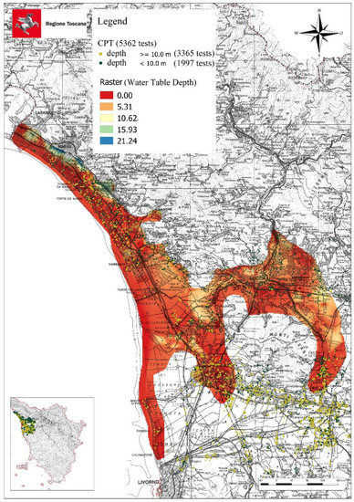
Figure 1.
Map of the piezometric surface in the study area (estimated).

Table 1.
Cone penetration test (CPT) database for the macro-area of Versilia.
Table 2.
CPT database for the macro-area of the Pisa plain.
Table 3.
CPT database for the macro-area of the Lucca plain.
Most of the CPTs were performed in the Pisa plain macro-area (77%, equal to 3456 CPTs), and about half of these tests (49%) fall within the maximum-depth interval of 8–10 m. Only a small number of CPTs (6%) reached depths greater than 20 m. The number of CPTs in the Versilia macro-area represents 17% (equal to 782 CPTs) of the total number, and 31% of these tests fall within the maximum-depth interval of 5–8 m. CPTs available in the Lucca plain are 6% (equal to 278 CPT) of the entire database. Of these tests, 40% reached a maximum-depth interval of 5–8 m and only 3% were in the interval of 15–20 m. Thus, most of the available tests did not exceed the depth of 20 m. As can be easily observed in Table 1, Table 2 and Table 3, almost the entire database is based on cone penetration tests with a mechanical tip (CPTm).
3. Main Geological Features and Historical Liquefaction of the Study Area
From a geological point of view, the study area may be divided into two main sectors—the coastal area of the Pisa plain and Versilia and the innermost zone corresponding to the Lucca plain.
The Lucca plain consists of Quaternary alluvial deposits of the Serchio River. These deposits consist mainly of coarse materials (sands and gravels) at the base, while sands with fines (clay and silts) are found at the top. The alluvial deposits overlay a Pliocene, lacustrine clayey horizon [45]. The risk of liquefaction obviously concerns mainly the shallower layers of silt and sand.
On the other hand, the coastal area of the Pisa plain and Versilia consists of very thick Quaternary (mainly Holocene) alluvial deposits of the Arno, Serchio, and other minor rivers. These deposits are granular at the base and cohesive at the top. Alluvial deposits overlay the coastal marine horizons (marine clays). In the area closest to the coastal line, there are also deposits of aeolian sands of limited thickness and extension [45]. From a geological point of view, only Aeolian sands are different with respect to the considered deposits of the Emilia-Romagna region.
Figure 2 shows those areas that are potentially prone to liquefaction. Liquefaction susceptibility is based on geological criteria. The figure distinguishes those areas that in the last 2000 years have been shocked by earthquakes of Intensity VII and VIII of the Mercalli–Cancani–Sieberg (MCS) intensity scale. The dots locate those sites with evidence of liquefaction as reported by Galli and Meloni [47]. The earthquakes that probably caused liquefaction-related phenomena in Tuscany amount essentially to five and occurred in the period between 1542 and 1919 [47]. It is also worth mentioning that, after the Second World War, the study area experienced a remarkable urbanization. Therefore, the major concern is related to recently urbanized areas.
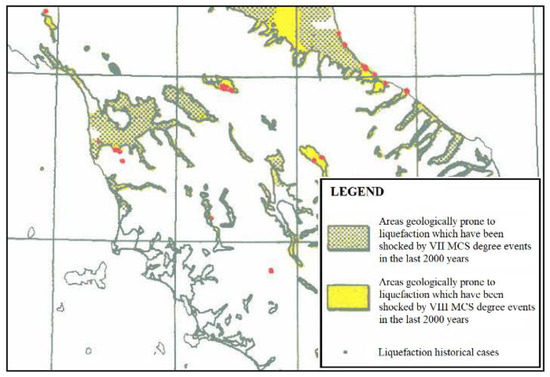
Figure 2.
Areas geologically prone to liquefaction in the study area (adapted from Galli and Meloni [47]).
4. CPT-Based Assessment of Liquefaction Hazard
In this study, the assessment of the Tuscany region’s liquefaction hazard was carried out by using CPT-based LEPs to calculate the factor of safety against liquefaction (FSL) within an LPI framework. The factor of safety was inferred by using the ratio between the cyclic resistance ratio (CRR) and the cyclic stress ratio (CSR) and applying the overburden correction factor (Kσ) and the magnitude scaling factor (MSF). The CSR, which represents the seismic demand, is computed according to Equation (1) [1]:
where σv and are the total and effective geostatic stress, respectively; as is the free-field peak ground acceleration at the ground surface of the site of interest; g is the gravity; and rd is a stress reduction factor accounting for the distribution along depth of the shear stress amplitude (soil flexibility). On the whole, both as and rd should be inferred from site-specific true nonlinear seismic response analysis, accounting for soil strength [48,49,50]. This is difficult in the case of liquefiable deposits and out of the scope of the present paper. Therefore, in this work, as was evaluated at each site following the Italian Building Code [46]. The Italian Building Code provides site-dependent parameters at the nodes of a squared grid of 0.05° size, which covers the entire Italian territory, to define the seismic hazard for each prescribed exceedance probability within a reference period, and thus for each return period. These parameters are as follows: ag, F0, and TC* and represent the maximum free-field acceleration for a rigid reference site with horizontal topographical surface, the maximum spectral amplification factor, and the period above which the spectral velocity is constant, respectively. The as value for a given return period is then obtained as the product of ag and the amplification factors SS and ST, accounting for the stratigraphy and the topography of the considered site. In particular, the SS amplification factor depends on the ground type, thus on the average shear wave velocity of the first 30 m. In other words, the peak ground acceleration was evaluated on the basis of a probabilistic approach including all scenarios. Moreover, for the present study, three different LEPs were used, as more clearly specified later on. The Boulanger and Idriss [24] and the Juang et al. [19] approaches were applied exactly according to their original formulation. For these methods, the stress reduction factor rd was computed according to Equations (2) to (4) [21], in which MW is the earthquake moment magnitude. The Robertson and Wride [16] method does not clearly define the Kσ, MSF, and rd factors. Indeed, Robertson and Wride [16] suggest, according to Youd et al. [17], to use the rd factor defined by Liao and Whitman [51] and the MSF according to the range suggested by Youd et al. [17]. No indication is given as for the Kσ factor. Therefore, for this method, we decided to use the same factors as for the Boulanger and Idriss [24] LEP. Of course, such an assumption could be questionable.
The LPI is used as an index of the potential damage at the soil surface level and was computed according to the original formulation proposed by Iwasaki et al. [32] (Equation (5)):
where F1 = 1 − FSL for FSL ≤ 1 and F1 = 0 for FSL > 1; W(z) is a depth weighting function given by W(z) = 10 − 0.5z; and z is the depth in meters below the ground surface. The LPI can range thus from 0 to a maximum of 100 (i.e., where FSL is zero over the entire 20 m depth). The level of liquefaction severity can be defined according to the categories suggested by Sonmez [34] or by Iwasaki et al. [32]. In this work, the categories defined in [32] are considered, which assumes for LPI = 0 that a site is not likely to liquefy and for 0 < LPI < 5, 5 < LPI < 15, and LPI > 15 there is a low, high, and very high liquefaction severity, respectively.
4.1. Definition of the Seismic Demand
For the definition of the seismic demand, a reference period (VR) of 50 years was considered, and assuming an exceedance probability (pL) of 10% in the reference period, a return period (TR) of 475 years is obtained using Equation (6) [46]:
The amplification factor ST was assumed equal to 1, thus considering the topographic area as flat. The factor SS was inferred from the Italian Building Code [46], assuming a ground type C, which means a stratigraphic profile characterized by an average shear wave velocity of the first 30 m between 180 and 360 m/s. Table 4 shows the values of the free-field peak ground acceleration (as) at each municipality considered in this study. The moment magnitude MW (necessary for determining the magnitude scaling factor (MSF)) was first determined by the disaggregation of the seismic hazard for a return period of 475 years [52]. For all the municipalities in the study area, the modal values of MW (from disaggregation) are between 4.5 and 5.0 (Figure 3). On the other hand, the average values of MW (Figure 4) for some municipalities are between 4.5 and 5.0, while for others they were between 5.0 and 5.5. For simplicity, it was decided to use a unique value, MW = 5.5 (corresponding to the upper limit), for all the municipalities of the study area. From a theoretical point of view, the assumption of a unique value of magnitude means considering a single-scenario earthquake. From a practical point of view, such an assumption is responsible, in some municipalities, for a negligible underestimation of the safety factor (less than 8%). It is worth mentioning that the moment magnitude affects the MSF. Indeed, the earthquake duration (i.e., the number of cycles of equivalent amplitude) increases with the magnitude, which in turn influences the CRR (i.e., the factor of safety against liquefaction). The factor of safety increases as magnitude (MW) decreases.
Table 4.
Free-field peak ground acceleration (as) at each municipality, according to NTC (2018) [46].
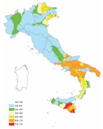
Figure 3.
Modal values of MW from disaggregation [52].
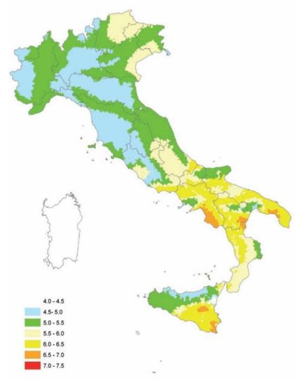
Figure 4.
Average values of MW from disaggregation [52].
4.2. Considered Liquefaction Evaluation Procedures (LEPs)
This section summarizes the adopted LEPs according to their original definition in order to avoid the mix-up of different approaches. CRR was determined according to the Robertson and Wride [16], Boulanger and Idriss [24], and Juang et al. [19] approaches. The approach proposed by Robertson and Wride [16] computes CRR by using Equations (7) and (8):
where qc1N,cs is the normalized tip resistance corrected to account for the overburden stress and the fine content (FC) and is computed using Equations (9) and (10):
where patm is the atmospheric pressure, qc is the measured tip resistance; the n exponent is assumed equal to 1.0 for clayey soil, 0.5 for sandy soil, and 0.75 for silt mixtures; and KC is a correction factor that is computed through Equations (11) and (12):
where IC is the soil classification index as defined by Robertson and Wride [16] (Equations (13)–(15)):
where fs is the measured sleeve friction.
In the procedure developed by Boulanger and Idriss [24], CRR is computed by using Equation (16):
where C0 (=2.6 ± 0.2) is a fitting parameter and qc1N,cs is defined by Equation (17), which requires an iterative procedure by using Equations (18) to (22):
where CFC is a fitting parameter (see Boulanger and Idriss [24] for the suggested value) and IC can be computed using Equation (13) or according to Robertson [38].
In the case of the Boulanger and Idriss [24] and Robertson and Wride [16] approaches, the overburden correction factor (Kσ) is computed by using Equations (23) and (24), whereas the MSF is computed by using Equations (25) and (26):
In the approach proposed by Juang et al. [19], CRR is computed by using Equation (27) in the case of a deterministic liquefaction evaluation:
where qc1N,m (Equation (28)) is the stress-normalized tip resistance qc1N (Equation (18)) adjusted for the fine effect. In the Juang et al. [19] LEP, qc1N is computed via an iterative procedure involving Equations (18) to (20). Please note that, in Equation (20), the term qc1N,cs is replaced by the term qc1N:
In Equation (28), the adjustment factor, K, is part of the regression model shown in Juang et al. [19] and is obtained from Equations (29) to (31):
According to Juang et al. [19], IC is defined in a slightly different way as compared to that defined by Robertson and Wride [16]:
The factor Kσ is computed again with Equation (23); nevertheless, Cσ is defined by Equation (33):
The magnitude scaling factor (MSF) is then obtained through Equation (34) as suggested by Idriss and Boulanger [22]:
Finally, for all the above described LEPs, the factor of safety against liquefaction (FSL) is computed with Equation (35):
When using CPTm results in conjunction with the above summarized LEPs, some corrections to measured fs and estimated IC become mandatory, according to the suggestions provided in the works of Meisina et al. [41,42] and briefly described in Section 4.3. These corrections are independent from each other.
4.3. CPTm Correction Procedure
The correction procedure for using CPTm results together with available LEPs consists of two empirical correlations [41,42]:
- the first correlation is between fs measured with CPTm and that obtained from CPTu;
- the second correlation is between the correction factor (ΔIC) and the cone tip resistance (qc), which is applied in the case of silt mixtures that are non-correctly identified by the SBTn classification system.
In Meisina et al. [41,42], these two correlations were developed and applied to several pairs (92 pairs in total) of CPTm and CPTu tests to verify their effectiveness in enhancing the identification of liquefiable layers and the evaluation of liquefaction severity by CPTm. The developed approach consists of correcting the sleeve friction (fs) measured with CPTm and of modifying the estimated value of the soil classification index (IC) as obtained by interpreting the CPTm data.
The corrected value of IC is only used for improving the soil classification (SBTn), thus it is not applied to Equations (11), (12), (22), and (29)–(31) in which the uncorrected value is still considered. In fact, the use of the SBTn classification system [16,38,39], which is based on CPTu, for the interpretation of CPTm leads on several occasions to an underestimation of the soil grain size, which in turn means an overestimation of IC.
The IC correction is only intended to improve the identification of potentially liquefiable layers, i.e., those layers having an IC less than the IC cut-off value. The latter value (IC cut-off) is used to screen out clay-like soils and is commonly taken between 2.4 and 2.6 [24]. It is worthwhile to remember that those layers with IC higher than IC cut-off are assumed to be non-liquefiable, thus are not considered in the computation of the LPI.
4.3.1. Sleeve Friction (fs) Correction
Meisina et al. [41] compared the sleeve friction from CPTm, fs(CPTm), and that from CPTu, fs(CPTu), as obtained from pairs of adjacent CPTm-CPTu tests. These tests were carried out at a site in Pisa (central Italy). At the Pisa site, a total of 12 penetration tests (3 CPTm and 9 CPTu) were carried out using a Pagani TG 73/200 penetrometer (Pagani Geotechnical Equipment, Piacenza, Italy) [53]. The capabilities of these tests in identifying the soil layering were also verified due to the availability of three continuous boreholes. The soil stratigraphy at the test site in Pisa is very similar to that existing beneath the Leaning Tower of Pisa [49,50,54,55] and consists of an upper thin layer of silty clay and a thick layer of marine soft clay with an interbedded layer of sand (between 7 and 8 m depth). The piezometric surface is located about 1 m below the ground level (GWT). The site was also characterized by a very low horizontal variability. Then, the empirical correlation between fs(CPTm) and fs(CPTu) was established after defining a reasonable strategy for coupling the measured values of fs via the two different test types (CPTm and CPTu). Each value of fs(CPTm) was coupled with an fs(CPTu) value obtained averaging the value of fs at the same depth of the fs(CPTm) with the two values immediately above and below this depth. Pairs of fs(CPTm) and fs(CPTu) values were excluded from the comparison when the corresponding tip resistances (qc(CPTm) and qc(CPTu)) exhibited a difference higher than 0.25 MPa. This limit was established to exclude the comparison between different soil types. Figure 5 shows the ratio fs(CPTu)/fs(CPTm) vs. fs(CPTu) and the obtained interpolation curve.
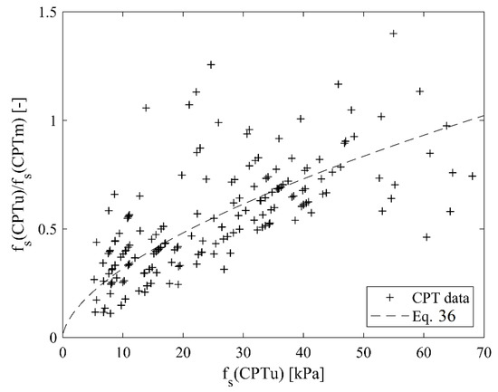
Figure 5.
Correlation function between fs(CPTm) and fs(CPTu).
The correlation is applicable only when fs < 65 kPa. Thus, fs(CPTm) can be corrected according to Equations (36) and (37) in order to obtain a reasonable estimate of the corresponding value of fs(CPTu).
4.3.2. Soil Classification Index IC Correction
The use of soil behavior type classification charts (i.e., SBT and SBTn charts by Robertson [38,39] and Robertson and Wride [16]), which are based on CPTu, for the interpretation of CPTm generally results in an underestimation of the soil grain size. To enable the use of SBTn classification also in the case of CPTm, a correction factor, ΔIC, as a function of the cone tip resistance (qc) was suggested by Meisina et al. [41]. ΔIC was defined by establishing a correspondence between the soil classes of the Schmertmann chart [56] and the SBTn classes [16,38,39] (Table 5). For this purpose, a database of 78 CPTm was used. Tests had been carried out in Mirabello, San Carlo, and Sant’Agostino (municipalities located in Emilia-Romagna region and hit by the 2012 Emilia-Romagna seismic sequence). Test results were interpreted using both the Schmertmann [56] and SBTn classification systems. A total of 6141 CPTm measurements were used and the correspondence between these two classification systems, as shown in Table 5, was checked. A perfect match between these systems was achieved in 35% of the cases, and was mainly observed for SBTn classes 3, 4, and 5. The SBTn system underestimated of one and two classes the Schmertmann [56] classification in 24% and 16% of the cases, respectively, while it overestimated of one and two classes the Schmertmann classification in 20% and 5% of the cases, respectively. The SBTn overestimate (OE) mainly concerned clayey soils and the SBTn underestimate (UE) was especially observed in sandy soils.
Table 5.
Correspondence between Schmertmann [56] and Robertson [38] classification systems (classes 1 and 9 of the Robertson approach were not considered).
Figure 6 clearly shows that the SBTn class 6 has a limited number of cases, while classes 7 and/or 8 are completely absent. On the contrary, the Schmertmann chart [56] exhibits a relevant number of points in the sand and silt/sand areas (Figure 7).
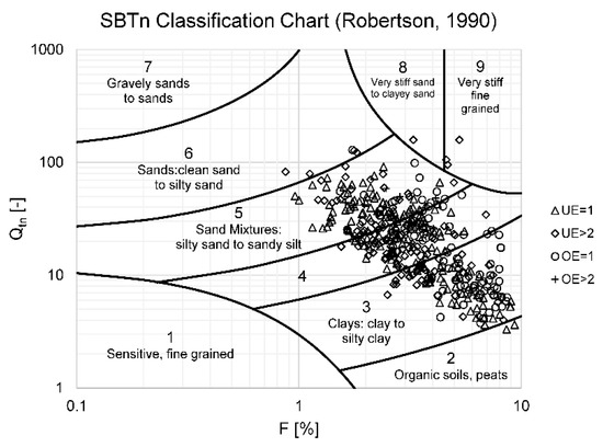
Figure 6.
Soil classification from the CPTm results according to Robertson [38].
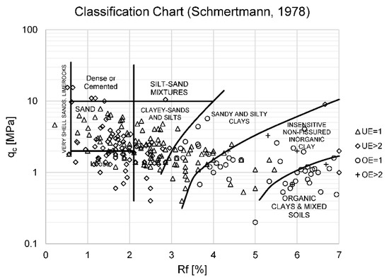
Figure 7.
Soil classification from the CPTm results according to Schmertmann [56].
The necessary correction factor, ΔIC, to have a correct match between the two classification systems (Table 5) was thus defined. The proposed correction applies only when the Robertson [38] classification underestimates that of Schmertmann [56] (Equation (38)):
where IC(OV) is the computed Ic index (Equation (13)) according to the SBTn system (Robertson, [38]; Robertson and Wride [16]) and IC(PM) is the central value of IC (Table 5) corresponding to the SBTn class that matches the Schmertmann [56] classification (clayey soils were not considered). Figure 8 shows the correction factor ΔIC as a function of qc.
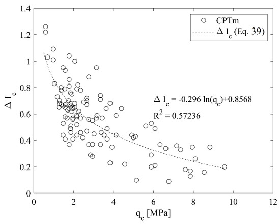
Figure 8.
Variation of ΔIc vs. qc.
The relationship between the correction factor ΔIC and the qc inferred by cone testing with a mechanical tip (CPTm) is defined by Equation (39) and should be applied to the IC index (Equation (13)), obtained according to Robertson [38] and Robertson and Wride [16], as shown in Equation (40):
The correlations presented in Equations (36) and (39) were applied to several pairs of adjacent CPTm and CPTu tests available in the database of the Emilia-Romagna region [41,42]. SBTn profiles inferred by CPTm and CPTu tests were also compared with available borehole profiles. It was confirmed that the use of classification methods that were developed to interpret CPTu mainly causes the loss of sandy to silty liquefiable layers if applied to measured CPTm data [43,57]. Thus, the application of these correlations was shown to be useful to improve the capabilities in identifying the soil layering and liquefiable layers by CPTm. The effectiveness of the correlations was also demonstrated in terms of liquefaction severity indexes [41,42]. In fact, after the application of the correction procedure, the LPI profiles from CPTm were very similar to those obtained from CPTu. Both sites in which liquefaction occurred and sites in which liquefaction did not occur were considered. The predicted liquefaction hazard was consistent with liquefaction phenomena that were observed during the 2012 seismic sequence of Emilia-Romagna.
5. Liquefaction Hazard Assessment: CPTu vs. CPTm
The correctness of the proposed approach was verified by considering both some sites in the study area as well other sites in the Emilia-Romagna region (the method was developed by considering 78 pairs of CPTu and CPTm). Table 6 summarizes the relevant information for all the pairs of CPTu and CPTm considered. In Table 6, the first two columns represent the identification code of the CPT tests considered as reported in the Tuscany and Emilia-Romagna databases. Table 6 reports the distances between each CPTm and the respective CPTu test. The pairs of CPTm and CPTu tests in the Tuscany region were available for the following three municipalities: Camaiore (sandy site), Pontedera (clayey site), and Vicchio (sandy site).
Table 6.
Pairs of CPTm and CPTu in the study area (Tuscany region) and in Emilia-Romagna.
Figure 9 compares the outcome, in terms of LPI, of the application of the three LEPs [16,19,24] for the 14 CPTu tests in Table 6. As can be observed, these three LEPs provide very similar results. Indeed, these LEPs were developed based on CPTu tests. Nearly zero values of the LPI were obtained from the CPTs in the municipality of Pontedera, which is characterized by clayey deposits.
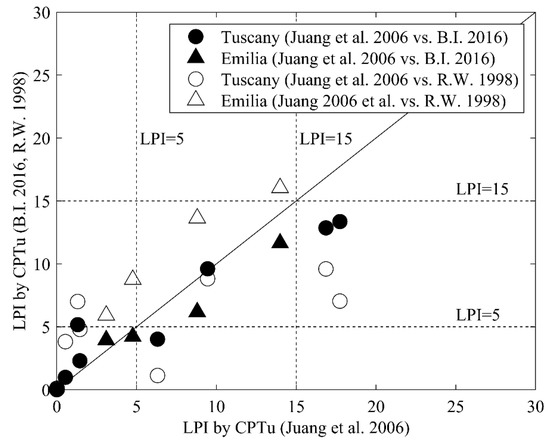
Figure 9.
Comparison between the values of the Liquefaction Potential Index (LPI) obtained with CPTu by using all the considered liquefaction evaluation procedures (LEPs). B.I. = Boulanger and Idriss; R.W. = Robertson and Wride.
In contrast, Figure 10 and Figure 11 show the LPI values obtained by using the considered LEPs in the 14 CPTm tests in Table 6 without (w/o) and with applying the correction procedure described in Section 4.3, respectively. Figure 10 clearly shows that the application of these LEPs to uncorrected CPTm data results in an underestimation of the LPI values in all the 14 cases if compared to those in Figure 9, and that the LEPs are no longer in good agreement.
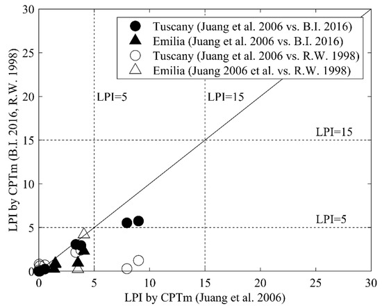
Figure 10.
Comparison between the values of the LPI obtained with uncorrected CPTm data by using all the considered LEPs. B.I. = Boulanger and Idriss; R.W. = Robertson and Wride.
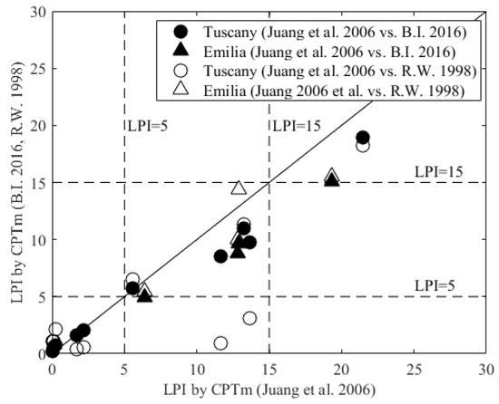
Figure 11.
Comparison between the values of the LPI obtained with corrected CPTm data by using all the considered LEPs. B.I. = Boulanger and Idriss; R.W. = Robertson and Wride.
Figure 11 shows that the application of the correction procedure, which involves some corrections to the measured fs and estimated IC, permits to obtain LPI values which are closer to or higher than those obtained from CPTu tests (Figure 9). This is clearly shown in Figure 12 in which the LPI by CPTu and the LPI by CPTm (with and w/o corrections) are compared when considering the LEPs developed by Boulanger and Idriss [24] and Juang et al. [19]. In any case, there is no historical evidence of liquefaction phenomena in the study areas (Tuscany) to confirm the correctness of the predictive capacity of the considered LEPs.
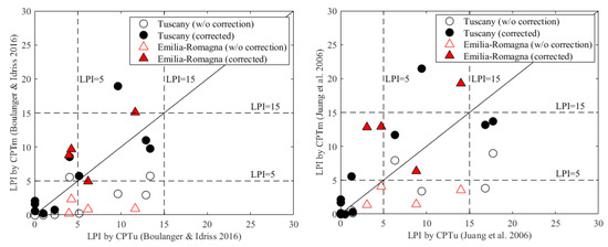
Figure 12.
Comparison between the values of the LPI obtained with CPTu and CPTm (with and w/o corrections) by using the LEPs proposed by Boulanger and Idriss [24] (left) and Juang et al. [19] (right).
The CPTm-CPTu pair (CPTu 13-CPTm 6, Table 6) in the Vicchio site is used here to demonstrate the effectiveness of the correction procedure [41,42]. Figure 13 shows measured qc, fs, and computed IC (Robertson and Wride [16]) profiles as obtained from CPTu (black continuous line) and CPTm (red dashed line). Corrected fs and Ic values are those blue points that are not located above the red dashed lines (uncorrected CPTm data). In this site, the GWT was located 2.0 m below the ground level. The correction procedure mainly modifies the fs and IC values between 1–2 and 5–8 m in depth. Therefore, the corrected values of fs and IC modify the LPI.
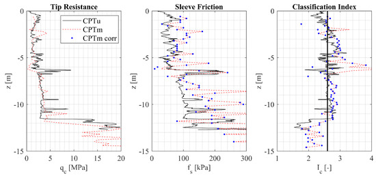
Figure 13.
qc(z), fs(z), and IC(z) profiles (CPTu 13, CPTm 6, and CPTm 6 corrected, Vicchio site).
Figure 14 shows the effect of the corrections by using the Boulanger and Idriss [24], Robertson and Wride [16], and Juang et al. [19] LEPs, respectively, in terms of LPI profiles. Looking at Figure 14, the LPI values obtained from CPTm after corrections are closer to those inferred from CPTu for the test site considered.
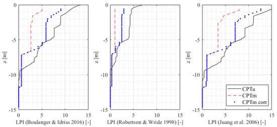
Figure 14.
LPI(z) profiles obtained by using the three LEPs considered (CPTu 13, CPTm 6, and CPTm 6 corrected).
6. Liquefaction Hazard Assessment for the Study Area
The three considered LEPs and the correction procedure were applied to the whole CPT database to assess the liquefaction hazard of the study areas. Table 7, Table 8 and Table 9 and Figure 15, Figure 16 and Figure 17 summarize the results. In Table 7 (Versilia macro-area) and 9 (Pisa plain macro-area), the results refer to those CPTm and CPTu with depths equal to or higher than 15 m. In Table 8 (Lucca plain macro-area), due to the limited number of CPTm and CPTu tests the results refer to those tests with depths equal to or higher than 10 m. As already shown, the methods give different results even without any correction in the case of CPTm. These differences are not due to the proposed correction procedure but are intrinsic differences among different LEPs. More specifically, the Juang et al. [19] and Boulanger and Idriss [24] methods give similar estimates of LPI.
Table 7.
Liquefaction severity classes for the macro-area of Versilia (CPTs with depth ≥ 15 m).
Table 8.
Liquefaction severity classes for the macro-area of the Lucca plain (CPTs with depth ≥ 10 m).
Table 9.
Liquefaction severity classes for the macro-area of the Pisa plain (CPTs with depth ≥ 15 m).
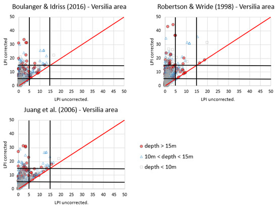
Figure 15.
LPI (corrected) vs. LPI (w/o corrections) for the macro-area of Versilia.
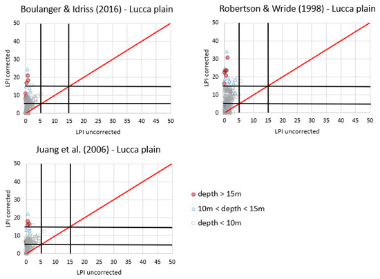
Figure 16.
LPI (corrected) vs. LPI (w/o corrections) for the macro-area of the Lucca plain.
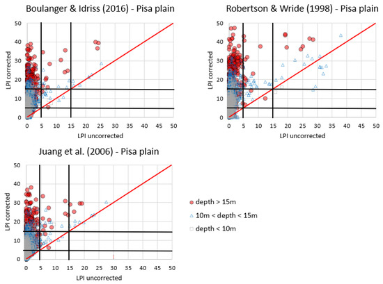
Figure 17.
LPI (corrected) vs. LPI (w/o corrections) for the macro-area of the Pisa plain.
When applying the proposed approach to the whole database, the Robertson and Wride [16] method gives the higher increase of the LPI, whereas in the case of the Boulanger and Idriss [24] and Juang et al. [19] LEPs, the increase of the LPI is less dramatic.
In more detail, it is possible to observe that:
- (1)
- for the Versilia macro-area (Table 7, Figure 15), where most of the available tests were carried out down to depths of 5–8 m (31%) and 8–10 m (24%), the three LEPs without applying the fs and Ic corrections agree to recognize a zero or low severity for most of the tests. After applying the corrections described in Section 4.3 to the Robertson and Wride [16] method, the high severity and very high severity classes increase from 11.9% and 2.0% to about 45.5% and 20.8%, respectively (considering only those tests with depths equal to or higher than 15 m). When the corrections are applied to the Boulanger and Idriss [24] and Juang et al. [19] approaches, the increase in the high and very high severity classes is less dramatic, especially for the very high severity class (LPI > 15);
- (2)
- for the macro-area of the Lucca plain (Table 8, Figure 16), where 40% and 24% of the available tests were carried out down to depths of 5–8 m and 8–10 m, respectively, the three LEPs without applying the fs and Ic corrections agree to classify all the tests in the zero or low severity classes. Very different results are obtained after applying the corrections. In fact, only 30.5% of the tests remain in the low, 42.4% fall in the high, and 23.7% in the very high severity class by using the LEP by Robertson and Wride [16] (considering only those tests with depths equal to or higher than 10 m). After applying the corrections to the Boulanger and Idriss [24] and Juang et al. [19] approaches, especially the very high severity class increases in a negligible way;
- (3)
- for the macro-area of the Pisa plain (Table 9, Figure 17), where 49%, 17%, and 6% of the available tests were carried out down to depths of 8–10 m, 10–15 m, and greater than 20 m, respectively, the three LEPs without applying the fs and Ic corrections agree to classify most of the tests in the zero or low liquefaction severity classes. After applying the corrections, the three LEPs exhibit the same trend that was observed for the other two macro-areas, even though with different percentages.
More importantly, regardless of the large numbers of tests that were analyzed, it was not possible to define areas with very high or negligible liquefaction potential. Indeed, the LPI values were casually spread all over the study area and clustering was not possible [45]. Therefore, it is only possible to recommend the most appropriate LEP to be used for the design of new construction projects or the retrofitting of existing ones.
In order to state which of the three LEPs give more realistic predictions, it is necessary to consider the historical seismicity of the study areas as well as historical evidence of liquefaction. In particular, the following facts should be considered:
- the study area could be split into two main classes: urbanized areas that have existed for many centuries and areas that were only urbanized after the Second World War. More specifically, the near-sea plains were uninhabited until the end of the Second World War. Indeed, these areas have only been urbanized since the 1960s. The database was developed mainly to help in evaluating the liquefaction risk in recently urbanized areas;
- on the other hand, there is no historical evidence of relevant liquefaction phenomena in the historically inhabited areas. Therefore, for those areas, a low to moderate liquefaction risk is expected;
- a similar or not very different picture is expected for recently urbanized areas in the case of the same geological features (Holocene, alluvial deposits mainly consisting of sand and silt mixtures);
- it has been shown that the Robertson and Wride [16] approach gives higher values of the LPI. On the other hand, the applied corrections have the only aim of obtaining the same predictions from both CPTm and CPTu. The results obtained with this approach could have been affected by the assumptions we made regarding some factors (i.e., rd, MSF and Kσ);
- therefore, the above considerations suggest that the corrected Boulanger and Idriss [24] and Juang et al. [19] approaches could be the most appropriate for the study area.
Moreover, the execution of additional “deep” CPTu tests in the study area is underway and will help in clarifying some aspects of the proposed approach that remain not well defined, even though this will take a long time for several reasons. The GIS-referenced database and the liquefaction hazard analysis results as obtained with the three uncorrected and corrected LEPs are available at the Tuscany region’s website (http://www.regione.toscana.it/speciali/rischio-sismico).
7. Conclusions
A GIS-referenced database of CPTm from the coastal area of Tuscany was implemented. Unfortunately, most of the tests did not reach depths as high as 20 m. A recently proposed correction procedure was applied to CPTm data to obtain results that were similar to those inferred from CPTu. Even though the use of CPTu remains highly recommended for liquefaction hazard analyses, this methodology is a very useful tool for those countries where huge CPTm databases are available.
From the comparison between the LPI values obtained from CPTu and CPTm, it was generally found that:
- when the corrections are applied to CPTm, the three considered LEPs predict the same severity class inferred from CPTu;
- among the three LEPs used herein, those proposed by Boulanger and Idriss [24] and Juang et al. [19] lead to very similar results;
- in any case, the Robertson and Wride [16] approach leads to a conservative estimate of LPI, whereas the Boulanger and Idriss [24] and Juang et al. [19] approaches lead to less conservative LPI estimates. Nevertheless, the estimates obtained by using the Boulanger and Idriss [24] and Juang et al. [19] methods are closer to those obtained from CPTu tests, at least for the CPTm-CPTu pairs compared herein.
The application of the corrections to the whole CPTm database revealed that if these corrections are applied together with the Robertson and Wride [16] LEP, then a significant increase in the LPI values occurs, thus highlighting a high or very high liquefaction severity in most of the considered territory. This fact appears to be in contrast with the historical evidence that has never reported relevant phenomena of liquefaction in Tuscany. The application of the corrections together with the Boulanger and Idriss [24] and Juang et al. [19] LEPs leads to a less pronounced increase in the LPI values and of the liquefaction severity class. It is therefore recommended to use these two LEPs for the CPTm interpretation in the study area.
Author Contributions
Conceptualization, methodology, data curation, supervision, and writing—original draft preparation, D.L.P.; conceptualization, methodology, writing–original draft preparation, and resources, C.M.; methodology, writing—original draft preparation, and software, S.S.; analysis of data and data curation, A.M. and M.B. All authors have read and agreed to the published version of the manuscript.
Funding
This research received no external funding.
Acknowledgments
The authors thank Pagani Geotechnical Equipment (Piacenza, Italy) for its technical support.
Conflicts of Interest
The authors declare no conflict of interest.
References
- Kramer, S. Geotechnical Earthquake Engineering; Prentice Hall: Upper Saddle River, NJ, USA, 1996. [Google Scholar]
- Caputo, R.; Papathanassiou, G. Brief communication “Ground failure and liquefaction phenomena triggered by the 20 May 2012 Emilia-Romagna (Northern Italy) earthquake: Case study of Sant’Agostino-San Carlo-Mirabello zone”. Nat. Hazards Earth Syst. Sci. 2012, 12, 3177. [Google Scholar] [CrossRef]
- Papathanassiou, G.; Caputo, R.; Rapti-Caputo, D. Liquefaction phenomena along the paleo-Reno River caused by the May 20, 2012, Emilia (northern Italy) earthquake. Ann. Geophys. 2012, 55. [Google Scholar] [CrossRef]
- Emergeo Working Group. Liquefaction phenomena associated with the Emilia earthquake sequence of May-June 2012 (Northern Italy). Nat. Hazards Earth Syst. Sci. 2013, 13, 935–947. [Google Scholar] [CrossRef]
- Lo Presti, D.C.F.; Sassu, M.; Luzi, L.; Pacor, F.; Castaldini, D.; Tosatti, G.; Meisina, C.; Zizioli, D.; Zucca, F.; Rossi, G.; et al. A report on the 2012 seismic sequence in Emilia (Northern Italy). In Proceedings of the Seventh International Conference on case Histories in Geotechnical Engineering, Chicago, IL, USA, 29 April–4 May 2013. [Google Scholar]
- Vannucchi, G.; Crespellani, T.; Facciorusso, J.; Ghinelli, A.; Madiai, C.; Puliti, A.; Renzi, S. Soil liquefaction phenomena observed in recent seismic events in Emilia-Romagna Region, Italy. Int. J. Earthq. Eng. 2012, 2, 20–29. [Google Scholar]
- Lombardi, D.; Bhattacharya, S. Liquefaction of soil in the Emilia-Romagna region after the 2012 Northern Italy earthquake sequence. Nat. Hazards 2014, 73, 1749–1770. [Google Scholar] [CrossRef]
- Papathanassiou, G.; Mantovani, A.; Tarabusi, G.; Rapti, D.; Caputo, R. Assessment of liquefaction potential for two liquefaction prone areas considering the May 20, 2012 Emilia (Italy) earthquake. Eng. Geol. 2015, 189, 1–16. [Google Scholar] [CrossRef]
- Cubrinovski, M.; Bradley, B.; Wotherspoon, L.; Green, R.; Bray, J.; Wood, C.; Taylor, M. Geotechnical aspects of the 22 February 2011 Christchurch earthquake. Bull. N. Z. Soc. Earthq. Eng. 2011, 44, 205–226. [Google Scholar] [CrossRef]
- Bray, J.D.; Zupan, J.D.; Cubrinovski, M.; Taylor, M. CPT-based liquefaction assessments in Christchurch, New Zealand. In Proceedings of the Papers of the 3rd International Symposium on Cone Penetration Testing, Las Vegas, NV, USA, 12–14 May 2014. [Google Scholar]
- Maurer, B.W.; Green, R.A.; Cubrinovski, M.; Bradley, B.A. Evaluation of the liquefaction potential index for assessing liquefaction hazard in Christchurch, New Zealand. J. Geotech. Geoenviron. Eng. 2014, 140, 04014032. [Google Scholar] [CrossRef]
- Maurer, B.W.; Green, R.A.; Cubrinovski, M.; Bradley, B.A. Assessment of CPT-based methods for liquefaction evaluation in a liquefaction potential index framework. Géotechnique 2015, 65, 328–336. [Google Scholar] [CrossRef]
- Khoshnevisan, S.; Juang, H.; Zhou, Y.G.; Gong, W. Probabilistic assessment of liquefaction-induced lateral spreads using CPT—Focusing on the 2010–2011 Canterbury earthquake sequence. Eng. Geol. 2015, 192, 113–128. [Google Scholar] [CrossRef]
- Cetin, K.O.; Seed, R.B.; Der Kiureghian, A.; Tokimatsu, K.; Harder Jr, L.F.; Kayen, R.E.; Moss, R.E. Standard penetration test-based probabilistic and deterministic assessment of seismic soil liquefaction potential. J. Geotech. Geoenviron. Eng. 2004, 130, 1314–1340. [Google Scholar] [CrossRef]
- Seed, H.B.; Idriss, I.M. Simplified Procedure for Evaluating Soil Liquefaction Potential. J. Soil Mech. Found. Div. ASCE 1971, 97, 1249–1273. [Google Scholar]
- Robertson, P.K.; Wride, C.E. Evaluating Cyclic Liquefaction Potential Using the Cone Penetration Test. Can. Geotech. J. 1998, 35, 442–459. [Google Scholar] [CrossRef]
- Youd, T.L. Liquefaction resistance of soils: Summary report from the 1996 NCEER and 1998 NCEER/NSF workshops on evaluation of liquefaction resistance of soils. J. Geotech. Geoenviron. Eng. 2001, 127, 817–833. [Google Scholar] [CrossRef]
- Juang, C.H.; Yuan, H.; Lee, D.H.; Lin, P.S. Simplified cone penetration test-based method for evaluating liquefaction resistance of soils. J. Geotech. Geoenviron. Eng. 2003, 129, 66–80. [Google Scholar] [CrossRef]
- Juang, C.H.; Fang, S.Y.; Khor, E.H. First-order reliability method for probabilistic liquefaction triggering analysis using CPT. J. Geotech. Geoenviron. Eng. 2006, 132, 337–350. [Google Scholar] [CrossRef]
- Moss, R.E.; Seed, R.B.; Kayen, R.E.; Stewart, J.P.; Der Kiureghian, A.; Cetin, K.O. CPT-based probabilistic and deterministic assessment of in situ seismic soil liquefaction potential. J. Geotech. Geoenviron. Eng. 2006, 132, 1032–1051. [Google Scholar] [CrossRef]
- Idriss, I.M.; Boulanger, R.W. Semi-empirical procedures for evaluating liquefaction potential during earthquakes. J. Soil Dyn. Earthq. Eng. 2006, 26, 115–130. [Google Scholar] [CrossRef]
- Idriss, I.M.; Boulanger, R.W. Soil Liquefaction during Earthquakes; Earthquake Engineering Research Institute: Oakland, CA, USA, 2008. [Google Scholar]
- Boulanger, R.W.; Idriss, I.M. CPT and SPT Based Liquefaction Triggering Procedures; Report No. UCD/CGM-14/01; Center for Geotechnical Modeling, Department of Civil and Environmental Engineering, University of California: Davis, CA, USA, 2014; p. 134. [Google Scholar]
- Boulanger, R.W.; Idriss, I.M. CPT-based liquefaction triggering procedure. J. Geotech. Geoenviron. Eng. 2016, 142, 04015065. [Google Scholar] [CrossRef]
- Robertson, P.K.; Campanella, R.G. Liquefaction potential of sands using the cone penetration test. J. Geotech. Div. ASCE 1985, 22, 277–286. [Google Scholar]
- Yuan, H.; Yang, S.H.; Andrus, R.D.; Juang, C.H. Liquefaction-induced ground failure: A study of the Chi-Chi earthquake cases. Eng. Geol. 2004, 71, 141–155. [Google Scholar] [CrossRef]
- Kayabali, K. Soil liquefaction evaluation using shear wave velocity. Eng. Geol. 1996, 44, 121–127. [Google Scholar] [CrossRef]
- Andrus, R.D.; Stokoe, K.H. Liquefaction Resistance of Soils from Shear-Wave Velocity. J. Geotech. Geoenviron. Eng. 2000, 126, 1015–1025. [Google Scholar] [CrossRef]
- Vaid, Y.P.; Hughes, J.M.; Byrne, P.M. Dilation Angle and Liquefaction Potential. J. Geotech. Eng. Div. 1981, 107, 1003–1008. [Google Scholar]
- Robertson, P.K.; Campanella, R.G. Estimating liquefaction potential of sands using the flat plate dilatometer. Geotech. Test. J. 1986, 9, 38–40. [Google Scholar]
- Tsai, P.H.; Lee, D.H.; Kung, G.T.C.; Juang, C.H. Simplified DMT-based methods for evaluating liquefaction resistance of soils. Eng. Geol. 2009, 103, 13–22. [Google Scholar] [CrossRef]
- Iwasaki, T.; Tokida, K.; Tatsuko, F.; Yasuda, S. A practical method for assessing soil liquefaction potential based on case studies at various sites in Japan. In Proceedings of the 2nd International Conference on Microzonation for Safer Construction-Research and Application, San Francisco, CA, USA, 26 November–1 December 1978; Volume 2, pp. 885–896. [Google Scholar]
- Tonkin and Taylor. Liquefaction Vulnerability Study; Tonkin e Taylor Ltd.: Auckland, New Zealand, 2013. [Google Scholar]
- Sonmez, H. Modification of the liquefaction potential index and liquefaction susceptibility mapping for a liquefaction-prone area (Inegol, Turkey). Environ. Geol. 2003, 44, 862–871. [Google Scholar] [CrossRef]
- Mayne, P.W. Synthesis 368: Cone Penetration Testing. NCHRP; Transportation Research Board, National Academy Press: Washington, DC, USA, 2007. [Google Scholar]
- Boulanger, R.W.; DeJong, J.T. Inverse filtering procedure to correct cone penetration data for thin-layer and transition effects. In Proceedings of the Cone Penetration Testing 2018, Delft, The Netherlands, 21–22 June 2018; pp. 25–44. [Google Scholar]
- Robertson, P.K.; Campanella, R.G.; Gillespie, D.; Greig, J. Use of piezometer cone data. In Use of in Situ Tests in Geotechnical Engineering; ASCE: Reston, VA, USA, 1986; pp. 1263–1280. [Google Scholar]
- Robertson, P.K. Soil Classification Using the Cone Penetration Test. Can. Geotech. J. 1990, 27, 151–158. [Google Scholar] [CrossRef]
- Robertson, P.K. Interpretation of cone penetration tests—A unified approach. Can. Geotech. J. 2009, 46, 1337–1355. [Google Scholar] [CrossRef]
- Lo Presti, D.; Meisina, C.; Squeglia, N. Use of cone penetration tests for soil profiling. Ital. Geotech. J. 2009, 2, 9–33. [Google Scholar]
- Meisina, C.; Persichillo, M.G.; Francesconi, M.; Creatini, M.; Lo Presti, D.C. Differences between mechanical and electrical cone penetration test in the liquefaction hazard assessment and soil profile reconstruction. In Proceedings of the ICCE International Conference of Civil Engineering, Tirana, Albania, 12–14 October 2017; pp. 95–105. [Google Scholar]
- Meisina, C.; Stacul, S.; Lo Presti, D. Empirical correlations to improve the use of mechanical CPT in the liquefaction potential evaluation and soil profile reconstruction. In Proceedings of the 4th International Symposium on Cone Penetration Testing, CPT’18, Delft, The Netherlands, 21–22 June 2018; p. 435. [Google Scholar]
- Lo Presti, D.; Giusti, I.; Cosanti, B.; Squeglia, N.; Pagani, E. Interpretation of CPTu in “unusual” soils. Riv. Ital. Geotec. 2016, 4, 25–44. [Google Scholar]
- Regione Emilia Romagna (Italy). La Banca Dati Geognostica. 2011. Available online: http://ambiente.regione.emilia-romagna.it/geologia/cartografia/webgis-banchedati/banca-dati-geognostica (accessed on 3 February 2020).
- Regione Toscana. Geoscopio: Geological Database. 2019. Available online: http://www502.regione.toscana.it/geoscopio/geologia.html (accessed on 3 February 2020).
- NTC. Norme Tecniche per le Costruzioni 2018. Aggiornamento delle ‘Norme tecniche per le costruzioni’. Gazzetta Ufficiale Serie Generale n.42 del 20-02-2018—Suppl. Ordinario n. 8. Italian Building Code (in Italian). 2018. Available online: https://www.gazzettaufficiale.it/eli/id/2018/2/20/18A00716/sg (accessed on 3 February 2020).
- Galli, P.; Meloni, F. Liquefazione Storica. Un catalogo nazionale. Quat. Ital. J. Quat. Sci. 1993, 6, 271–292. [Google Scholar]
- Groholski, D.R.; Hashash, Y.M.; Kim, B.; Musgrove, M.; Harmon, J.; Stewart, J.P. Simplified model for small-strain nonlinearity and strength in 1D seismic site response analysis. J. Geotech. Geoenviron. Eng. 2016, 142, 04016042. [Google Scholar] [CrossRef]
- Angina, A.; Steri, A.; Stacul, S.; Lo Presti, D. Free-Field Seismic Response Analysis: The Piazza dei Miracoli in Pisa Case Study. Int. J. Geotech. Earthq. Eng. 2018, 9, 1–21. [Google Scholar] [CrossRef]
- Fiorentino, G.; Nuti, C.; Squeglia, N.; Lavorato, D.; Stacul, S. One-dimensional nonlinear seismic response analysis using strength-controlled constitutive models: The case of the leaning tower of Pisa’s subsoil. Geosciences 2018, 8, 228. [Google Scholar] [CrossRef]
- Liao, S.S.C.; Whitman, R.V. Catalogue of Liquefaction and Non-Liquefaction Occurrences during Earthquakes; Res. Rep. Dept. of Civ. Engrg.; Massachusetts Institute of Technology: Cambridge, MA, USA, 1986. [Google Scholar]
- Spallarossa, D.; Barani, S. Disaggregazione della pericolosità sismica in termini di MR-ε. Progetto DPC-INGV S1 Deliv. D14 2007. [Google Scholar]
- Pagani Geotechnical Equipment. 2017. Available online: http://www.pagani-geotechnical.com (accessed on 3 February 2020).
- Viggiani, C.; Pepe, M. Il Sottosuolo della Torre. In La Torre Restituita; Gli Studi e gli Interventi che Hanno Consentito la Stabilizzazione Della Torre di Pisa; Poligrafico dello Stato: Rome, Italy, 2005. [Google Scholar]
- Squeglia, N.; Stacul, S.; Abed, A.A.; Benz, T.; Leoni, M. m-PISE: A novel numerical procedure for pile installation and soil extraction. Application to the case of Leaning Tower of Pisa. Comput. Geotech. 2018, 102, 206–215. [Google Scholar] [CrossRef]
- Schmertmann, J.H. Guidelines for Cone Penetration Test. In Performance and Design; U.S. Department of Transportation: Washington, DC, USA, 1978. [Google Scholar]
- Lo Presti, D.; Stacul, S.; Meisina, C.; Bordoni, M.; Bittelli, M. Preliminary Validation of a Novel Method for the Assessment of Effective Stress State in Partially Saturated Soils by Cone Penetration Tests. Geosciences 2018, 8, 30. [Google Scholar] [CrossRef]


© 2020 by the authors. Licensee MDPI, Basel, Switzerland. This article is an open access article distributed under the terms and conditions of the Creative Commons Attribution (CC BY) license (http://creativecommons.org/licenses/by/4.0/).