Abstract
This paper presents the results from a study on the application of an artificial neural network (ANN) model for regional flood frequency analysis (RFFA). The study was conducted using stream flow data from 88 gauging stations across New South Wales (NSW) in Australia. Five different models consisting of three to eight predictor variables (i.e., annual rainfall, drainage area, fraction forested area, potential evapotranspiration, rainfall intensity, river slope, shape factor and stream density) were tested. The results show that an ANN model with a higher number of predictor variables does not always improve the performance of RFFA models. For example, the model with three predictor variables performs considerably better than the models using a higher number of predictor variables, except for the one which contains all the eight predictor variables. The model with three predictor variables exhibits smaller median relative error values for 2- and 20-year return periods compared to the model containing eight predictor variables. However, for 5-, 10-, 50- and 100-year return periods, the model with eight predictor variables shows smaller median relative error values. The proposed ANN modelling framework can be adapted to other regions in Australia and abroad.
1. Introduction
Globally, floods are the most damaging natural disasters that cause enormous economic loss and social disruptions across the landscape. In the last decade, floods accounted for roughly 45% of all disasters (and people affected by them) and caused an average of 6000 casualties in each year [1]. Floods cause billions of dollars of damage annually worldwide, and even in the world’s driest inhabited continent, Australia, flooding is the costliest natural disaster [1,2,3]. In recent years, floods have become more frequent and highly disastrous due to global climate change [1].
One of the key steps in flood risk assessment process is the estimation of design floods [2]. A design flood is the peak discharge used to design hydraulic structures (e.g., bridge, culvert, retaining wall) and the magnitude of the flood is represented by the annual exceedance probability (AEP) [4]. At-site flood frequency analysis is the commonly accepted method to estimate design flood in a gauged catchment if observed streamflow data are available for a number of years. However, there are numerous catchments where observed streamflow data are not available. Regional flood frequency analysis (RFFA) is considered as the best option to estimate design flood for these catchments [5,6,7].
The efficiency of a RFFA technique primarily depends on two factors: (i) sufficiency and accuracy of historical streamflow data in terms of record length and spatial coverage over the study area; and (ii) the adopted regionalization method that explores flood characteristics in gauged catchments and transfers the relevant flood attributes to ungauged catchments. Some of the most successful RFFA techniques include (i) an index flood estimation method [8], (ii) a quantile regression method [9] and (iii) a parameter regression method [10,11]. All of these techniques are essentially linear, such that floods are linearly related with catchment characteristics either in a log domain or domain with raw data [12,13].
While efforts have been made to develop nonlinear RFFA methods to estimate design floods, the application of such methods are quite limited. In the past few years, some non-linear methods, such as an artificial neural network (ANN), gene expression programming and fuzzy models, were developed and their efficiency was evaluated [12,13]. Aziz et al. [13] investigated the performances of ANN and GEP methods using streamflow records from 452 gauging stations across Australia. They compared the results with quantile regression technique, which is a linear RFFA method, and concluded that a non-linear method produced better results compared to a linear method.
The working principle of ANN is similar to that of the human neural system [14]. Unlike other data processing methods which learn through programming, an ANN model investigates the patterns in a data set and correlate them. The ANN consists of simple computing units called ‘artificial neurons’. Each unit is connected to the other units via weight connectors. These units calculate the sum of all weighted inputs and bias. It then produces output of previously weighted input and bias using an activation function.
In the last few decades, the ANN model (introduced by McCulloch and Pitts [15]) has been extensively used to solve various mathematical problems, especially in the field of medical science [14,16,17]. In recent years, the method has been used in engineering fields for forecasting and data compression. Lapedes and Farber [18] applied the ANN model to investigate non-linear data series and found better generalization capabilities of ANN models compared to a regression-based model. ANN model is more capable of identifying non-linear connections between observed and predicted data sets [19,20].
In the Australian context, studies on ANN-based RFFA modelling are limited. The majority of previous RFFA studies have been based on linear models [5,10]. Aziz et al. [21,22] applied ANN-based RFFA modelling; however, they applied a limited set of catchment characteristics in model building. The objectives of this study are: (i) to develop and test ANN-based RFFA models using a higher number of catchment attributes; and (ii) to recommend the best ANN-based RFFA model containing an optimum number of predictor variables for the catchments in New South Wales.
2. Principle of ANN
The concept of an ANN model is schematically represented in Figure 1. The first column represents various input variables () and the second column represents the specific weight of input variables (). The output is determined by considering a given vector. There is a constant value (1) among the inputs which has been introduced to the neuron by its unique weight, known as bias (b). Bias allows the ANN to change the activation function. It is important to note that bias is not essential for a network but it helps in improving the performance of a network significantly [23].
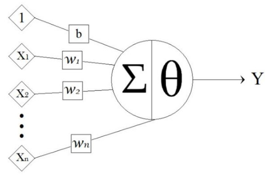
Figure 1.
Conceptual representation of an artificial neural network (ANN) model.
Mathematically, the input (I) and output (Y) of a neuron in an ANN model can be represented as [23]:
where X is the input, W is the weight, b is the bias and θ is the sum of all weighted inputs.
The output of a neuron can be presented by different activation functions. A sigmoid function (Equation (2)) is a commonly used activation function for such outputs [24]. This sigmoid function maps the data between 1 and 0 (Figure 2). A sigmoid function is adopted in this study because it is a bounded differentiable function. It is defined for all real inputs and at each point it produces a non-negative derivative [21,22]. Other activation functions could have been adopted; however, the use of the sigmoid function is deemed adequate in this study. The dependent and predictor variables in this study are normalized to achieve zero mean and unit variance for each of the variables.
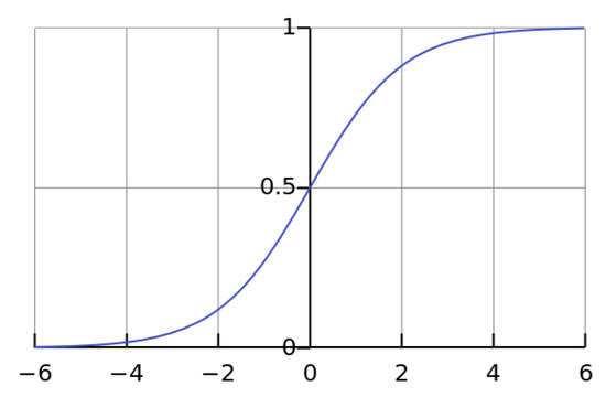
Figure 2.
Representation of a sigmoid function.
Figure 3 shows a configuration of an ANN model with interlinking between the input and output data layers. It consists of three input neurons, two hidden layers of three and two percepterons and an output layer with two output neurons.
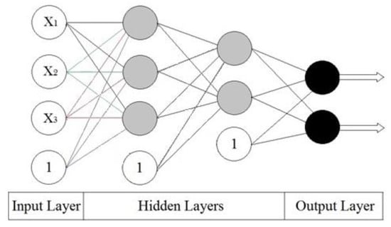
Figure 3.
Schematic diagram of an ANN model with two hidden layers.
In recent years, the application of ANN model has increased in rainfall-runoff modelling, groundwater modelling, streamflow forecasting and water quality modelling (e.g., [25,26,27,28,29,30]). Table 1 presents a list of relevant literature which used ANN successfully in solving hydrological and related problems. It can be seen that the majority of studies used the feed forward (FF) algorithm in the ANN architecture, back propagation (BP) for optimization, and log normal as a transfer function (Table 1). In FF neural networks, the information only travels forward in the neural network through the input nodes, then through the hidden layers and finally through the output nodes [23]. Optimization is used for the fine-tuning of weights factors in ANN modelling based on the errors in the previous iteration [23].

Table 1.
List of studies on ANN in the field of hydrological modelling (1992–2019).
3. Materials and Methods
Data from 88 stream gauging stations across New South Wales (NSW) were used to develop the ANN model (Figure 4). Selected gauges were situated on natural streams and free from any major regulation. Drainage area between the selected gauging stations varied from 8 to 1010 km2. The first, second (median) and third quartile drainage area were 142.5, 260 and 537.25 km2, respectively. The streamflow data of the selected stream gauging stations were downloaded from the WaterNSW website [85]. The periods of annual maximum (AM) flow records at these stream gauging stations varied between 25 to 82 years. This study was conducted based on eight predictor variables that included (i) mean annual rainfall (MAR); (ii) areal potential evapo-transpiration (MAE), (iii) drainage area (AREA) (iv) 6-hour duration rainfall for a 2-year return period (I62); (v) shape factor (SF); (vi) stream density (SDEN); (vii) river slope (S1085) and (viii) proportion of forest (FOREST).
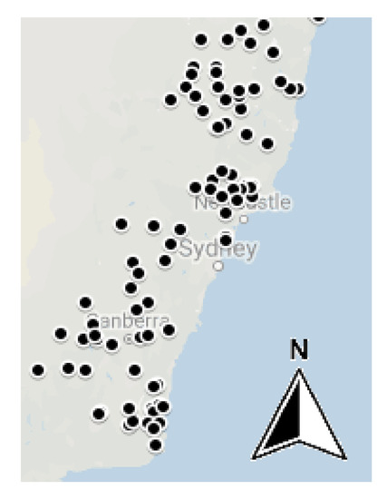
Figure 4.
Location of selected stream gauging stations in New South Wales, Australia.
A 1:100,000 topographic map was used to delineate catchment boundary and drainage area for individual gauge. Rainfall intensity data (I62) were obtained from the online portal of Australian Bureau of Meteorology (BOM) using intensity-frequency-duration (IFD) estimation tool [86]. The MAR and MAE data at the catchment centroid were extracted from Australian Bureau of Meteorology website [86]. The shape factor (SF) for a catchment was considered as the shortest distance between catchment outlet and centroid divided by the square root of the drainage area. The SDEN was calculated as a ratio of the stream length (total length for all streams in a catchment) and drainage area. Stream length was measured on a 1:100,000 topographic map using a digital distance meter. The forested area for a catchment was measured on 1:100,000 topographic map using a planimeter. The minimum, maximum and median parameter values are presented in Table 2.
Table 2.
Summary of catchment data used in this study.
Five different ANN-based RFFA models were selected to assess their performances (Table 3). Model 1 consisted of all the eight predictor variables. Other models consisted of more than one but less than eight variables. It is important to note that models were selected based on the best potential combination, but there could be other combinations as well. As recommendations in previous RFFA studies, rainfall intensity was included in all five models and drainage area was selected as the predictor variable [70,87].
Table 3.
Five different ANN based regional flood frequency analysis (RFFA) models with adopted catchment characteristics represented by green colour (predictor variables).
Six flood events of discharge magnitudes 2 (Q2), 5 (Q5), 10 (Q10), 20 (Q20), 50 (Q50) and 100 (Q100) years return period were used as dependent variables. Design flood discharges were estimated by fitting the Log Pearson type III (LP3) probability distribution function to the observed annual maximum flood discharge [88,89]. The analyses were conducted using the FLIKE software, which is commonly used for flood frequency modelling in Australia [90]. The main advantage of FLIKE is that it fits five probability distribution functions for a given set of flood data and identifies the best frequency model for that data set [91]. In this study, LP3 was selected because it was found as the best fit distribution for Australian stream gauge data [10].
A 2-layer feed forward neural network and with a backpropagation algorithm was selected in this study.
The selected 88 stream gauging stations were sub-divided into three sets. Group 1 consisted of 62 stations (70%) and they were used for model training, Group 2 consisted of 13 stations (15%) and they were used for validation. The third group (13 stations), were used to evaluate model performances in predictions. It is important to note that the gauges in each group were selected randomly. The analyses were conducted using a two-layer FF neural network with two hidden layers in each model setup. The Levenberg–Marquardt algorithm was used for model training. The activation function was represented in the model using a hyperbolic sigmoid function. The entire analyses were carried out using MATLAB software. A set of statistical tests were performed to evaluate the model performance. These include, root mean squared error (RMSE), root mean squared normalised error (RMSNE), relative root mean squared error (RRMSE), coefficient of determination (R2), mean bias (BIAS), relative mean bias in percent (rBIAS), absolute relative error (abs-RE) and quantile ratio (r, ratio of predicted and observed discharge) as presented in Equations (3–10). These evaluation statistics were adopted from Bloschl et al. [92].
where and are the predicted and observed flood discharge, respectively, is the mean observed discharge and n is the number of stations.
4. Results and Discussion
Models performances in predicting flood quantiles are presented in Table 4 in terms of abs-RE and R2. The results show that all the models perform well for the majority of quantiles, except for Q2 by Model 1 (61%), Q5 by Model 4 (80%) and Q2 (320%) and Q5 (85%) by Model 5. Model 2 (two predictor variables) performed reasonably well with the lowest and highest RE of 32.9% and 47.7%, respectively. For all five quantiles, Model 3 performed very well (RE values in the range of 29.48%–52.24%). Model 4 performed well for most quantiles, except Q5. Model 5 predictions are relatively poor for all quantiles, with the worst prediction for Q2 (RE of 319.61%). Overall, Model 5 produced the poorest results among the five models.
Table 4.
Model performance in terms of absolute relative error (abs-RE) and the coefficient of determination (R2) in predicting flood quantile.
Coefficient of determination (R2) values for Q5, Q10, Q20, and Q50 show a moderate model accuracy for the Model 1 (R2 values ranging from 0.71 to 0.76). Model 2 performed well except for the Q100 (R2 value of 0.16). Model 3 performed well for Q2, Q5, Q10 and Q20. Overall, Model 1 and 3 produced better results compared to other models. Model 4 performed the best for Q2 (R2 = 0.74) and worst for Q20. As expected, R2 values for smaller ARIs (average recurrence interval) are higher than those of the large ARIs. Model 5 performed the worst for R2 value which is consistent with RE value.
Model performances in terms of RMSNE and RRMSE are presented Table 5 for all five models. In regard to RMSNE, models performed well for most quantities, except Q2 in the case of Model 1, Q20 for Model 4 and Q2, Q5 and Q100 for Model 5. The RRMSE value for Model 1 is highest for Q2, which indicates low accuracy of the prediction. Model 2 predictions are relatively better with RMSNE values of between 0.89 (Q2) and 2.47 (Q100). In addition, the best value of RRMSE is found for Q5 (0.48) and the poorest value is found for Q100 (0.85). Model 3 performed well for Q10 with the value of 0.75; however, for Q100, the RMSNE is poor with the value of 3.5. The RRMSE values for Q2, Q10 and Q20 are approximately the same (0.48). Furthermore, the values of RRMSE are the same (0.69) for Q50 and Q100. The highest error is associated with Q5, with a value of 0.82. Model 4 performed well for Q2 and Q10 with the values of 0.53 and 0.56, respectively, while the best performance was for Q50. Like other indicators, Model 5 performed the worst for RMSNE and RRMSE.
Table 5.
Model performance in terms of root mean squared normalised error (RMSNE) and relative root mean squared error (RRMSE) in predicting flood quantiles.
Table 6 presents the comparison between five models in terms of model predictions for different floods. There is no clear trend of underprediction or overprediction, nor any trend for small or large floods. All models overpredicted for some floods and underpredicted for some other floods. Overall, Model 3 produced the best result (relative bias of 33%) and Model 4 produced the worst result (relative bias of 1258%).
Table 6.
Model performance in terms of mean bias (BIAS) and relative mean bias (rBIAS) in predicting flood quantile.
Figure 5 shows a graphical comparison of model performance for predicting flood discharge for the flood events of different magnitudes. In general, Model 2 and 4 overpredicted, while other models underpredicted flood magnitude. Overall, Model 2 predictions are close to 1, which indicates a better performance. Model 5 performed the worst with predicted discharge for Q2, which is more than double the observed value.
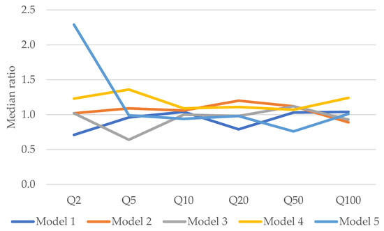
Figure 5.
Comparison of observed and predicted quantile ratio for the five models.
Figure 6 shows a comparison between five models in predicting flood quantiles. The results show similar performances by Model 1 and Model 3, with little differences in the RMSE values for all six flood quantiles. Model 5 performs relatively poorly for Q2, Q10, Q20 and Q100 and Model 4 performs poor for the Q5. Overall, Model 3’s performances are better and it is considered as the best model for predicting design flood for the catchments in NSW.
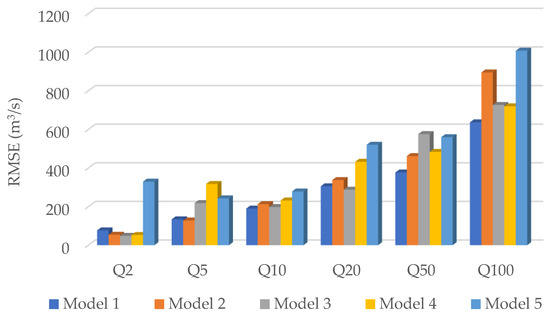
Figure 6.
Comparison of RMSE values for the five models.
The parameter setup for the Model 3 is similar to the current Australian Rainfall and Runoff (ARR) model for NSW which consists of AREA, I62 and SF as predictor variables. While Model 1 (which includes all eight predictor variables) performs well with respect to RE for all quantiles except Q2, Model 3’s performances are the best. It is important to note that none of the models are the best for all six quantiles. For example, with respect to RE, Model 3 is the best for predicting Q2 and Q20 but Model 1 is better for predicting Q5, Q10, Q50 and Q100. Model 4 performs poorly with respect to BIAS. Model 1 is the best based on R2 except for Q2 and Q100.
Table 7 compares the performance of our two best models (Model 1 and Model 3) with similar RFFA studies based on ANN. It shows that both our models provide smaller median RE than Aziz et al. [22] for higher ARIs (10–100 years). Also, in terms of R2, our models perform much better than those of Dawson et al. [58].
Table 7.
Comparison of ANN-based RFFA models reported in the literature.
The best model (Model 3) contains three predictor variables: AREA (the main scaling factor in flood generation process), I62 (the main input that triggers runoff) and SF (the factor that affects travel time of generated runoff). It has been found that the other five predictor variables (MAR, MAE, SDEN, S1085 and FOREST) have minor roles in RFFA modelling in the study area.
5. Conclusions
In this study, ANN-based regional flood frequency models are developed to estimate the design floods. The models were tested using observed discharge data from 88 catchments in NSW. Five models were tested considering two to eight predictor variables. The best combinations of predictor variables were identified based on model performance in predicting design floods of 2, 5, 10, 20, 50 and 100 years return periods. Model performances were evaluated based on nine statistical error metrics. The study found that model predictions are better when all eight predictor variables are included. However, the results based on three predictor variables were found to be close to the results for eight predictor variables. The study concludes that a high number of predictor variables does not always improve the model predictions. The use of MAR, MAE, SDEN, S1085 and FOREST as predictor variables provide little contribution in predicting design flood for an ungauged catchment. The key predictor variables are catchment area, rainfall intensity and slope factor. The findings are very useful because these predictor variables are readily available for the majority of the catchments. The results demonstrate the potential use of the ANN-based regional flood frequency model. However, further testing with larger data sets is necessary before it can be applied elsewhere.
Author Contributions
Conceptualization, S.K. and A.R.; methodology, S.K. and A.R.; software, S.K., F.K. and A.R.; validation, S.K., F.K. and A.R.; formal analysis, S.K., and M.A.A.; investigation, S.K., M.A.A., F.K. and A.R.; resources, S.K. and A.R.; writing—original draft preparation, S.K. and A.R.; writing—review and editing, M.A.A. and F.K. All authors have read and agreed to the published version of the manuscript.
Funding
This research received no external funding.
Conflicts of Interest
The authors declare that there is no conflict of interest.
References
- FitzGerald, G.; Du, W.; Jamal, A.; Clark, M.; Hou, X.Y. Flood fatalities in contemporary Australia (1997–2008). Emerg. Med. Australas. 2010, 22, 180–186. [Google Scholar] [CrossRef] [PubMed]
- Loveridge, M.; Rahman, A. Monte Carlo simulation for design flood estimation: A review of Australian practice. Australas. J. Water Resour. 2018, 22, 52–70. [Google Scholar] [CrossRef]
- Wang, Z.; Chengguang, L.; Chen, X.; Yang, B.; Zhao, S.; Bai, X. Flood hazard risk assessment model based on random forest. J. Hydrol. 2015, 527, 1130–1141. [Google Scholar] [CrossRef]
- Myronidis, D.; Ioannou, K. Forecasting the Urban Expansion Effects on the Design Storm Hydrograph and Sediment Yield using Artificial Neural Networks. Water 2018, 11, 31. [Google Scholar] [CrossRef]
- Ouarda, T.B.; Girard, C.; Cavadias, G.S.; Bobée, B. Regional flood frequency estimation with canonical correlation analysis. J. Hydrol. 2001, 254, 157–173. [Google Scholar] [CrossRef]
- Ribatet, M.; Sauquet, E.; Gresillon, J.-M.; Ouarda, T.B.M.J. A regional Bayesian POT model for flood frequency analysis. Stoch. Environ. Res. Risk Assess. 2006, 21, 327–339. [Google Scholar] [CrossRef]
- Smith, J.; Eli, R.N. Neural-Network Models of Rainfall-Runoff Process. J. Water Resour. Plan. Manag. 1995, 121, 499–508. [Google Scholar] [CrossRef]
- Thorvat, A.R.; Mujumdar, M.M. Design flood estimation for Upper Krishna Basin through RFFA. Int. J. Eng. Sci. Technol. 2011, 3, 5252. [Google Scholar]
- Ouali, D.; Chebana, F.; Ouarda, T.B.M.J. Quantile Regression in Regional Frequency Analysis: A Better Exploitation of the Available Information. J. Hydrometeorol. 2016, 17, 1869–1883. [Google Scholar] [CrossRef]
- Haddad, K.; Rahman, A. Regional flood frequency analysis in eastern Australia: Bayesian GLS regression-based methods within fixed region and ROI framework – Quantile Regression vs. Parameter Regression Technique. J. Hydrol. 2012, 430, 142–161. [Google Scholar] [CrossRef]
- Ahn, K.-H.; Palmer, R.N. Regional flood frequency analysis using spatial proximity and basin characteristics: Quantile regression vs. parameter regression technique. J. Hydrol. 2016, 540, 515–526. [Google Scholar] [CrossRef]
- Srinivas, V.V.; Tripathi, S.; Rao, A.; Govindaraju, R. Regional flood frequency analysis by combining self-organizing feature map and fuzzy clustering. J. Hydrol. 2008, 348, 148–166. [Google Scholar] [CrossRef]
- Aziz, K.; Rahman, A.; Shamseldin, A.; Shoaib, M. Regional flood estimation in Australia: Application of gene expression programming and artificial neural network techniques. In Proceedings of the 20th International Congress on Modelling and Simulation, Adelaide, Australia, 1–6 December 2013. [Google Scholar]
- Agatonovic-Kustrin, S.; Beresford, R. Basic concepts of artificial neural network (ANN) modeling and its application in pharmaceutical research. J. Pharm. Biomed. Anal. 2000, 22, 717–727. [Google Scholar] [CrossRef]
- McCulloch, W.S.; Pitts, W. A logical calculus of the ideas immanent in nervous activity. Bull. Math. Boil. 1943, 5, 115–133. [Google Scholar] [CrossRef]
- Baxt, W.G. Use of an Artificial Neural Network for Data Analysis in Clinical Decision-Making: The Diagnosis of Acute Coronary Occlusion. Neural Comput. 1990, 2, 480–489. [Google Scholar] [CrossRef]
- Amato, F.; López, A.; Peña-Méndez, E.M.; Vanhara, P.; Hampl, A.; Havel, J. Artificial neural networks in medical diagnosis. J. Appl. Biomed. 2013, 11, 47–58. [Google Scholar] [CrossRef]
- Lapedes, A.; Farber, R. Nonlinear signal processing using neural networks: Prediction and system modelling. In Proceedings of the IEEE international conference on neural networks, San Diego, CA, USA, 21 June 1987; p. 52. [Google Scholar]
- Hsu, K.-L.; Gupta, H.; Sorooshian, S. Artificial Neural Network Modeling of the Rainfall-Runoff Process. Water Resour. Res. 1995, 31, 2517–2530. [Google Scholar] [CrossRef]
- El-Shafie, A.; Mukhlisin, M.; Najah, A.A.; Taha, M.R. Performance of artificial neural network and regression techniques for rainfall-runoff prediction. Int. J. Phys. Sci. 2011, 6, 1997–2003. [Google Scholar]
- Aziz, K.; Rahman, A.; Fang, G.; Shrestha, S. Comparison of artificial neural networks and adaptive neuro-fuzzy inference system for regional flood estimation in Australia. In Hydrology and Water Resources Symposium 2012; Engineers Australia: Sydney, Australia, 2012; pp. 954–961. [Google Scholar]
- Aziz, K.; Rahman, A.; Fang, G.; Shrestha, S. Application of artificial neural networks in regional flood frequency analysis: A case study for Australia. Stoch. Environ. Res. Risk Assess. 2013, 28, 541–554. [Google Scholar] [CrossRef]
- Araghinejad, S. Data-Driven Modeling: Using MATLAB® in Water Resources and Environmental Engineering; Springer Science and Business Media LLC: Berlin/Heidelberg, Germany, 2014; Volume 67. [Google Scholar]
- Ito, Y. Representation of functions by superpositions of a step or sigmoid function and their applications to neural network theory. Neural Networks 1991, 4, 385–394. [Google Scholar] [CrossRef]
- Maier, H.R.; Dandy, G. The Use of Artificial Neural Networks for the Prediction of Water Quality Parameters. Water Resour. Res. 1996, 32, 1013–1022. [Google Scholar] [CrossRef]
- Wu, C.; Chau, K.-W. Rainfall–runoff modeling using artificial neural network coupled with singular spectrum analysis. J. Hydrol. 2011, 399, 394–409. [Google Scholar] [CrossRef]
- Taormina, R.; Chau, K.-W.; Sethi, R. Artificial neural network simulation of hourly groundwater levels in a coastal aquifer system of the Venice lagoon. Eng. Appl. Artif. Intell. 2012, 25, 1670–1676. [Google Scholar] [CrossRef]
- Zemzami, M.; Benaabidate, L. Improvement of artificial neural networks to predict daily streamflow in a semi arid area. Hydrol. Sci. J. 2016, 61, 1–12. [Google Scholar] [CrossRef]
- Ioannou, K.; Myronidis, D.; Lefakis, P.; Stathis, D. The use of artificial neural networks (ANNs) for the forecast of precipitation levels of lake Doirani (N. Greece). Fresenius Environ. Bull. 2010, 19, 1921–1927. [Google Scholar]
- Myronidis, D.; Ioannou, K.; Fotakis, D.; Dörflinger, G. Streamflow and Hydrological Drought Trend Analysis and Forecasting in Cyprus. Water Resour. Manag. 2018, 32, 1759–1776. [Google Scholar] [CrossRef]
- French, M.N.; Krajewski, W.F.; Cuykendall, R.R. Rainfall forecasting in space and time using a neural network. J. Hydrol. 1992, 137, 1–31. [Google Scholar] [CrossRef]
- Crespo, J.; Mora, E. Drought estimation with neural networks. Adv. Eng. Softw. 1993, 18, 167–170. [Google Scholar] [CrossRef]
- Allen, G.; le Marshall, J. An evaluation of neural networks and discriminant analysis methods for application in operational rain forecasting. Aust. Meteorol. Mag. 1994, 43, 17–28. [Google Scholar]
- Karunanithi, N.; Grenney, W.J.; Whitley, D.; Bovee, K. Neural Networks for River Flow Prediction. J. Comput. Civ. Eng. 1994, 8, 201–220. [Google Scholar] [CrossRef]
- Raman, H.; Sunilkumar, N. Multivariate modelling of water resources time series using artificial neural networks. Hydrol. Sci. J. 1995, 40, 145–163. [Google Scholar] [CrossRef]
- Clair, T.A.; Ehrman, J.M. Variations in discharge and dissolved organic carbon and nitrogen export from terrestrial basins with changes in climate: A neural network approach. Limnol. Oceanogr. 1996, 41, 921–927. [Google Scholar] [CrossRef]
- Minns, A.W.; Hall, M.J. Artificial neural networks as rainfall-runoff models. Hydrol. Sci. J. 1996, 41, 399–417. [Google Scholar] [CrossRef]
- Poff, N.L.; Tokar, S.; Johnson, P. Stream hydrological and ecological responses to climate change assessed with an artificial neural network. Limnol. Oceanogr. 1996, 41, 857–863. [Google Scholar] [CrossRef]
- Chow, T.W.S.; Cho, S.Y. Development of a recurrent Sigma-Pi neural network rainfall forecasting system in Hong Kong. Neural Comput. Appl. 1997, 5, 66–75. [Google Scholar] [CrossRef]
- Hsu, K.-L.; Gupta, H.V.; Gao, X.; Sorooshian, S.; Imam, B. Self-organizing linear output map (SOLO): An artificial neural network suitable for hydrologic modeling and analysis. Water Resour. Res. 2002, 38, 38-1–38-17. [Google Scholar] [CrossRef]
- Loke, E.; Warnaars, E.; Jacobsen, P.; Nelen, F.; do Ceu Almeida, M. Artificial neural networks as a tool in urban storm drainage. Water Sci. Technol. 1997, 36, 101–109. [Google Scholar] [CrossRef]
- Shamseldin, A.Y. Application of a neural network technique to rainfall-runoff modelling. J. Hydrol. 1997, 199, 272–294. [Google Scholar] [CrossRef]
- Tawfik, M.; Ibrahim, A.; Fahmy, H. Hysteresis Sensitive Neural Network for Modeling Rating Curves. J. Comput. Civ. Eng. 1997, 11, 206–211. [Google Scholar] [CrossRef]
- Venkatesan, C.; Raskar, S.D.; Tambe, S.S.; Kulkarni, B.D.; Keshavamurty, R.N. Prediction of all India summer monsoon rainfall using error-back-propagation neural networks. Theor. Appl. Clim. 1997, 62, 225–240. [Google Scholar] [CrossRef]
- Xiao, R.; Chandrasekar, V. Development of a neural network based algorithm for rainfall estimation from radar observations. IEEE Trans. Geosci. Remote. Sens. 1997, 35, 160–171. [Google Scholar] [CrossRef]
- Dawson, C.; Wilby, R. An artificial neural network approach to rainfall-runoff modelling. Hydrol. Sci. J. 1998, 43, 47–66. [Google Scholar] [CrossRef]
- Fernando, D.A.K.; Jayawardena, A.W. Runoff Forecasting Using RBF Networks with OLS Algorithm. J. Hydrol. Eng. 1998, 3, 203–209. [Google Scholar] [CrossRef]
- Golob, R.; Štokelj, T.; Grgič, D. Neural-network-based water inflow forecasting. Control. Eng. Pr. 1998, 6, 593–600. [Google Scholar] [CrossRef]
- Jayawardena, A.W.; Fernando, D.A.K. Use of Radial Basis Function Type Artificial Neural Networks for Runoff Simulation. Comput. Civ. Infrastruct. Eng. 1998, 13, 91–99. [Google Scholar] [CrossRef]
- Phien, H.N.; Sureerattanan, S. Neural networks for filtering and forecasting of daily and monthly streamflows. In Hydrologic Modeling, Proceedings of the International Conference On Water, Engineering, Ecology, Socio-Economics and Health Engineering, Seol National University, Seoul, Korea, 18–21 October 1999; Singh, V.P., Won Seo, I., Sonu, J.H., Eds.; Water Resources Publications: Highlands Ranch, CO, USA, 1999. [Google Scholar]
- Tokar, A.S.; Johnson, P.A. Rainfall-Runoff Modeling Using Artificial Neural Networks. J. Hydrol. Eng. 1999, 4, 232–239. [Google Scholar] [CrossRef]
- Zealand, C.M.; Burn, D.H.; Simonovic, S.P. Short term streamflow forecasting using artificial neural networks. J. Hydrol. 1999, 214, 32–48. [Google Scholar] [CrossRef]
- Luk, K.; Ball, J.; Sharma, A. A study of optimal model lag and spatial inputs to artificial neural network for rainfall forecasting. J. Hydrol. 2000, 227, 56–65. [Google Scholar] [CrossRef]
- Coulibaly, P.; Anctil, F.; Bobee, B. Daily reservoir inflow forecasting using artificial neural networks with stopped training approach. J. Hydrol. 2000, 230, 244–257. [Google Scholar] [CrossRef]
- Luk, K.C.; Ball, J.; Sharma, A. An application of artificial neural networks for rainfall forecasting. Math. Comput. Model. 2001, 33, 683–693. [Google Scholar] [CrossRef]
- Zhang, B.; Govindaraju, R. Geomorphology-based artificial neural networks (GANNs) for estimation of direct runoff over watersheds. J. Hydrol. 2003, 273, 18–34. [Google Scholar] [CrossRef]
- Rajurkar, M.; Kothyari, U.; Chaube, U. Modeling of the daily rainfall-runoff relationship with artificial neural network. J. Hydrol. 2004, 285, 96–113. [Google Scholar] [CrossRef]
- Dawson, C.; Abrahart, R.; Shamseldin, A.Y.; Wilby, R. Flood estimation at ungauged sites using artificial neural networks. J. Hydrol. 2006, 319, 391–409. [Google Scholar] [CrossRef]
- Jain, A.; Kumar, A. An evaluation of artificial neural network technique for the determination of infiltration model parameters. Appl. Soft Comput. 2006, 6, 272–282. [Google Scholar] [CrossRef]
- Riad, S.; Mania, J.; Bouchaou, L.; Najjar, Y. Rainfall-runoff model usingan artificial neural network approach. Math. Comput. Model. 2004, 40, 839–846. [Google Scholar] [CrossRef]
- Kisi, O.; Cigizoglu, H.K. Comparison of different ANN techniques in river flow prediction. Civ. Eng. Environ. Syst. 2007, 24, 211–231. [Google Scholar] [CrossRef]
- Chua, L.H.; Wong, T.S.; Sriramula, L. Comparison between kinematic wave and artificial neural network models in event-based runoff simulation for an overland plane. J. Hydrol. 2008, 357, 337–348. [Google Scholar] [CrossRef]
- Shu, C.; Ouarda, T.B.M.J. Regional flood frequency analysis at ungauged sites using the adaptive neuro-fuzzy inference system. J. Hydrol. 2008, 349, 31–43. [Google Scholar] [CrossRef]
- Sciuto, G.; Bonaccorso, B.; Cancelliere, A.; Rossi, G. Quality control of daily rainfall data with neural networks. J. Hydrol. 2009, 364, 13–22. [Google Scholar] [CrossRef]
- Toth, E. Classification of hydro-meteorological conditions and multiple artificial neural networks for streamflow forecasting. Hydrol. Earth Syst. Sci. 2009, 13, 1555–1566. [Google Scholar] [CrossRef]
- Wang, W.-C.; Chau, K.-W.; Cheng, C.-T.; Qiu, L. A comparison of performance of several artificial intelligence methods for forecasting monthly discharge time series. J. Hydrol. 2009, 374, 294–306. [Google Scholar] [CrossRef]
- Besaw, L.E.; Rizzo, D.M.; Bierman, P.; Hackett, W.R. Advances in ungauged streamflow prediction using artificial neural networks. J. Hydrol. 2010, 386, 27–37. [Google Scholar] [CrossRef]
- Shamseldin, A.Y. Artificial neural network model for river flow forecasting in a developing country. J. Hydroinformatics 2010, 12, 22–35. [Google Scholar] [CrossRef]
- Wu, C.; Chau, K.-W.; Fan, C. Prediction of rainfall time series using modular artificial neural networks coupled with data-preprocessing techniques. J. Hydrol. 2010, 389, 146–167. [Google Scholar] [CrossRef]
- Aziz, K.; Rahman, A.; Fang, G.; Shrestha, S. Application of Artificial Neural Networks for Regional Flood Estimation in Australia: Formation of Regions Based on Catchment Attributes. In Proceedings of the The Second International Conference on Soft Computing Technology in Civil, Structural and Environmental Engineering, Chania, Crete, Greece, 6–9 September 2011; Volume 97. [Google Scholar]
- Yilmaz, A.G.; Imteaz, M.; Jenkins, G. Catchment flow estimation using Artificial Neural Networks in the mountainous Euphrates Basin. J. Hydrol. 2011, 410, 134–140. [Google Scholar] [CrossRef]
- Kia, M.B.; Pirasteh, S.; Pradhan, B.; Mahmud, A.R.; Sulaiman, W.N.A.; Moradi, A. An artificial neural network model for flood simulation using GIS: Johor River Basin, Malaysia. Environ. Earth Sci. 2011, 67, 251–264. [Google Scholar] [CrossRef]
- Isik, S.; Kalin, L.; Schoonover, J.E.; Srivastava, P.; Lockaby, B.G. Modeling effects of changing land use/cover on daily streamflow: An Artificial Neural Network and curve number based hybrid approach. J. Hydrol. 2013, 485, 103–112. [Google Scholar] [CrossRef]
- Kalteh, A.M. Monthly river flow forecasting using artificial neural network and support vector regression models coupled with wavelet transform. Comput. Geosci. 2013, 54, 1–8. [Google Scholar] [CrossRef]
- Nourani, V.; Baghanam, A.H.; Adamowski, J.; Gebremichael, M. Using self-organizing maps and wavelet transforms for space–time pre-processing of satellite precipitation and runoff data in neural network based rainfall–runoff modeling. J. Hydrol. 2013, 476, 228–243. [Google Scholar] [CrossRef]
- Ramana, R.V.; Budu, K.; Kumar, S.R.; Pandey, N.G. Monthly Rainfall Prediction Using Wavelet Neural Network Analysis. Water Resour. Manag. 2013, 27, 3697–3711. [Google Scholar] [CrossRef]
- Aziz, K.; Rai, S.; Rahman, A. Application of artificial neural networks and genetic algorithm for regional flood estimation in Eastern Australia. In Hydrology and Water Resources Symposium 2014; Engineers Australia: Perth, Australia, 2014. [Google Scholar]
- Makwana, J.J.; Tiwari, M.K. Intermittent Streamflow Forecasting and Extreme Event Modelling using Wavelet based Artificial Neural Networks. Water Resour. Manag. 2014, 28, 4857–4873. [Google Scholar] [CrossRef]
- Aziz, K.; Rai, S.; Rahman, A. Design flood estimation in ungauged catchments using genetic algorithm-based artificial neural network (GAANN) technique for Australia. Nat. Hazards 2015, 77, 805–821. [Google Scholar] [CrossRef]
- Aziz, K.; Rahman, A.; Shamseldin, A.Y. Development of Artificial Intelligence Based Regional Flood Estimation Techniques for Eastern Australia. In Advanced Computational Intelligence in Healthcare-7; Springer Science and Business Media LLC: Berlin/Heidelberg, Germany, 2016; Volume 628, pp. 307–323. [Google Scholar]
- Tao, Y.; Gao, X.; Ihler, A.; Hsu, K.; Sorooshian, S. Deep neural networks for precipitation estimation from remotely sensed information. In Proceedings of the 2016 IEEE Congress on Evolutionary Computation (CEC), Vancouver, BC, Canada, 24–29 July 2016; pp. 1349–1355. [Google Scholar]
- Aziz, K.; Haque, M.M.; Rahman, A.; Shamseldin, A.Y.; Shoaib, M. Flood estimation in ungauged catchments: Application of artificial intelligence based methods for Eastern Australia. Stoch. Environ. Res. Risk Assess. 2016, 31, 1499–1514. [Google Scholar] [CrossRef]
- Lee, J.; Kim, C.; Lee, J.E.; Kim, N.W.; Kim, H. Application of Artificial Neural Networks to Rainfall Forecasting in the Geum River Basin, Korea. Water 2018, 10, 1448. [Google Scholar] [CrossRef]
- Sadeghi, M.; Asanjan, A.A.; Faridzad, M.; Nguyen, P.; Hsu, K.; Sorooshian, S.; Braithwaite, D. PERSIANN-CNN: Precipitation Estimation from Remotely Sensed Information Using Artificial Neural Networks–Convolutional Neural Networks. J. Hydrometeorol. 2019, 20, 2273–2289. [Google Scholar] [CrossRef]
- Water NSW. Available online: https://realtimedata.waternsw.com.au/water.stm (accessed on 21 May 2018).
- Australian Bureau of Meteorology. Available online: http://www.bom.gov.au/. (accessed on 21 May 2018).
- Zaman, M.A.; Rahman, A.; Haddad, K. Regional flood frequency analysis in arid regions: A case study for Australia. J. Hydrol. 2012, 475, 74–83. [Google Scholar] [CrossRef]
- Rahman, A.; Haddad, K.; Kuczera, G.; Weinmann, P.E. Regional flood methods, Chapter 3 in Book 3. In Australian Rainfall and Runoff—A Guide to Flood Estimation; Commonwealth of Australia: Canberra, Australia, 2019. [Google Scholar]
- Ball, J.; Babister, M.; Nathan, R.; Weeks, W.; Weinmann, E.; Retallick, M.; Testoni, I. (Eds.) Australian Rainfall and Runoff—A Guide to Flood Estimation; Commonwealth of Australia: Canberra, Australia, 2019. [Google Scholar]
- Kuczera, G.; Franks, S. At-site flood frequency analysis, Chapter 2 in Book 3. In Australian Rainfall and Runoff—A Guide to Flood Estimation; Commonwealth of Australia: Canberra, Australia, 2019. [Google Scholar]
- Kuczera, G. Comprehensive at-site flood frequency analysis using Monte Carlo Bayesian inference. Water Resour. Res. 1999, 35, 1551–1557. [Google Scholar] [CrossRef]
- Blöschl, G.; Sivapalan, M.; Savenije, H.; Wagener, T.; Viglione, A. Runoff prediction in Ungauged Basins: Synthesis Across Processes, Places and Scales; Cambridge University Press: Cambridge, UK, 2013. [Google Scholar]


© 2020 by the authors. Licensee MDPI, Basel, Switzerland. This article is an open access article distributed under the terms and conditions of the Creative Commons Attribution (CC BY) license (http://creativecommons.org/licenses/by/4.0/).