Article

Estimation of Avalanche Development and Frontal Velocities Based on the Spectrogram of the Seismic Signals Generated at the Vallée de la Sionne Test Site

1
RISKNAT Avalanches Research Group—Institut Geomodels, Earth Sciences Faculty, Universitat de Barcelona (UB), 28008 Barcelona, Spain
2
Laboratori d’Estudis Geofísics Eduard Fontserè (LEGEF-IEC), 08001 Barcelona, Spain
3
Instituto de Geofísica, UNAM, Circuito Instituto S/N, Coyoacán 04510, Mexico
*
Author to whom correspondence should be addressed.
Geosciences 2020, 10(3), 113; https://doi.org/10.3390/geosciences10030113
Submission received: 13 December 2019 / Revised: 10 March 2020 / Accepted: 16 March 2020 / Published: 21 March 2020
(This article belongs to the Special Issue Snow Avalanche Dynamics)

Abstract

:
The changes in the seismic signals generated by avalanches recorded at three sites along a path at the Vallée de la Sionne (VdlS) experimental site are presented. We discuss and correlate the differences in the duration, signal amplitudes, and frequency content of the sections (Signal ONset (ON), Signal Body (SBO), and Signal TAil and Signal ENd STA-SEN) of the spectrograms with the evolution of the powder, transitional and wet snow avalanches along a path. The development of the avalanche front was quantified using the exponential function in time F (t) = K’ exp (β t) fitted to the shape of the signal ONset (SON section of the spectrogram. The speed of the avalanche front is contained in β. To this end, a new method was developed. The three seismic components were converted into one seismic component (FS), when expressing the vector in polar coordinates. We linked the theoretical function of the shape of the FS-SON section of the spectrogram to the numerical coefficients of its shape after considering the spectrogram as an image. This allowed us to obtain the coefficients K’ and β. For this purpose, the Hough Transform (HT) was applied to the image. The values of the resulting coefficients K’ and β are included in different ranges in accordance with the three types of avalanche. Curves created with these coefficients enable us to estimate the development of the different avalanche types along the path. Our results show the feasibility of classifying the type of avalanche through these coefficients. Average speeds of the avalanches approaching the recording sites were estimated. The speed values of wet and transitional avalanches are consistent with those derived from GEODAR (GEOphysical Doppler radAR) measurements, when available. The absence of agreement in the speed values obtained from seismic signals and GEODAR measurements for powder snow avalanches indicates, for this type of avalanche, a different source of the measured signal. Hence, the use of the two measuring systems proves to be complementary.

1. Introduction

It is well known that snow avalanches generate seismic signals and that they can be used for monitoring e.g., [1,2,3,4,5,6,7,8,9,10,11,12]. At present, seismic signals are also employed for avalanche location [13,14,15], and to infer avalanche dynamic properties [13,15,16,17,18,19,20,21,22]. The use of the spectrograms of the seismic signals was crucial to these studies [23]. New insights were provided by comparing the seismic signals with the results from the measurements of the FCMW radar [24] co-located with a seismic sensor at the Vallée de la Sionne (VdlS) test site [25,26,27]. The results of FCMW and of seismic sensors at two strategic sites of the avalanche path, the track zone and the run-out zone, were compared in detail in [19]. A division of the spectrogram into sections corresponding to avalanches approaching a sensor: SON (Signal ONset), SOV (Signal OVer), and SEN (Signal ENd) depending on whether the avalanche approaches the sensor, is over it, or is moving away from it, respectively, was made [19]. The SOV section can be subdivided into two sections, SBO (Signal Body) and STA (Signal Tail). These sections display different features as regards the frequency content and seismic patterns according to the avalanche type. More recently, a joint analysis of the spectrograms of seismic signals and of the images of the GEODAR (GEOphysical Doppler radAR) measurements [28,29,30] carried out with snow avalanches at the VdlS indicates the agreement of the observations and the complementarity of the two different measuring systems (seismic and GEODAR) [31]. This enables us to validate the seismic observations. The data obtained from GEODAR provide images of the evolution of the avalanche when projected into a longitudinal section [30]. To date, a detailed description of the evolution of the avalanche through the seismic signals (spectrogram and time series) along a path for the different types of avalanches has not existed. We have now been able to provide a detailed description of this owing to the seismic installation at VdlS.
With regard to the determination of the avalanche speed, a variety of approaches using equipment different from seismic sensors have been adopted for different avalanche types. Internal avalanche profile velocities have been estimated using impact pressure and optical sensors, e.g., [32,33,34,35,36,37]. Dense avalanche front velocities were initially estimated from FMCW X-band by [38,39]. Anemometer, e.g., [40] and Videogrametry, e.g., [41] have also been used to measure the velocity of the avalanches along the avalanche path. More recently, photo and video analyses have proved useful, e.g., [42,43,44]. Doppler radar measurements were employed in [45,46,47]. Recently, [30,31,48] used GEODAR images [49] to obtain the internal flow velocities as well as the evolution of the avalanche speed along the path.
As for the use of seismic signals to estimate avalanche internal velocity profiles, a successful approach has been attempted, making use of wireless accelerometers in small-scale avalanche experiments [50]. However, it has not been possible to transfer this system to full-scale experiments because of the unsuitable logistical conditions. Seismic methods have been used in avalanche speed determination. The mean velocity of a dry avalanche employing one geophone was calculated in [51]. The evolution of the front speed of avalanches at the experimental site of Ryggfonn using the arrival times of the SOV section at geophones along a path was estimated [16]. These authors found a different speed behavior along the path for wet and powder avalanches. In this case, the avalanches passed over the sensors. Employing beam-forming techniques, [13] estimated front speeds of avalanches using a seismic array for avalanches at distances of about 3 km. More recently [12], inferred apparent velocities of avalanches for events near Davos (Switzerland), employing geophone array data and the processing methods of localization MUSIC (multiple signal classification [52]) and beam-forming. Using the ASL method (amplitude source location) with the data of a dense permanent short-period seismic network installed around Mt. Fuji volcano [15], localized avalanches and calculated their average front speeds after a control by numerical simulations.
In all these cases, more than one seismogram (or its equivalent, more than one seismic station) was necessary to estimate the speed of one avalanche. In contrast, the method we propose uses only one spectrogram to estimate the speed as the avalanche approaches the sensor.
Given that a spectrogram can be analyzed as an image, we use the linear Hough Transform (HT) [53] to estimate the parameters of its geometrical shape. HT is used for digital image processing. It consists of the detection of regular objects determined by known equations. The original HT was designed to detect straight lines and circles. It is considered as a discretization of the Radon Transform [53] defined as an integral along a line. This method is currently used when the analytical equation of the borderline of the object is known. The linear HT has been applied in different fieldworks to a) detect geological faults from seismic sections [54], b) enhance geological structures from two-dimensional image-profiles constructed from ground-penetrating radar [55], and c) develop face recognition software [56].
In this paper, we first introduce the characteristics of the VdlS test site, the instrumentation, and the avalanches used in the study. We then present the data processing methods to obtain the spectrograms from the raw data. Next, the evolution of the seismic signals (time series and spectrograms) of the three types of avalanche (Powder-snow, transitional and wet-snow) recorded at three sites along the path are described. We seek to show how the evolution of the avalanches descending the slope is replicated in the spectrogram seismic signals. After this, we devote a section, with two subsections, to the quantification methodology and results. In the first subsection we present the new method developed for the quantification of the SON section of the spectrogram using HT. To facilitate comprehension, the results obtained are represented in curves. A second subsection is dedicated to the estimation of the avalanche front speed. The discussion constitutes the next section and is followed by the conclusions. Two annexes and supplementary material accompany the main text.

2. Vallée de la Sionne (VdlS) Test Site, Instrumentation, and Avalanche Events

Figure 1 shows an image of the landscape of the VdlS test site (Valais, Switzerland). The characteristics of the site and the instrumentation installed has been described in detail in earlier contributions [25,26,27,57]. The UB group installed seismic sensors of three components along the avalanche path at the VdlS experimental site in 1997 [22]. Over the years we have increased the number of sensors from two to four (Figure 1 and Figure 2). At present, the seismic sensors are installed in a linear array at three strategic sites of the avalanche path: the release zone (cavern A), the track zone (cavern B), and the run-out zone (cavern C) with a common base of time (Figure 1 and Figure 2). Moreover, an infrasound sensor installed a few meters from the fourth seismic sensor (cavern D) at the opposite slope has been in operation since 2008. The seismic data were obtained at stations equipped with a three-component seismometer Mark L-4C-3D (Mark Products) of eigenfrequency 1 Hz and a data acquisition system Reftek–130 (Trimble). One of the major advantages of our installation is that the seismic data recording system does not depend on a triggering system and obtains data continuously, allowing us to record the signals generated by the entire avalanche and other seismic events (e.g., earthquakes, [58]).
Avalanches of a different type of flow descending the same path from a similar release location were chosen. Table 1 shows the twelve selected avalanches with their main characteristics described in different publications (Table 1 in [19], [30,48,57,59]). We analyzed five powder-snow avalanches, three transitional avalanches (avalanches that start moving as a powder avalanche and transform into a wet flow at lower elevations of the path), and four wet-snow avalanches. Most of the avalanches satisfy the following requirements: they were released in the same area (CB1) and descended along the same track zone where Gully 1 connects cavern B to C (Figure 1). Only three avalanches did not meet these requirements: they were released in the nearby area of CB2 and Pra (Pra Rua). We considered these avalanches in our study bearing in mind that they do not fulfill our requirements. With this selection, we ensure the validation of the avalanche comparison. All the avalanches were recorded at the B, C, and D sites (Figure 2). All the powder-snow and transitional avalanches flowed over B and C. However, wet-snow avalanches were smaller and they did not reach sensor C. All this information was obtained from the GEODAR images [49] and from earlier analyses [19].

3. Data Processing

The raw data obtained at 100 s.p.s. in the field were converted to ground motion (m/s) and subjected to a process of homogenization which has been reported in earlier publications, e.g., [16,19,23]. The signals were filtered (1 Hz to 40 Hz) with a 4th order Butterworth band-pass filter. Spectrograms were obtained using the short-time FFT (e.g., [60]) with a Hanning window (length 0.64 s) and 50% (0.32 s) of overlapping. Spectrograms indicate the amplitude of the signal (PSD) according to the frequencies in intervals of 1.56 Hz. The spectrogram amplitudes are represented in 10−1 dB and in a color scale. For a correct reading of the spectrograms, see ([57] and references therein).
Given our interest in the estimation of the evolution of the avalanche front, we studied the seismic amplitudes of the waves travelling towards the sensors down the slope corresponding to the SON section of the spectrogram. The seismic amplitudes obtained in the seismic components oriented (N-S, E-W, Z) were first reorganized to obtain the amplitudes distributed in the directions (S, TS, No), (No) being orthogonal to the slope, (S) the direction of the flux along the slope, and (TS) being orthogonal to these two. This process is described in Appendix A.1. The amplitudes after this process were equally distributed in the three directions (S, TS, No), with no significant amplitude in the direction of the slope (S). Figure A1 in the Appendix A.2 shows the seismic amplitudes distributed in the new directions for the three types of avalanche. The simple explanation for this behavior is that the propagation of the wave field is in all directions. Owing to the ground heterogeneities and to the impacts of snow blocks on the ground, no pure superficial waves were generated, at least in the SON section. Thus, we opted to use all the information obtained in the three seismic components. To this end, the seismic vector constituted by the three seismic components was represented in polar coordinates. The advantage of this representation is that the whole amplitude of the vector is contained in only one coordinate (the radial coordinate) in contrast to the representation in Cartesian coordinates. In this new representation, we have only one seismogram termed final seismogram (FS), which contains all the amplitude information. The properties of the vector are maintained under coordinate transformation. Further details can be found in [61,62] and in Appendix A.2. As a result, the amplitudes of the three seismic components (Cartesian coordinates) were contained in one Final Seismic signal (FS) that helped us to study the evolution of the signals recorded along the avalanche path at caverns B, C, and D.

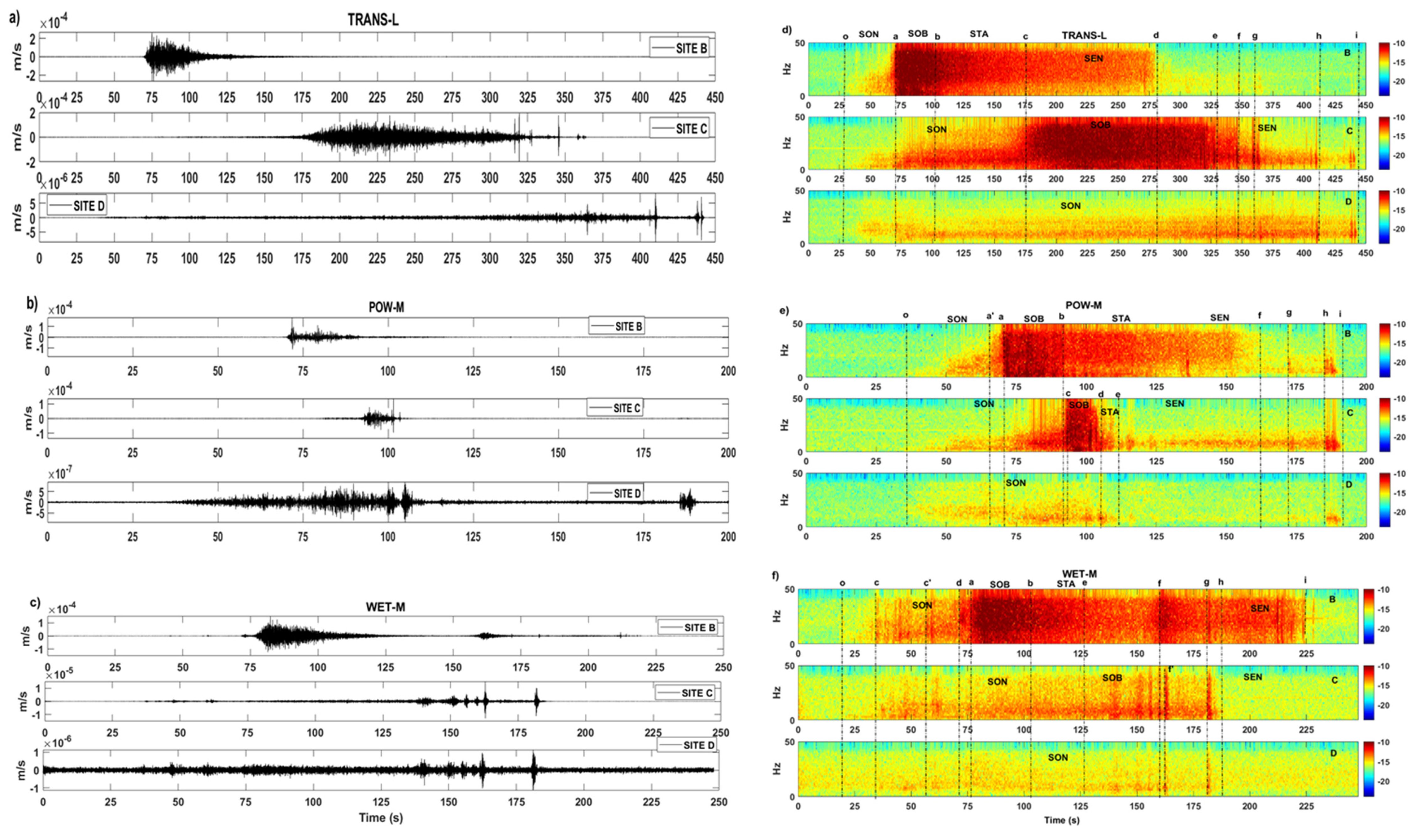
4. Avalanche Seismic Signal Evolution

One of the characteristics observed in the seismic signals of a single avalanche is their evolution in time and frequency content (spectrograms) along the avalanche path, reflecting the evolution of the flow at different elevations. Each avalanche type displays different patterns in the evolution of the seismic signal.
To illustrate the evolution of the flows along the path three representative avalanches each of a different type (Av4 TRANS-L (TRANS), Av5 POW-L (POW), and Av7 WET-M (WET)) were selected from the avalanches in Table 1. The time series of the final seismogram (FS) of these avalanches recorded at sites B, C, and D (Figure 1 and Figure 2) were displayed using a common time (top Figure 3, Figure 4 and Figure 5). The spectrograms were calculated and displayed in the same manner at the bottom of Figure 3, Figure 4 and Figure 5. Appendix B and Table A1 give a detailed explanation of the arrival times and outstanding features (OF) of the sections (SON, SBO, STA, and SEN) of the spectrograms, which are consistent with the images of the GEODAR [49]. Here, we highlight the most distinctive features of the signals of the three avalanche types. Note the differences in the duration of the signals as well as in the shape of each recording site and flow type. In the time series, note the shorter duration (150 s) of the powder-snow avalanche signals (POW, Figure 3) with respect the durations of the transitional avalanche (425 s) (TRANS, Figure 4) and of the WET avalanche (220 s) (Figure 5). The spindle-cigar shape in the time series referred to in the literature as a typical pattern of seismic moving sources, i.e., snow avalanches, debris flows, lahars, etc., [8,13,15,40,63,64] is more prominent in seismograms at sites C and D, located at some distance from the start of the avalanche, whereas wave packets of higher amplitudes are observed in the seismograms at B. Note that the sections of the spectrograms are different depending on the avalanche type and site. POW (Figure 3 and Figure A3e) and TRANS (Figure 4 and Figure A3d) avalanches show a clear SON section at B and C in contrast to the WET avalanche (Figure 5 and Figure A3f) in which the SON section is not clear since it shows peaks of energy associated with impacts. No specific SON section is observed at any of the three avalanches at D.
The SBO section in the POW avalanche is short at B (22 s) and at C (10 s), and no section is observed at D. The duration of this section in the TRANS avalanche at B is longer (35 s) than the section in the POW and the WET (28 s) avalanches. At C, in contrast to the POW avalanche, the SBO section in the TRANS avalanche is very long (173 s) and energetic. The SBO section in the WET avalanche is not very well observed at C and it is similar to the SBO section in the TRANS avalanche at D. No SBO section is observed at any of the three avalanches at D. The STA and SEN sections are longer in the WET (121 s) and TRANS avalanches (123 s) than in the POW avalanche (68 s) at B. This section is almost absent in the POW and the WET avalanches at C. In the TRANS avalanche, it disappears at the expense of the SBO section at C. The spectrogram in the TRANS avalanche at D is similar to that of the WET avalanche at C, showing mainly energy of low frequency content. Note, also, the energetic phase at the end of the signals observed in the three avalanches that corresponds to the stopping phase [22].
We obtained an average of the avalanche front speed between the two recording sites (B and C) by considering the time taken by the avalanche to travel from one site to the other (difference in the arrival time of the SBO sections) and the distance between the two sites (Table A1). This is possible if the avalanches reach the sensors. However, this condition is not always fulfilled.
To resolve this problem, we developed a method to quantify the SON section of the FS spectrograms in order to derive the speed of the avalanche front. We took advantage of the close link between the shape displayed by the SON sections of the spectrograms and the characteristics of the avalanche. Our analysis of hundreds of seismograms of diverse snow avalanches at the different sites provides robust evidence of this behavior.

5. Methodology and Quantification

5.1. Quantification of the Spectrogram SON Section

The increase in amplitudes of the frequencies in time in a quasi-exponential shape of the SON section of the spectrograms can be expressed as Equation (1)
F (t, f) = K (t, f) eβ (f, t) t
where F (with units of Hz) is a function that limits the amplitude of the spectrogram, which is a function of time, t(s), and frequency, f(s−1). K(s−1) and β(s−1) are functions that describe the shape of the spectrogram. To obtain Equation (1), following [65] we first deduced the equation of the decrease in the signal amplitudes A (t’, f) (m/s) at the sensor at a distance r(t’), in m, from the source (avalanche)
A (t’, f) = As (t’, f)/ (√ (2π h r(t’))) e − α(f) r (t’)
where
α (f) = π f/(Q(f)c(f))
Equation (2) considers the energy flux of the surface seismic waves through a cylindrical surface of radius r(t’), varying in time (t’) and height h (m) [16]. As (t’, f) (m2/s) is the amplitude at the source. t’(s) is time from the source. α (f) (m−1) is the intrinsic attenuation factor and the other term corresponds to the geometrical spreading. The ground seismic characteristics are involved in the ground quality factor, Q (f,), and in c(f) (m/s), the phase velocity of the surface waves. Equation (2) can be expressed as an exponential decreasing function
A (t’, f) = K (t’, f) e−β(f) t’
where r(t’) = S (t’) t’, S(t’) being the speed of the avalanche, in m/s,
β (f, t’) = α(f) S (t’)
and
K(t’, f) = As (t’, f))/√(2π h r(t’))
When a change of the time/distance reference is applied, Equation (4) becomes
A(t, f) = K(t, f) eβ(f, t) t
which is the same as Equation (1). t accounts for the change of reference in time (t = −t’). In this case, the origin of time and distances is the sensor instead of the source. Distances decrease as the avalanche approaches the sensor. In Equation (7) the amplitudes increase in time as in the spectrograms. Figure S3 in the supplementary material shows, as an example, a synthetic spectrogram using Equation (7). This figure reproduces the shape of the spectrograms.
To obtain parameters K and β of Equation (7), the Hough Transform (HT) [53] was applied to the spectrograms considered as an image. To this end, the amplitudes of the spectrogram (Figure 6a) were band-pass filtered in amplitudes (for all the times and the complete set of frequencies), selecting the range that was interesting to highlight (Figure 6b). The filtered image of the spectrogram was binarized to distinguish the arrival of the more energetic frequencies (Figure 6c). The binarized image was convolved with an edge detector mask [66] to highlight the lines of interest after a change of coordinates between the originals of the spectrogram (f, t) and those of the binary image (y, x). The HT was then applied to the final binary image (black and white) (Figure 6d), where the straight lines are defined by the limit of the white, the black corresponding to the background. Different fits defined by parameters Ai (slope) and Bi (y-intercept) were obtained through the application of the HT (Figure 6e) to each spectrogram. The averages of all the possible fits of Ai and Bi yield the slope, a, and the y-intercept, b, of
y(x) = ax + b
which allows us, after a change of variable, to obtain the functional relationship between time and frequency that limits threshold of amplitudes selected in the spectrogram
F(t) = a t + b
A relation between Equations (7) and (9) is necessary, i.e., between the coefficients K and β and a and b. However, an analysis of the dependence of the parameters in frequency is previously required. Note that the HT method uses a binarization process and that for each time HT discriminates the amplitudes to determine the shape of the SON section of the spectrogram by a threshold value. The dependence on frequency of β (f, t) (Equation (5)) is due to α(f), and not to r(t), which is not frequency dependent. The effect of the variation in distance r (t) leads to a variation in the amplitude values of the spectrogram in the same ratio for each time. As regards K (t, f) (Equation (6)), the same effect causes the dependence in r(t). Note that the dependence on f is through the source (As (t, f)). As a result, the amplitude ratio of the values for the threshold for each time (distance) does not change and does not affect the shape of the spectrogram detected by the HT method. Moreover, in Equation (2), an increase in amplitudes owing to the incorporation of snow as the avalanche approaches the sensor was neglected. The reason for this is that the increase in mass would affect the amplitudes at the same ratio for all frequencies at each time.
Following the above analysis, we may assume that K in Equation (7) is constant termed K’ in order to compare Equation (7) with Equation (9) yielding
A (t, f) = K’ eβ(f, t)t
To obtain the link between Equations (9) and (10), we apply the function ln to Equation (10) to its linearization
ln (A (t, f)) = ln K’ + β (f, t) t
Given that we are considering a threshold in the spectrogram amplitudes (upper limit) we impose Equation (12) on the implicit function Equation (11)
ln (A (t, f)) = Const.
As a result, Equation (13) is obtained which is a function that fulfills a fixed amplitude in the spectrogram
F’ (t) = ln K’ + β t
yielding to
F (t) =K’ eβt
The function of the frequency in time F(t) corresponds to the upper limit of the amplitude (Equation (14)) considered in the spectrogram.
The parallelism of the linear Equations (9) and (13) shows that the y-intercept term of the linear equation, b, has the role of ln K’ and the slope, a, has the role of β. Note that the spectrogram image is represented as a logarithmic function of the amplitudes. The identification of the left sides of Equations (9) and (13) is therefore correct. This comparison leads to β being frequency independent. This result is not inconsistent since the value of the slope, a, is obtained from the average of the different slopes of the fits to the spectrogram image.
The above process was applied to the SON section of the spectrogram of the final seismogram (FS) of the different avalanches recorded at sites B and C (Table 1). The extracted parameters κ i and βi (Equation (14)) for all the avalanches and sites are shown in Table 2.
Figure 7 and Figure 8 show the curves for Equation (14) of the SON section of the spectrogram of the avalanches for sites B and C, with the values in Table 2 to facilitate comprehension of these results. The curves are identified as in Table 1. Capital letters B or C are added to the avalanche name in accordance with the site. In these graphs, the errors are not considered to facilitate visualization. The curves were shifted in time to compare their curvatures. This shift corrects the different origins of time of the spectrograms in the image processing and does not affect the curvature.

5.1.1. Curves at B

Note that the curves are bunched, according to their avalanche type (Figure 7). The curves of the POW avalanches (in light blue) are steeper, showing a sharp increase in frequency greater than that of the TRANS (in light purple) and especially the WET (in light brown) avalanches. Note that the behavior of Av10B POW-M differs from that of the other POW avalanches, being more similar to that of WET avalanches. This behavior will be considered in the discussion. Curves for WET avalanches present a gentler increase in frequency with time. A comment regarding avalanches Av11B TRANS-L and Av12B WET-L defined as transitional and wet, respectively, in the classification in [19] is opportune. The behavior of Av11B TRANS-L is closer to that of the wet avalanches, whereas Av12B WET-L has a shape similar to that of the transitional avalanche Av4B TRANS-L. In the discussion this discrepancy in behavior with respect to their classification will be considered.

5.1.2. Curves at C

At this location, the POW curves (in dark blue) are bunched including Av10C POW-M (Figure 8). The curvatures of Av11C TRANS-L and Av12C WET-L are similar to those of the POW avalanches, differing from that of the transitional avalanche (Av4C TRANS-L, in dark purple), which has a gentler curvature. The curves of the WET avalanches (in dark brown) are gentler than those of the other avalanche types. As for Avalanche Av10 POW-M, while the behavior at B differs from that of the POW avalanches, its behavior coincides at C. This behavior will be considered in the discussion. Although the WET avalanches do not reach sensor C (Table 1), we regard the values obtained as correct because the coefficients correspond to the SON section when the avalanche does not reach the sensor.

5.1.3. Evolution of Curves from B to C

We now focus our attention on the evolution of the avalanches from sites B to C. Since the figure of all the curves at B and C plotted jointly is confusing, the curves are presented according to the avalanche type. Figure 9 corresponds to powder avalanches. Note that the curves are gentler at C than at B, maintaining the two groups apart. Figure 10 shows the curves of the transitional avalanches recorded at B and C. Curves of avalanche Av12 WET-L are included in the plot because the curvatures at sites B and C are similar to those of the TRANS avalanches. Figure 11 corresponds to the curves of wet avalanches recorded at B and C. In general, the curvature of the curves at B and C are fairly similar.

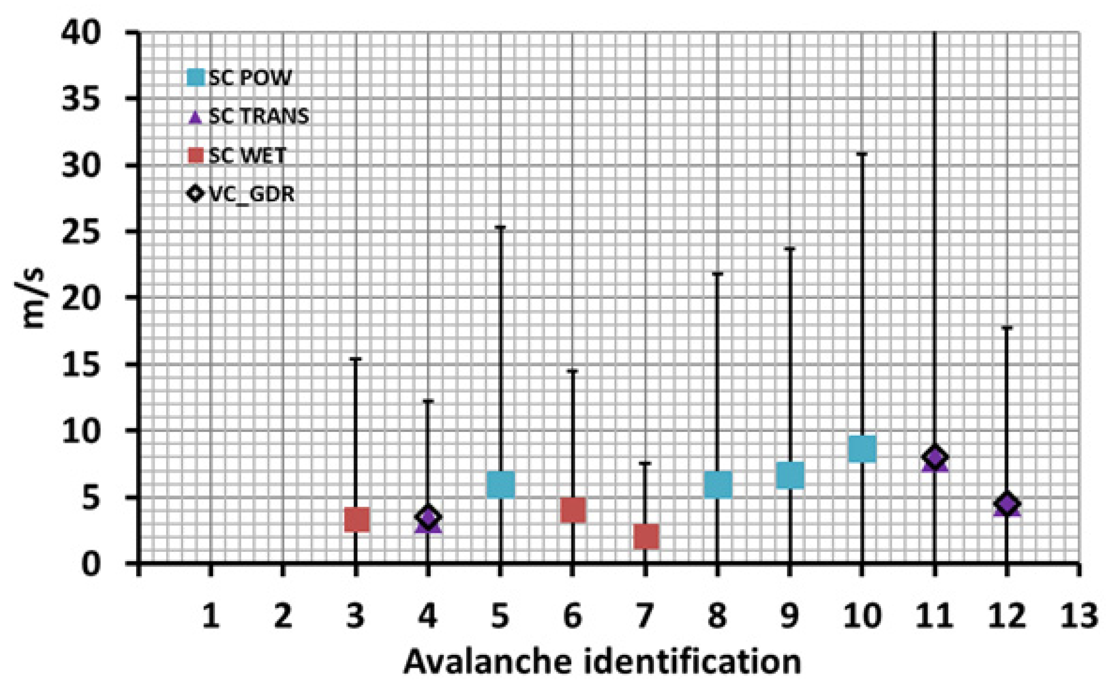
5.2. Avalanche Speed Estimation

Equation (5) allows us to estimate the speed of the front of the avalanche (S) using the β(s−1) values obtained for each spectrogram. However, the parameter α(m−1) depends on the seismic characteristics of the ground (Equation (3)). In the absence of measured values of α, there is an extensive debate about how to fix this value. Different authors have assumed that α (m−1) is either constant or dependent on the frequency, e.g., [16,67,68,69]. This selection is crucial for the calculation of the energy released by a mass in movement. The choice of α has also repercussions in the calculation of the speed of the avalanche (Equation (5)). In the specific case of VdlS, no values of α (m−1) are known, although attenuation parameters κ (s−1) (spectral decay factor) in the Swiss territory have been calculated [70], even if they are not the same. To resolve the absence of α values, a procedure was adopted to determine them in order to estimate the avalanche speed (S). Figure 12 shows a diagram of the procedure. To fix α from the calculated βi (from HT), we took advantage of the estimates of the avalanche velocity (VGDRi), obtained from the GEODAR system [30,48,49]. This velocity is defined as the ground-parallel velocity down the talweg in [30] and it is the projection of the velocity along the path similar to our speeds (S). We maintain below this difference (speed S (obtained from seismic) and velocity VGDR (derived from GEODAR)) in order to facilitate comprehension. Note that both values are not derived from a direct measurement. We used, when available, the avalanche velocity values (VGDRi). In fact, we focused our attention on the values corresponding to the few seconds before the avalanche reached the sensor. In other words, we considered the velocities (VGDR) corresponding to the SON section of the avalanche. We assumed an error of 10% in our visual determination from the GEODAR curves. The αi values were calculated from the βi values obtained from HT for each avalanche and for each site (B and C) using Equation (5) (Figure 12). To estimate the speed of the avalanches, we took the average, αa, obtained from the different αi for the two sites (Table 3). We obtained different values αa for sites B (0.004 ± 0.001 m−1) and C (0.010 ± 0.023 m−1), the values being higher at C than at B (Table 3). In this calculation, avalanches.
Av11C TRANS-L and Av12C WET-L were ignored because they do not meet our requirements. We also calculated the median, αm. Given that the difference was not significant when considering the errors, we maintained αa for the calculations. The avalanche speeds S were obtained using αa and Equation (5) for the βi values (Figure 12). The speed values for both sites (SBa and SCa) and the values derived from VGDR, when available, are given in Table 3. Some velocity (VGDR) values at C are absent because GEODAR signal stops before reaching the range where the seismic sensor is located.
Likewise, some values are absent at B since the GEODAR signal does not provide images of the start of the avalanche [53]. This is a limitation of the triggering system. As mentioned above, our seismic recording system does not depend on the VdlS triggering system, thereby enabling us to obtain the entire avalanche signal.

6. Discussion

6.1. Avalanche Evolution

The spectrograms of the seismic signals (FS) of the three types of avalanche present differences along the path. In the POW avalanche (Figure 3), the arrival times of the wave packets in the signals at the three sites are closer together, whereas in the TRANS (Figure 4) and WET avalanches (Figure 5) the arrival times are spaced out. The SBO section of the TRANS avalanche is longer than that of the POW avalanche at C, although at B it presents a similar duration. This is not observed in the WET avalanche (Figure 5) in which the spectrogram at C is similar to that of the TRANS avalanche at D.
Moreover, each signal has several wave packets that arrive at different times (Figure 3, Figure 4 and Figure 5) depending on the velocity of the avalanche and on the internal surges or parts of the avalanche moving behind the avalanche front [19]. As mentioned earlier, a TRANS avalanche is a POW avalanche that evolves into a WET avalanche along the path and, in principle, TRANS avalanches have no specific rheology. The specific characteristics of the spectrograms allow us to distinguish between the different avalanche types given that the sections appear at different locations (and times) along the path (note the difference in the SBO section at C in both avalanches (TRANS and WET) and the similarity of the spectrograms at D (for TRANS) and C (for WET)). In contrast to the TRANS avalanche, the POW avalanche does not incorporate snow that produces energetic seismic signals from B to C. The effect of the incorporation of snow from B to C in the WET avalanche is insignificant in the spectrogram, and the flux (reflected by the spectrogram) at C is similar to that at the end of the TRANS avalanche at D. The examples presented show that the entire spectrogram of the seismic signals reflects the avalanche type and its evolution characteristics along the path, always in accordance with the perspective of the seismic signal analysis.

6.2. Averaged Curves

Although the majority of the curves constructed with the κ’ and β values obtained when applying our method agree with their avalanche type, the curves of Av10B POW-M, Av11B TRANS-L, and Av12B WET-L do not follow the general trend. A possible explanation for the behavior of Av10B at B could be that this avalanche, as reported in [19], was not released exactly in CB1 (in Pra-CB1, Figure 1). Given that it descended Gully 1 (Figure 1) as did the other avalanches reaching C, it presents the same behavior as the other POW avalanches at C. The Av11 TRANS-L and Av12 WET-L avalanches at C display a behavior akin to that of the POW avalanches (Figure 8), whereas at B the former acts as a WET avalanche while the latter behaves as a TRANS avalanche (Figure 7). The different starting zone of these avalanches (the release area was CB1 + CB2, Table 1) could give rise to a different state of the avalanche flow regime, resulting in a discrepancy in the behavior of the curves with respect to the other curves.
To deepen our understanding of the avalanche evolution, we calculated the mean values βm and K’m of the parameters according to the avalanche type and site in Table 2 (Table 4). We did not consider Avalanches Av10 POW-M and Av11 TRANS-L and Av12 WET-L so as not to alter the results because they do not meet our requirements. Although the errors are considerable with respect to these values, information on the evolution can be extracted from them. The average value of the exponent βm and K’m differ according to the avalanche type. For cavern B, situated upslope, the value of βmB for the POW avalanches is higher than that for the TRANS avalanches, which is in turn higher than that for the WET avalanches. This order is inverse for K’mB. As for site C, situated 920 m downslope, the βmC value for the POW avalanches exceeds those of the TRANS avalanches and WET avalanches.
The behavior of K’mC values is similar to that of K’mB values. Given that there is only one valid transitional avalanche at C, it is meaningless to draw conclusions on transitional avalanches from Table 4. Conclusions similar to those of the individual avalanches may be drawn for the three avalanche types and their evolution from B to C. The ratio between the exponents defined as index E= βmCmB (Table 4) provide us with an index of the evolution of the avalanches between the two sites. A value of E close to 1 indicates an absence of evolution of the avalanches from B to C. Thus, index E indicates a higher evolution from B to C for the SON section of the powder avalanches than for the wet avalanches. Figure 13 displays the curves for the averaged values at B (Figure 13a) and C (Figure 13b) and the evolution from B to C for POW (Figure 13c), TRANS and WET (Figure 13d) avalanches in order to facilitate visualization. Figure 13d shows that the evolution from B to C is more marked in TRANS avalanches than in WET avalanches. The curve of the TRANS avalanche is close to that of the POW avalanches (Figure 13a) at B, whereas at C the curve is close to that of the WET avalanches (Figure 13b). Note that although TRANS and WET avalanches at C show a similar behavior in the SON section, the differences in the spectrograms (mainly in the SBO section (Figure 4 and Figure 5)) indicate differences in the flow regime.

6.3. Front Avalanche Speed Estimation

Table 3 shows the front avalanche speeds for both sites (SBa and SCa) using αa and the values deduced from VGDR. Note that although the errors are large, the speed values deduced from the HT are, in general, close to the values of the avalanche velocities (VGDR) derived from GEODAR data. There is, however, a discrepancy between the values of the velocity deduced from our calculations and the speeds derived from GEODAR measurements for POW avalanches. At B, the speeds are generally higher than the velocities deduced from GEODAR, whereas at C this is the inverse. A comparative study of the spectrograms and GEODAR images concerning the difference of the arrival times of the energy reveals that the GEODAR images and the seismic signals do not reflect the same phenomenon [31]. This agrees with the assertion that GEODAR only detects the denser flow structures below the diluted powder cloud [30], and also with the fact that the entrainment of the powder part of the avalanche generates seismic signals [19,57]. Therefore, the use of the two complementary measurement systems is useful. However, this needs to be corroborated in future studies. Bearing this in mind, a second more realistic attempt was made to calculate the avalanche speeds. The elimination of the αi values of the POW avalanches to calculate an averaged value, αe, of this seismic ground property is reasonable if GEODAR and seismic signals do not reflect the same phenomenon in POW avalanches. Thereafter, we obtained the averaged value αe using the procedure indicated in Figure 12, excluding POW avalanches, and Av11C TRANS-L and Av12C WET-L avalanches. The values obtained were 0.0025 ± 0.0015 m−1 for site B and 0.015 ± 0.038 m−1 for site C (Table 3). Although it seems that the procedure of obtaining α (Figure 12) is circular, this is the only one we are able to follow in the absence of real seismic characteristics of the ground. The αe values for sites B and C (Table 3) are of the order of the values derived from other studies, e.g., [16,66,69]. These values yield a quality factor Q (f) (Equation (3)) for the same frequency and phase velocity that is higher at B than, downslope, at C. This result is plausible since the seismic characteristics of the two sites are different (geological effects and snow-cover e.g., [25,57]) with the result that this difference is reflected in the calculated αa.
In Figure 14 and Figure 15, the speed values SBap and SCap (Table 3) for the different avalanche types are plotted jointly with the velocities derived from GEODAR (VGDR) when available for sites B and C. Using this αe, the coincidence of the speed values with the velocities derived from GEODAR is higher for TRANS and WET avalanches. The agreement of the values of the TRANS avalanches for the two types of measurements is satisfactory at C. The speed values obtained for POW avalanches are plotted in the figures, but are not compared with the VGDR values for the reason explained above. In Figure 16, the speed values at B and C are plotted for TRANS and WET avalanches, with their averaged values. Although the standard deviations calculated with the errors in Table 3 are very high, the averaged values yield information that merits a comment. The averaged value of the front speed for TRANS avalanches is 42 ± 3 m/s (deviation corresponds to the averaged value) at B. Note that the front speed value of the Av12 WET-L at B is similar to that of the TRANS avalanches. The averaged value of the front speed for WET avalanches is 23 ± 7 m/s at B. This value is similar to that obtained for the Av11 TRANS-L. The speed values of the aforementioned avalanches were calculated using the αe value (equation 5) with the result that the speed values of these avalanches are consistent with the behavior of the corresponding curves. At C, the speed values for the two types of avalanche are similar within the range of (3–8) m/s with an average speed value of 4 ± 4 m/s. The speed values at B are higher and more dispersed than those at C. In both types of avalanche, a decrease in the speed is observed, the decrease being greater for TRANS avalanches than for WET avalanches. At site C, no values of GEODAR velocities for WET avalanches exist because the avalanches stopped before reaching the site as indicated by the images [49]. Although WET avalanches 6 and 7 (Figure 15) did not reach sensor C (Table 1), we maintained the speed values because, as mentioned above, the SON section corresponds to waves travelling before the avalanche reaches the sensor.

7. Conclusions

The division into sections (SON, SOB, and STA-SEN) of the spectrograms of the seismic signals generated by snow avalanches is useful to obtain information about avalanche behavior. These sections differ in duration, amplitude, and frequency content according to the avalanche type, and provide detailed information of their evolution along a path.
The application of the Hough Transform to the spectrograms when considered as an image allows us to parameterize the shape of the SON section and deduce the avalanche front speeds. Anaelastic attenuation coefficients, α(m−1), were obtained for two sites at VdlS. These coefficients characterize these sites seismically and can be used in further studies in the absence of values obtained from specific experiments.

Supplementary Materials

The following are available online at https://www.mdpi.com/2076-3263/10/3/113/s1, Figure S1: Schemes of the coordinate system matrix rotations. Figure S2: Scheme of the creation of the component SF of the seismic record. Figure S3. Synthetic spectrogram using Equation (7).

Author Contributions

Conceptualization, E.S; methodology, E.S. and E.L.F.-M.; software, E.S., E.L.F.-M., P.R.-L. and M.T.; validation, E.S., E.L.F.-M., P.R.-L., M.T. and G.F.; formal analysis, E.S., E.L.F.-M., P.R.-L. and M.T.; investigation, E.S., E.L.F.-M., P.R.-L., M.T. and G.F.; resources, E.S. and E.L.F.-M.; data curation, E.S., M.T. and P.R.-L.; writing—original draft preparation, E.S.; writing—review and editing, E.S., E.L.F.-M., G.F. and P.R.-L.; visualization, E.S.; supervision, E.S.; project administration, E.S.; funding acquisition, E.S. and E.L.F.-M. All authors have read and agreed to the published version of the manuscript.

Funding

This research was funded by the CHARMA (CGL2013–40828–R) and the PROMONTEC projects (CGL2017-84720-R) of the Spanish Ministry of Economy, Industry and Competitiveness (MINEICO-FEDER) and RISKNAT group (2014GR/1243. The first two authors (ELF-M and ES) acknowledge a grant from the Instituto de Geofísica, UNAM, México. PRL received a pre-doctoral grant (FI-DGR2016) from AGAUR, Secretaria d’Universitat i Recerca del Departament d’Economia i Coneixement, Generalitat de Catalunya.

Acknowledgments

The authors wish to thank our colleagues of the UB avalanche Team (RISKNAT) for their assistance in the field campaigns. The authors are indebted to the SLF dynamics team and logistics staff for their help in the installation of the instruments and field experiments. We are grateful to A. Khöler for his introduction on the interpretation of the GEODAR measurements. Special thanks are due to C. Pérez-Guillén for her contribution to the discussion on snow avalanches and to the methodology. The useful comments of two anonymous reviewers helped us to improve this manuscript.

Conflicts of Interest

The authors declare no conflict of interest. The funders had no role in the design of the study; in the collection, analyses, or interpretation of data; in the writing of the manuscript, or in the decision to publish the results.

Appendix A. Seismic Signal Transformation

Appendix A.1. Seismic Signal in the Slope Direction Transformation

The seismic amplitude in the slope direction is obtained by applying a matrix rotation R1(ϕ) around the E-W axis to the seismic components of the vector ground u(uN-S, uE-W, uZ, t) (ui(t), i = 1, 2, 3)), where ϕ is the slope of the ground where the sensor was installed and the signal recorded (Figure S1a)
u(uY’(t), uE-W(t), uNo(t)) = R1(ϕ) u(uN-S(t), uE-W(t), uZ(t))t
As a result, the two components of the vector in the vertical plane (N-S, Z) are orthogonal to the slope direction (No) and in the slope (Y´) direction, respectively (Figure S1a). The amplitude in the seismic component in E-W direction is not altered. A second rotation matrix of R2 (θ), where θ is the direction of the flow with respect to the N-S direction is applied to the vector in the plane (Y’,E-W) to obtain the amplitude in the direction of the flow and orthogonal to the slope.
u(uS(t), uST(t), uNo(t)) = R2(θ) u(uNo(t), uY’(t), uE-W(t))t
In Figure S1b a detail of the second rotation is shown to derive u(uS(t), uST(t), uNo(t)). Figure A1 shows an example of the result of the application of the rotations for the three types of avalanche. Note that the amplitudes are equally distributed in all the components for each avalanche.

Appendix A.2. Seismic Signal in Polar Coordinates Transformation

Once matrix rotation R1(ϕ) (Equation (A-1)) is applied to the seismic components of the vector ground u(uN-S, uE-W, uZ, t) (ui(t), I = 1,2,3)), to obtain u (uY’(t), uE-W(t), uNo(t)) (Figure S2a) a second matrix rotation R2(ξ (t)) is applied to the two components (Equation (A-3)).
u(uR(t), uT(t), uNo(t)) = R2(ξ (t)) u(uY’(t), uE-W(t), uNo(t))t
The R(t) direction corresponds to the projection of the vector u(t) in the plane (Y’, E-W), which is orthogonal to No (Figure S2b). Note that the rotation matrix R2 (ξ (t)) varies in time, depending on the instantaneous direction ξ(t) (ranging [0° to 360°]) of the ground particle movement vector in the plane (Y’, E-W), which is orthogonal to No. The values of the angle ξ (t), which corresponds to the azimuthal angle in Spherical coordinates, were obtained considering the components uY’(t) and uE-W(t) (Figure S2b).
After applying the rotation matrix R2 (ξ(t)), the whole seismic amplitude of the vector u(t) is contained in the plane defined by No and the R(t) (Figure S2b) and split into these directions. Finally, the radial component r(t) (or FS amplitude) and the polar angle e(t) (ranging [90°to−90°]) were obtained from the uNo(t) and the instantaneous uR(t) components. As a result, the initial vector u(t) in the seismic components (Cartesian coordinates) [uN-S, uE-W, uZ, t] is expressed as [r, ξ, e, t] after the transformation to Spherical coordinates; r(t) corresponds to the Final Seismic signal (FS). Figure A2 shows the results of the different steps of the transformations for a SON section signal.
Figure A1. Example of the result of the application of the rotations R1 and R2 to the SON section for the three types of avalanche (a) TRANS, (b) POW, (c) WET. Left: time series. No direction normal to the slope; Slope: in slope direction; Tslope: orthogonal to No and slope directions. Vertical axis in time series corresponds to the ground movement generated by the avalanche in m/s. Horizontal axis is time. Right: Spectrogram amplitudes (in color) in 10−1dB. Vertical axis in the spectrograms corresponds to frequency in Hz. Horizontal axis is time.
Geosciences 10 00113 g0a1

Appendix B

A detailed description of the seismograms and spectrograms of avalanches Av4 TRANS-L (TRANS), Av5 POW-L (POW), and Av7 WET-M (WET) presented in Section 4 (Figure 3, Figure 4 and Figure 5) is offered here. The different sections (SON, SBO, STA, and SEN) of the seismic signal are indicated. Table A1 indicates the different arrival times and outstanding features (OF) mentioned in the text. In this appendix the three avalanches are presented together in Figure A3 for comparison. In this description, we refer to the GEODAR images that can be accessed in [49] for comparison. The ranges of 1300 m and 600 m in the GEODAR images correspond to the location of the seismic sensors at B and C.

B.1. Transitional Avalanche (TRANS)

Figure A2. Example of the result of the application of the rotations to the SON section of an avalanche. (a) Time series the original seismic components (Z, N-S, E-W). (b) Time series after application of R1(ϕ) in (No, Y’ and E-W components. (c) Time series after application of R2 (ξ(t)) in No, R, and T components. (d) Time series (up) and spectrogram (down) of FS, result of the representation in polar coordinates. Vertical axis in the time series ground movement in m/s. Horizontal axis time in s. Spectrogram amplitudes (in color) in 10−1dB.
Geosciences 10 00113 g0a2
This avalanche was studied and defined as a typical transitional one [48]. Figure A3a,d show the time series and spectrograms of the seismic records obtained at B, C and D. In the time series, the duration of the energetic parts is 60 s at B, which shows two internal surges of maximum amplitudes at 75 s and 85 s. At C, at a distance of 690 m from B, the energetic part of the seismic signal presents a cigar shape with a duration of 150 s with a gradual arrival of the front at approx. 175 s when the amplitudes at B are attenuated. At D, at a distance of 525 m from C, the signal, with amplitudes of one order of magnitude lower, is longer than the previous ones with a duration of approx. 400 s, showing peaks at its end at approx. 350 s and 412 s. The representation of the seismic signals in the frequency domain (spectrograms) (Figure A3d) enhances the information contained in the time series. Note that the information of the signals is more detailed, especially the duration of the parts with higher seismic amplitude. The different sections of the spectrograms (SON, SOV (SBO, STA), SEN) described in earlier studies [18,31,57] are visible and the intervals when the avalanche is over the sensors (SOV sections) are well determined. Outstanding features (OF) in the spectrograms (Figure A3d) are indicated by letters and are included in the following explanation. Table A1 shows the arrival times corresponding to these features. The SBO section starts at 70 s (a) at B, which represents the arrival of the avalanche front at the sensor (Figure A3d). The avalanche flows over B for 35 s (a-b). Section SON (o-a) has a duration of 38 s (Table A1 and Figure A3d). The SEN section ends at 278 s (d) (Figure A3d). The total duration of the avalanche signal (a-d) at B is 208 s. Seismic amplitudes are observed albeit with very low values up to (d). This corresponds to the avalanche descending the path as observed at C. The avalanche reaches C at 175 s (c), and flows over it (SBO) for 153 s (c-e) or even longer (173 s, c-f). Note that the SBO section at C is longer than that at B because of the decrease in the speed of the flow in the runout zone and because of a possible increase in the avalanche size due to snow entrainment. At sensor D, which is located on the opposite slope, the seismic amplitude is observed only at low frequencies [5,6,7,8,9,10,11,12,13,14,15,16,17,18,19,20,21,22,23,24,25,26,27,28,29,30,31,32] Hz with lower amplitude than at sensors B and C. This is due to the attenuation of the seismic amplitudes with distance since the flow mass stopped at 425 m from sensor C at a considerable distance from sensor D (Figure 1 and Figure 2). This information is consistent with that from the GEODAR image (GEODAR-2013-02-01-17-14-50-MTI.pdf in [49]). Markers (a) and (c) correspond to the time when the avalanche mass is in the range of the sites B (1300 m at 23 s) and C (600 m at 130 s) of the GEODAR image. The average speed of the avalanche from its starting area (CB1) to B is 26 m/s.
Figure A3. Time series (left) and spectrograms (right) of the final seismogram (FS) shown with a common time for avalanches (a,d) TRANS), (b,e) POW and (c,f) WET (Table 1) recorded at sites B, C and D (Figure 1 and Figure 2) displayed with a common time in s (horizontal axis). Vertical axis in time series corresponds to the ground movement generated by the avalanche in m/s. Vertical axis in the spectrograms corresponds to frequency in Hz. Spectrogram amplitudes (in color) in 10−1dB. The sections and the OF indicated in Table A1 are marked in the spectrograms.
Geosciences 10 00113 g0a3
In this estimate, we considered the duration of the SON section (assuming that the start of the SON section coincides with that of the avalanche) and 985 m for the distance between the sensor and the avalanche-starting point. An average value of 6.6 m/s was obtained for the average avalanche speed from B to C. To this end, we considered 690 m to be the distance between these two sites and the difference in the arrival times of the SBO sections (Table A1). The total duration of the SON section (o-c) at C is 143 s. The amplitudes observed at C for times exceeding 326 s (e-f and up to (g) and (h)), indicating that no mass is over this sensor, correspond to the flux of the mass around 400–300 m range at approx. 312 s from the start of the aforementioned GEODAR image. It is important to highlight the abrupt end of the signal ((f), (g), and (h)) accompanied by the sudden increase in amplitude observed at the end of the spectrograms at C and D. This corresponds to the stopping phases aforementioned ([22], Figure 3 in [30]). The end of the avalanche is shown in the above mentioned GEODAR image of this avalanche at the range of 200 m (387 s), which indicates that it does not reach D. This confirms the observation in the spectrogram of sensor D. The scarce seismic amplitudes detected with low frequency content correspond to attenuated seismic waves transmitted into the ground from the avalanche.

B.2. Powder-Snow Avalanche (POW)

Figure A3b,e show the time series and spectrograms of a powder–snow avalanche (POW) recorded in the sensors at sites B, C, and D. Table A1 shows the arrival times of the OF. At sites B and C, the time series show wave arrivals of durations 25 s (in B) and 12 s (in C). The signal at D is longer than at B and C, albeit two orders of magnitude smaller, with a spindle shape with peaks around 185 s. The SON section (o-a) in the spectrogram at B has a duration of 34 s. The duration of the SBO section (a-b) at B is 22s. After (b) amplitudes are observed for 68s up to (f). These correspond to the SEN section. The start of the SBO section at C (c) is at 93 s, leading to an average avalanche speed of 30 m/s between B and C. The start of the SBO section at C (c) indicates that when the avalanche body reaches C, it has already passed over B (b). Additionally, the duration of the SBO section at B (a-b, 22s) is longer than that at C (c-d, 10 s), which suggests that the avalanche has reduced its mass. Note that practically no STA section is observed at C. As in the TRANS avalanche, seismic amplitudes are observed at C after (d) and up to (i), when the mass is not over the sensor. These correspond to the flux of the mass around the range 1000 m as observed in the GEODAR image (2013-02-05-23-31-53- MTI.pdf in [49]) (possibly related to lateral moving masses whose signals are projected along a line). In this avalanche, the signal (stopping phase) at 178 s, denoted by (h) in the spectrograms of the three sites, corresponds to the stop of the avalanche observed in the GEODAR image.

B.3. Wet-Snow Avalanche (WET)

Figure A3c,f show the time series and spectrograms of this WET avalanche recorded in the sensors at sites B, C and D. The total duration of the avalanche is approx. 200 s, longer than that of the POW avalanche, but shorter than that of the TRANS avalanche. In the time series at B, the duration of the seismic amplitudes is approx. 50 s. At C and D this is of one order of magnitude lower and the seismic amplitudes are scarcely visible when it is observed at B. However, after this time, peaks are present, coinciding in time at C and D (Figure A3c). In the spectrogram at B, the SON section (o-a) lasts 57 s. The SOV (SBO and STA) section (a-e) at B lasts 51 s. The seismic amplitudes observed in the spectrogram at B in section SBO (a-b) coincide in duration with the signal observed at the range 1300 m in the GEODAR image (2013-04-14-22-49-51-MTI.pdf in [49]). The distribution of amplitudes in the spectrogram at C indicates that the avalanche has not reached this site. The point where the avalanche stopped coincides with the vanishing of amplitudes in the spectrogram at C (h) preceded by a peak (g), which corresponds to the stopping phase. Although the seismic amplitudes are very low at D, the spectrogram reproduces the peaks at C. A stopping phase (i) is also observed at B. Note that peaks in the SON section at B, C (and D) are present, which indicates the presence of surges at the beginning of the avalanche. This is not possible to confirm from the GEODAR image since it starts later. Because of the surges observed at B and because the avalanche does not reach the sensors at C and D, it is not possible to estimate the speed of this avalanche. This information is consistent with that of the aforementioned GEODAR image, which indicates that the avalanche stopped at range 950 m (h) 135 s from the start of the image.
Table A1. Arrival times and duration of the outstanding features (OF) in Figure A3. In bold sections mentioned in the text.
TRANS- L POW- M WET-M
OFTime
(s)
DURATION (s)Av. Speed (m/s) OFTime
(s)
DURATION (s)Av. Speed (m/s) OFTime
(s)
DURATION (s)Av. Speed (m/s)
SON_Bo32o-aSON (o-a)SON_Bo36o-a SON (o-a)SON_Bo19o-dSON (o-a)
3826 a’663429 c345217
a-cB-C a-cB-C c’57o-a
1056.6 2330 d7157
SOB_Ba70a-b SOB_Ba70a-b SOB_Ba76a-b
35 STA_Bb9222 28
a-d b-f STA_Bb104a-e
208 SEN_Bf16068 e12751
STA_Bb105o-d a-h f159
246 g171114 o-i
d-b o-h 206
SEN_Bd278173 h184148 END_Bi225b-i
i191o-i SEN_B 121
SON_Co32o-c 155
143 SON_Co19o-h
a-c SON_Co36o-c 167
105 57 STA_Cf’163
SOB_Cc175c-e SOB_Cc93c-d g181a-i
153 d10310 h186149
STA_Ce328c-f STA_Ce110d-e
f348173 7 SON_Dc34
g358c-g g171 STA_Df’163
183 SEN_Ch184e-h g181
h410c-i i19174
SEN_Ci441266 o-i
o-i 155
409
SON_Do32o-i SON_Do36o-e
h410409 e11074
SEN_Di441 h184

References

  1. Lawrence, W.S.; Williams, T.R. Seismic signals associated with avalanches. J. Glaciol. 1976, 17, 521–526. [Google Scholar] [CrossRef] [Green Version]
  2. Salway, A.A. A Seismic and Pressure Transducer System for Monitoring Velocities and Impact Pressure of Snow Avalanches. Arct. Alp. Res. 1978, 10, 769–774. [Google Scholar] [CrossRef] [Green Version]
  3. Shaerer, P.A.; Salway, A.A. Seismic and impact-pressure monitoring of flowing Avalanches. J. Glaciol. 1980, 26, 179–187. [Google Scholar] [CrossRef] [Green Version]
  4. Firstov, P.; Sukhanov, L.; Pergement, V.; Rodionovskiy, M. Acoustic and seismic signal from snow avalanches, Transactions (Doklady) of the U.S.S.R. Acad. Sci. Earth Sci. Sect. 1992, 312, 67–71. [Google Scholar]
  5. Norris, R.D. Seismicity of Rockfalls and Avalanches at Three Cascade Range Volcanoes: Implications for seismic Detection and hazardous Mass movements. Bull. Seismol. Soc. Am. 1994, 84, 1925–1939. [Google Scholar]
  6. Leprettre, B.; Navarre, J.-P.; Taillefer, A. First results from a pre-operational system for automatic detection and recognition of seismic signals associated with avalanches. J. Glaciol. 1996, 42, 352–363. [Google Scholar] [CrossRef] [Green Version]
  7. Suriñach, E.; Furdada, G.; Sabot, F.; Biescas, B.; Vilaplana, J.M. On the characterization of seismic signals generated by snow avalanches for monitoring purposes. Ann. Glaciol. 2001, 32, 268–274. [Google Scholar] [CrossRef] [Green Version]
  8. Van Herwijnen, A.; Schweizer, J. Monitoring avalanche activity using a seismic sensor. Cold Reg. Sci. Technol. 2011, 69, 165–176. [Google Scholar] [CrossRef]
  9. Van Herwijnen, A.; Schweizer, J. Seismic sensor array for monitoring an avalanche start zone: Design, deployment and preliminary results. J. Glaciol. 2011, 57, 267–276. [Google Scholar] [CrossRef] [Green Version]
  10. Hammer, C.; Fäh, D.; Ohrnberger, M. Automatic detection of wet-snow avalanche seismic signals. Nat. Hazards 2017, 86, 601–618. [Google Scholar] [CrossRef]
  11. Heck, M.; Hammer, C.; Van Herwijnen, A.; Schweizer, J.; Fäh, D. Automatic detection of snow avalanches in continuous seismic data using hidden Markov models. Nat. Hazards Earth Syst. Sci. 2018, 18, 383–396. [Google Scholar] [CrossRef] [Green Version]
  12. Heck, M.; van Herwijnen, A.; Hammer, C.; Hobiger, M.; Schweizer, J.; Fäh, D. Automatic detection of avalanches combining array classification and localization. Earth Surf. Dyn. 2019, 7, 491–503. [Google Scholar] [CrossRef] [Green Version]
  13. Lacroix, P.; Grasso, J.-R.; Roulle, J.; Giraud, G.; Goetz, D.; Morin, S.; Helmstetter, A. Monitoring of snow avalanches using a seismic array: Location, speed estimation, and relationships to meteorological variables. J. Geophys. Res. 2012, 117, F01034. [Google Scholar] [CrossRef] [Green Version]
  14. Heck, M.; Hobiger, M.; van Herwijnen, A.; Schweizer, J.; Fäh, D. Localization of seismic events produced by avalanches using multiple signal classification. Geophys. J. Int. 2018, 216, 201–217. [Google Scholar] [CrossRef]
  15. Pérez-Guillén, C.; Tsunematsu, K.; Nishimura, K.; Issler, D. Seismic location and tracking of snow avalanches and slush flows on Mt. Fuji, Japan. Earth Surf. Dyn. 2019, 7, 989–1007. [Google Scholar] [CrossRef] [Green Version]
  16. Vilajosana, I.; Khazaradze, G.; Surinach, E.; Lied, E.; Kristensen, K. Snow avalanche speed determination using seismic methods. Cold Reg. Sci. Technol. 2007, 49, 2–10. [Google Scholar] [CrossRef]
  17. Vilajosana, I.; Suriñach, E.; Khazaradze, G.; Gauer, P. Snow avalanche energy estimation from seismic signal analysis. Cold Reg. Sci. Technol. 2007, 50, 72–85. [Google Scholar] [CrossRef]
  18. Vilajosana, I. Seismic Detection and Characterization of Snow Avalanches and Other Mass Movements. Ph.D. Thesis, Universitat de Barcelona, Barcelona, Spain, 2008. [Google Scholar]
  19. Pérez-Guillén, C.; Sovilla, B.; Suriñach, E.; Tapia, M.; Köhler, A. Deducing avalanche size and flow regimes from seismic measurements. Cold Reg. Sci. Technol. 2016, 121, 25–41. [Google Scholar] [CrossRef]
  20. Sabot, F.; Martinez, P.; Suriñach, E.; Olivera, C.; Gavalda, J. Detection Sismique Appliquée A la Caracterisation des Avalanches. In Les Apports de la Recherche Scientifique A la Sécurité Neige, Glace et Avalanches; Editions ANENA- CEMAGREF; Éditions Quae: Grenoble, France, 1995; pp. 19–24. [Google Scholar]
  21. Sabot, F.; Naaim, M.; Granada, F.; Suriñach, E.; Planet-Ladret, P.; Furdada, G. Study of the avalanche dynamics by means of seismic methods, image processing techniques and numerical models. Ann. Glacial. 1998, 26, 19–323. [Google Scholar]
  22. Suriñach, E.; Sabot, F.; Furdada, G.; Vilaplana, J.M. Study of seismic signals of artificially released snow avalanches for monitoring purposes. Phys. Chem. Earth 2000, 25, 721–727. [Google Scholar] [CrossRef]
  23. Biescas, B.; Dufour, F.; Furdada, G.; Khazaradze, G.; Suriñach, E. Frequency content evolution of snow avalanche seismic signals. Surv. Geophys. 2003, 24, 447–464. [Google Scholar] [CrossRef]
  24. Gubler, H.; Hiller, M. The use of microwave FMCW radar in snow and avalanche research. Cold Reg. Sci. Technol. 1984, 9, 109–119. [Google Scholar] [CrossRef]
  25. Biescas, B. Aplicación de la Sismología al Estudio y Detección de aludes de Nieve. Ph.D. Thesis, Universitat de Barcelona, Barcelona, Spain, 2003. [Google Scholar]
  26. Ammann, W.J. A new Swiss test-site for avalanche experiments in the Vallée de la Sionne/Valais. Cold Reg. Sci. Technol. 1999, 30, 3–11. [Google Scholar] [CrossRef]
  27. Sovilla, B.; McElwaine, J.; Steinkogler, W.; Hiller, M.; Dufour, F.; Suriñach, E.; Pérez-Guillén, C.; Fischer, J.T.; Thibert, E.; Baroudi, D. The Full-Scale Avalanche Dynamics Test Site Vallée de la Sionne. In Proceedings of the International Snow Science Workshop, Grenoble, France, 7–11 October 2013; pp. 1350–1357. [Google Scholar]
  28. Ash, M.; Chetty, K.; Brennan, P.; McElwaine, J.; Keylock, C. FMCW Radar Imaging of Avalanche-Like Snow Movements. In Proceedings of the 2010 IEEE Radar Conference, Arlington, VA, USA, 10–14 May 2010; pp. 102–107. [Google Scholar] [CrossRef]
  29. Vriend, N.M.; McElwaine, J.N.; Sovilla, B.; Keylock, C.J.; Ash, M.; Brenna, P.V. High resolution radar measurements of snow avalanches. Geophys. Res. Lett. 2013, 40, 727–731. [Google Scholar] [CrossRef] [Green Version]
  30. Köhler, A.; McElwaine, J.N.; Sovilla, B.; Ash, M.; Brennan, P.V. The dynamics of surges in the 3 February 2015 avalanches in Vallée de la Sionne. J. Geophys. Res. Earth Surf. 2016, 121, 2192–2210. [Google Scholar] [CrossRef] [Green Version]
  31. Roig-Lafon, P.; Pérez-Guillén, C.; Sovilla, B.; Suriñach, E.; Köhler, A.; Tapia, M.; Furdada, G. Comparative Analysis of Avalanche Seismic Signals and Geodar Data at the Vallée de la Sionne Test Site. In Proceedings of the International Snow Science Workshop, Innsbruck, Austria, 7–12 October 2018; pp. 601–605. [Google Scholar]
  32. Nishimura, K.; Ito, Y. Velocity distribution in snow avalanches. J. Geophys. Res. 1997, 102, 27297–27303. [Google Scholar] [CrossRef]
  33. Nishimura, K.; Maeno, N.; Kawada, K.; Izumi, K. Structures of snow cloud in dry-snow avalanches. Ann. Glaciol. 1993, 18, 173–178. [Google Scholar] [CrossRef] [Green Version]
  34. McElwaine, J.N.; Tiefenbacher, F. Calculating internal avalanche velocities from correlation with error analysis. Surv. Geophys. 2003, 24, 499–524. [Google Scholar] [CrossRef]
  35. Tiefenbacher, F.; Kern, M.A. Experimental devices to determine snow avalanche basal friction and velocity profiles. Cold Reg. Sci. Technol. 2004, 38, 17–30. [Google Scholar] [CrossRef]
  36. Sovilla, B.; Schaer, M.; Kern, M.; Bartelt, P. Impact pressures and flow regimes in dense snow avalanches observed at the Vallée de la Sione test site. J. Geophys. Res. 2008, 113, 1–14. [Google Scholar] [CrossRef] [Green Version]
  37. Sovilla, B.; McElwaine, J.N.; Louge, M.Y. The structure of powder snow avalanches. C. R. Phys. 2015, 16, 97–104. [Google Scholar] [CrossRef]
  38. Salm, B.; Gubler, H. Measurement and analysis of the motion of dense flow avalanches. Ann. Glacial 1985, 6, 26–34. [Google Scholar] [CrossRef] [Green Version]
  39. Gubler, H. Measurements and modelling of snow avalanche speeds. IAHS Publ. 1987, 162, 405–420. [Google Scholar]
  40. Nishimura, K.; Izumi, K. Seismic signals induced with the snow avalanche flow. Nat. Hazards 1997, 15, 89–100. [Google Scholar] [CrossRef]
  41. Vallet, J.; Turnbull, B.; Jolya, S.; Dufour, F. Observations on powder snow avalanches using videogrammetry. Cold Reg. Sci. Technol. 2004, 39, 153–159. [Google Scholar] [CrossRef]
  42. Gauer, P. On Avalanche (front) Velocity Measurements at the Ryggfonn Avalanche Test Site and Comparison with Observations from Other Locations. In Proceedings of the International Snow Science Workshop, Anchorage, Alaska, 16–21 September 2012; pp. 427–432. [Google Scholar]
  43. Gauer, P. Comparison of avalanche front velocity measurements: Supplementary energy considerations. Cold Reg. Sci. Technol. 2013, 96, 17–22. [Google Scholar] [CrossRef]
  44. Gauer, P. Comparison of avalanche front velocity measurements and implications for avalanche models. Cold Reg. Sci. Technol. 2014, 97, 132–150. [Google Scholar] [CrossRef]
  45. Gauer, P.; Kern, M.; Kristensen, K.; Lied, K.; Rammer, L.; Schreiber, H. On pulsed Doppler radar measurements of avalanches and their implication to avalanche dynamics. Cold Reg. Sci. Technol. 2007, 50, 55–71. [Google Scholar] [CrossRef]
  46. Gauer, P.; Issler, D.; Lied, K.; Kristensen, K.; Iwe, H.; Lied, E.; Rammer, L.; Schreiber, H. On full-scale avalanche measurements at the Ryggfonn test site, Norway. Cold Reg. Sci. Technol. 2007, 49, 39–53. [Google Scholar] [CrossRef]
  47. Rammer, L.; Kern, M.; Gruber, U.; Tiefenbacher, F. Comparison of avalanche-velocity measurements by means of pulsed Doppler radar, continuous wave radar and optical methods. Cold Reg. Sci. Technol. 2007, 50, 35–54. [Google Scholar] [CrossRef]
  48. Köhler, A.; McElwaine, J.N.; Sovilla, B. GEODAR Data and the Flow Regimes of Snow Avalanches. J. Geophys. Res. Earth Surf. 2018, 123, 1272–1294. [Google Scholar] [CrossRef]
  49. McElwaine, J.N.; Köhler, A.; Sovilla, B.; Ash, M.; Brennan, P.V. GEODAR data of snow avalanches at Vallée de la Sionne: Seasons 2010/2011, 2011/2012, 2012/2013 & 2014/2015 [Data set]. Zenodo 2017. [Google Scholar] [CrossRef]
  50. Vilajosana, I.; Llosa, J.; Schaefer, M.; Suriñach, E.; Vilajosana, X. Wireless sensors as a tool to explore avalanche internal dynamics: Experiments at the Weissflühjoch Snow Chute. Cold Reg. Sci. Technol. 2011, 65, 242–250. [Google Scholar] [CrossRef]
  51. Takeuchi, Y.; Yamanoi, K.; Endo, Y.; Murakami, S.; Izumi, K. Velocities for the dry and wet snow avalanches at Makunosawa valley in Myoko, Japan. Cold Reg. Sci. Technol. 2003, 37, 483–486. [Google Scholar] [CrossRef]
  52. Schmidt, R. Multiple emitter location and signal parameter estimation. IEEE Trans. Antennas Propag. 1986, 34, 276–280. [Google Scholar] [CrossRef] [Green Version]
  53. Hough, P.V.C. Method and Means for Recognizing Complex Patterns. U.S. Patent 3069654, 18 December 1962. [Google Scholar]
  54. AlBinHassan, N.M.; Marfurt, K. Fault detection using Hough transforms. SEG Tech. Expand. Abstr. 2003, 22, 1719–1721. [Google Scholar]
  55. Rivera-Ríos, A.M.; Flores-Márquez, E.L. Image-radargram analysis based on generalized Hough transform: Experimental cases. J. Geophys. Eng. 2012, 9, 558–568. [Google Scholar] [CrossRef]
  56. Varun, R.; Kini, Y.V.; Manikantan, K.; Ramachandran, S. Face Recognition using Hough Transform based Feature Extraction. Procedia Comput. Sci. 2015, 46, 1491–1500. [Google Scholar] [CrossRef] [Green Version]
  57. Pérez- Guillén, C. Advanced Seismic Methods Applied to the Study of Snow Avalanche Dynamics and Avalanche Formation. Ph.D. Thesis, Universitat de Barcelona, Barcelona, Spain, 2016. [Google Scholar]
  58. Pérez-Guillén, C.; Tapia, M.; Furdada, G.; Suriñach, E.; McElwaine, J.N.; Steinkogler, W.; Hiller, M. Evaluation of a snow avalanche possibly triggered by a local earthquake. Cold Reg. Sci. 2014, 108, 149–162. [Google Scholar]
  59. Kogelnig, A.; Suriñach, E.; Vilajosana, I.; Hübl, J.; Sovilla, B.; Hiller, M.; Dufour, F. On the complementariness of infrasound and seismic sensors for monitoring snow avalanches. Nat. Hazards Earth Syst. Sci. 2011, 11, 355–2370. [Google Scholar] [CrossRef] [Green Version]
  60. Brigham, E.O. The Fast Fourier Transform; Prentice Hall, Inc.: Englewood Cliffs, NJ, USA, 1974; p. 252. [Google Scholar]
  61. Suriñach, E.; Flores-Márquez, E.L.; Roig-Lafón, P.; Pérez-Guillén, C.; Furdada, G.; Tapia, M. Estimated Evolution of the Speed of Powder, Wet and Transitional Avalanches between Two Distant Locations at the VdlS Experimental Site Extracted from the Analysis of Seismic Signals. In Proceedings of the International Snow Science Workshop, Innsbruck, Austria, 7–12 October 2018; pp. 606–610. [Google Scholar]
  62. Flores-Márquez, E.L.; Suriñach, E. Obtaining information on mass movements from the spectrograms of the seismic signals generated JOSE. submitted.
  63. Kogelnig, A.; Hübl, J.; Suriñach, E.; Vilajosana, I.; McArdell, I.B.W. Infrasound produced by debris flow: Propagation and frequency content evolution. Nat. Hazards 2014, 70, 1713–1733. [Google Scholar] [CrossRef]
  64. Vázquez, R.; Suriñach, E.; Capra, L.; Arámbula-Mendoza, R.; Reyes-Dávila, G. Seismic characterisation of lahars at Volcán de Colima, México. Bull. Volcanol. 2016, 78, 8. [Google Scholar] [CrossRef]
  65. Aki, K.; Richards, P.G. Quantitative Seismology: Theory and Methods; University Science Books: Sausalito, CA, USA, 1980. [Google Scholar]
  66. Ridler, T.W.; Calvard, S. Picture thresholding using an iterative selection method. IEEE Trans. Syst. Man Cybern. 1978, 8, 630–632. [Google Scholar] [CrossRef]
  67. Saló, L.; Corominas, J.; Lantada, N.; Matas, G.; Prades, A.; Ruiz-Carulla, R. Seismic Energy Analysis as Generated by Impact and Fragmentation of Single-Block Experimental Rockfalls. J. Geophys. Res. Earth Surf. 2018, 123, 1450–1478. [Google Scholar] [CrossRef]
  68. Suriñach, E.; Tapia, M.; Roig, P.; Blach, X. On the effect of the ground seismic characteristics in the estimation of mass movements based on seismic observation. Geophys. Res. Abstracts 2018, 20, EGU2018–EGU8479. [Google Scholar]
  69. Levy, C.; Mangeney, A.; Bonilla, F.; Hibert, C.; Calder, E.S.; Smith, P.J. Friction weakening in granular flows deduced from seismic records at the Soufrière Hills Volcano, Montserrat. J. Geophys. Res. Solid Earth 2015, 120, 7536–7557. [Google Scholar] [CrossRef]
  70. Pilz, M.; Fäh, D. The contribution of scattering to near-surface attenuation. J. Seismol. 2017, 21, 837–855. [Google Scholar] [CrossRef]
Figure 1. Photo of the Vallée de la Sionne (VdlS) test site (SLF). Locations of the sensors at caverns B and C at the VdlS test site (Valais, Switzerland). Pra, CB1, and CB2 release areas. Avalanche descending Gully 1 (black arrows and blue contour). Insert: seismic station (Mark L-4C-3D sensor and Reftek-130 data acquisition system). Top left: location of Valais. Approximate distances: path length: 2600 m, Difference in altitude: 1205 m (2695 m.a.s.l.–1490 m.a.s.l.). Distances: CB1-B: 985 m, B-C: 690 m.
Geosciences 10 00113 g001
Figure 2. Main profile (from Digital Terrain Model) of the VdlS avalanche path (from the release area CB1 to site D following Gully 1). Sites A, B, C, and D, where the sensors are installed are indicated (After [57]).
Geosciences 10 00113 g002
Figure 3. Time series (top) and spectrograms (bottom) of the final seismogram (FS) of the POW avalanche recorded at sites B, C, and D (Figure 1 and Figure 2) displayed with a common time in s (horizontal axis). Vertical axis in time series corresponds to the ground movement generated by the avalanche in m/s. Vertical axis in the spectrograms corresponds to frequency in Hz. Spectrogram amplitudes (in color) in 10−1dB. The sections Signal ONset (SON), Signal Body (SBO), STA, and SEN of each spectrogram indicate characteristics of the avalanche. Explanation of the details are included in Appendix B.
Geosciences 10 00113 g003
Figure 4. Time series (top) and spectrograms (bottom) of the final seismogram (FS) of the TRANS avalanche recorded at sites B, C, and D (Figure 1 and Figure 2) displayed with a common time in s (horizontal axis). Vertical axis in time series corresponds to the ground movement generated by the avalanche in m/s. Vertical axis in the spectrograms corresponds to frequency in Hz. Spectrogram amplitudes (in color) in 10−1dB. The sections SON, SBO, STA, and SEN of each spectrogram indicate characteristics of the avalanche. Explanation of the details are included in Appendix B.
Geosciences 10 00113 g004
Figure 5. Time series (top) and spectrograms (bottom) of the final seismogram (FS) of the WET avalanche recorded at sites B, C, and D (Figure 1 and Figure 2) displayed with a common time in s (horizontal axis). Vertical axis in time series corresponds to the ground movement generated by the avalanche in m/s. Vertical axis in the spectrograms corresponds to frequency in Hz. Spectrogram amplitudes (in color) in 10−1dB. The sections SON, SBO, STA, and SEN of each spectrogram indicate characteristics of the avalanche. Explanation of the details are included in Appendix B.
Geosciences 10 00113 g005
Figure 6. Images illustrating the application of the Hough Transform (HT) method to a spectrogram. (a) Spectrogram (amplitudes in dB in color scale). (b) SON section with band-pass filtered amplitudes. (c) Binary image (180 × 1465 pixels) of b). (d) Edge detector-binary image. (e) Straight lines after HT application to the image (d), after the change of coordinates. Vertical axis in the spectrograms (a,b,e) correspond to frequency in Hz. Spectrogram amplitudes in dB in color scale. Horizontal axis is time in s.
Geosciences 10 00113 g006
Figure 7. Curves for Equation (14) with values in Table 2 of the SON section of the spectrograms of the avalanches for site B. The classification corresponds to that in Table 1. The curves were shifted in time for comparison. Capital letter B is added to the avalanche name in accordance with the site.
Geosciences 10 00113 g007
Figure 8. Curves for Equation (14) with values in Table 3 of the SON section of the spectrograms of the avalanches for site C. The classification corresponds to that in Table 1. The curves were shifted in time for comparison. Capital letter C is added to the avalanche name in accordance with the site.
Geosciences 10 00113 g008
Figure 9. Curves of Equation (14) for POW avalanches with values in Table 2 in the SON section of the spectrograms for sites B and C, respectively. The classification corresponds to that in Table 1. The curves were shifted in time for comparison. Capital letters B and C are added to the avalanche name in accordance with the site. Observe the different behavior of the curve of av10B POW-M that does not meet our requirements.
Geosciences 10 00113 g009
Figure 10. Curves for Equation (14) for TRANS avalanches with values in Table 2 of the SON section of the spectrograms for sites B and C, respectively. Curves of avalanche Av12 WET-L are included in the plot because the curvatures at sites B and C are similar to those of the TRANS avalanches. Notice that this avalanche does not meet our requirements. The classification corresponds to that in Table 1. The curves were shifted in time for comparison. Capital letters B and C are added to the avalanche name in accordance with the site.
Geosciences 10 00113 g010
Figure 11. Curves for Equation (14) for WET avalanches with values in Table 2 of the SON section of the spectrograms for sites B and C, respectively. Observe the different behavior of the curves of Av12 WET-L that does not meet our requirements. The classification corresponds to that in Table 1. The curves were shifted in time for comparison. Capital letters B and C are added to the avalanche name in accordance with the site.
Geosciences 10 00113 g011
Figure 12. Diagram of the procedure for obtaining the speed values Si and the attenuation parameter αa from the βi values obtained from HT and the VGDRi derived from the GEODAR images. The value of αe is obtained similarly omitting the powder snow avalanches, and avalanches Av11C TRANS-L and Av12C WET-L.
Geosciences 10 00113 g012
Figure 13. Curves for the averaged values (Table 3) at B (a) and C (b) and the evolution from B to C for POW (c), TRANS, and WET (d) avalanches.
Geosciences 10 00113 g013
Figure 14. Estimates of the avalanche front speeds for site B according to their type. Error bars are included. Values of SB for the 3 types of avalanche correspond to columns SBa in Table 3. VB_GDR are the velocities VGDR derived from GEODAR measurements for site B. The speed values for POW avalanches are plotted although no data from GEODAR velocities are shown given that the comparison is meaningless (see text for explanation).
Geosciences 10 00113 g014
Figure 15. Estimates of the avalanche front speeds for site C according to their type. Error bars are included. Values of SC for the 3 types of avalanches correspond to columns SCa in Table 3. VC_GDR are the velocities VGDR derived from GEODAR measurements for site C. The speed values for POW avalanches are plotted although no data from GEODAR velocities are shown given that the comparison is meaningless (see text for explanation).
Geosciences 10 00113 g015
Figure 16. Front speed values for TRANS (blue) and WET (orange) avalanches at B and C deduced from the spectrogram SON sections (SBa and SCa in Table 3). Vertical lines are the error bars. Solid horizontal color lines correspond to the average of the values within the range of the line. Dashed lines are the prolongation of the lines for comparison with the speed values of avalanches 11 and 12. Vertical arrows indicate values at sites B and C. VB_GDR and VC_GDR are the velocities VGDR derived from GEODAR measurements for sites B and C, respectively (Table 3).
Geosciences 10 00113 g016
Table 1. Main characteristics of the selected avalanches. Aval. N.: Avalanche name used in this paper. Type: Avalanche type: POW—powder snow, TRANS—transitional, and WET—wet snow. Size: L—large, M—medium, S—small. Classification after SLF and [19]. (+) from [59]. (A): artificially triggered avalanche. Date: Date of occurrence. N°: SLF internal code. Release location (See Figure 1). Av12 WET–L descended Gullies 1 and 2 (After [19]). GEODAR (GEOphysical Doppler radAR): Information from images, B&C: for avalanches reaching sites B and C. In the GEODAR column, the letters have been replaced by numbers that correspond to the ranges of the start and/or end of the GEODAR signal whenever the avalanche does not reach sites B or C. Snow cover information after [19].
Aval. N.- Type- SizeDateRelease LocationRunout [m]GEODARSnow Cover at B [m]Snow Cover at C [m]
Av1 POW-L (A)31.01.03504Pra–CB12200-[3–1.5]-
Av2 TRANS (+)30.12.09210_0003 CB12000-
Av3 WET-M01.02.133018CB11000B&900[5.5–4.6]-
Av4 TRANS- L01.02.133019CB11900B&C[5.5–4][1.75–0.5]
Av5 POW- L05.02.133024CB11800B&C4.2-
Av6 WET-M13.04.133050CB11200B&10001.5-
Av7 WET-M14.04.133053CB11300B&9502-
Av8 POW-L (A)03.02.1517CB12000B&C[2–0][3.5–2.5]
Av9 POW-M17.12.113012-1300-[3.5–1.5][3.5–2.5]
Av10 POW-S30.12.113023Pra-CB110001200&650[x–4.25]-
Av11 TRANS-L02.02.133021CB1-CB21800B&C[x–4][1.5–0.5]
Av12 WET-L01.02.133020CB1-CB220001300&C[4.5–4]
Table 2. Values for the coefficients κ’ and β with the standard error of β, σβ, for the sites B and C obtained after the application our method. Gray areas correspond to the avalanches that do not fulfill the required conditions. e.g., Release area in CB1.
Site B Site C
TypeK’B(s−1)β B(s−1)σβB (s−1)K’C(s−1)β C(s−1)σβC(s−1)
Av1 POW-L1.040.190.68
Av2 TRANS-WET1.330.110.48
Av3 WET-M14.440.070.11411.580.050.13
Av4 TRANS- L3.100.100.0712.180.050.03
Av5 POW-L1.090.140.121.260.090.18
Av6 WET-M3.320.050.022.720.060.02
Av7 WET-M46.530.060.094.480.030.01
Av8 POW-L2.010.310.103.320.090.07
Av9 POW-M1.200.220.2624.780.100.03
Av10 POW-S66171.160.080.081.020.130.05
Av11 TRANS-L403.430.060.031.010.120.90
Av12 WET-L1.220.110.081211.970.070.09
Table 3. VBGDR and VCGDR are the velocities derived from the GEODAR images for the different avalanches at sites B and C. An error estimation of 10% is assumed. Values are absent because of the lack of information in the GEODAR. αa is the averaged coefficient for sites B and C considering the αi values of all the available avalanches, and αe is the averaged coefficient for sites B and C excluding the powder avalanches. SBap and SBa and SCap and SCa are the avalanche speeds calculated from Equation (5) using αa and αe, respectively, for sites B and C and βi in Table 2.
AVALANCHE TYPEVBGDR
(m/s)
SBap
(m/s)
SBa
(m/s)
VCGDR
(m/s)
SCap
(m/s)
SCa
(m/s)
αi (B)
(m−1)
αi (C)
(m−1)
Av1 POW-L 54 ± 19475 ± 273
Av2 TRANS- 31 ± 13644 ± 192
Av3 WET-M20 ± 220 ± 3228 ± 47 5 ± 173 ± 120.004 ± 0.006
Av4 TRANS- L38 ± 428 ± 2140 ± 354 ± 0.45 ± 113 ± 90.003 ± 0.0020.015 ± 0.009
Av5 POW- M31 ± 340 ± 3755 ± 5826 ± 39 ± 266 ± 190.005 ± 0.0040.003 ± 0.007
Av6 WET-M26 ± 313 ± 718 ± 13 6 ± 134 ± 100.002 ± 0.001
Av7 WET-M20 ± 216 ± 2722 ± 39 3 ± 72 ± 50.003 ± 0.005
Av8 POW-L41 ± 488 ± 42123 ± 8426 ± 39 ± 206 ± 160.008 ± 0.0030.003 ± 0.003
Av9 POW-M 62 ± 7787 ± 115 10 ± 227 ± 17
Av10 POW-S 23 ± 2432 ± 3613 ± 113 ± 289 ± 22 0.01 ± 0.004
Av11 TRANS-L31 ± 317 ± 1124 ± 208 ± 112 ± 918 ± 630.002 ± 0.0010.01 ± 0.113
Av12 W/TRANS-L 31 ± 2544 ± 415 ± 17 ± 175 ± 13 0.016 ± 0.019
αa 0.004 ± 0.0010.010 ± 0.023
αe 0.0025 ± 0.00150.015 ± 0.038
Table 4. Mean values of the κ’ and β parameters and standard errors according to the avalanche type and site, and ratio between the β values (Table 2). E= ϐmC/ ϐmB. Gray: the values correspond to only one TRANS avalanche.
TypeK’mB (s−1)σK’mB (s−1)ϐmB (s−1)σϐmB (s−1)K’mC (s−1)σK’Mc (s−1)ϐmC (s−1)σϐmC (s−1)Eσ
POW1.340.790.220.479.7918.420.090.110.431.45
TRANS2.211.250.110.2912.18 0.050.030.491.60
WET21.4031.730.060.07139.59333.120.050.090.832.61

