Abstract
Land surface/ecosystem models (LSEMs) play a key role in understanding the Earth’s climate. They represent ecosystem dynamics by simulating fluxes occurring between the biosphere and atmosphere. However, for a correct flux simulation, it is critical to calibrate the model using robust and state-of-the-art calibration techniques. In this work, we optimize parameters of the Integrated Model of Land Surface Processes (INLAND) using the hierarchical multi-objective calibration method (AMALGAM) to improve the representation of surface processes in a natural ecosystem over the Pampa biome in South America. The calibration was performed using experimental data of energy and CO flux collected in a native field located in southern Brazil. We compared simulations using the default and calibrated parameter set. The results show that the calibration of the model significantly improved all fluxes analyzed. The mean errors and bias values were significantly reduced, and the seasonality of fluxes was better represented. This work is one of the first to apply a multi-objective calibration in an LSEM to represent surface fluxes in the Pampa biome, presenting a consistent set of parameters for future applications used in studies of biome land use and land cover.
1. Introduction
Studies on interactions between the land surface and atmosphere are fundamental to understanding the Earth’s climate. In this context, the land surface and ecosystem models (LSEMs) play an important role to simulate fluxes and complex processes occur between the land surface and atmosphere [1,2]. Currently, LSEMs are important tools of climate modeling, widely used in studies of carbon cycles, water availability, and land use and cover change (LUCC) effects [3,4,5].
Advances in representations of surface processes and vegetation dynamics by LSEMs have included complex parameterizations, increasing the number of parameters that describe biophysical and morphological characteristics of the land surface. The search for a good set of parameters that represent surface processes has become a challenge in LSEM. In general, to simplify the spatiotemporal representation of these processes, values of parameters are obtained for a single site that is characterized by a particular vegetation class or plant functional type (PFT) and extrapolated to an entire region with the same PFT [6,7]. This set of parameters is called default parameters. However, the use of default parameters in the LSEM can generate incorrect representations of the land surface in different regions [7,8,9]. Therefore, the LSEM models must be carefully calibrated to minimizing errors in different regions regarding the local complexity of the soil, vegetation, and climatology.
Currently, multi-criteria calibration methodologies that involve simultaneously minimizing a vector with several objective functions have been widely used to calibrate LSEMs [10,11,12,13]. These methodologies are a better approach to simultaneously optimize multiple model outputs. The Multi-Algorithm Genetically Adaptive Multi-objective (AMALGAM) calibration method developed by [11] is one of the most efficient algorithms for obtaining parameters and has been applied to several LESMs [14,15,16]. In this work, we used AMALGAM to estimate parameters that will improve the performance of the INLAND model to represent land surface processes of the natural vegetation in the Pampa biome of southern Brazil. The Integrated Model of Land Surface Processes (INLAND) is a version of the Integrated Biosphere Simulator (IBIS) model developed by [17]. Many works using the IBIS and INLAND have been conducted in recent years and have mainly focused on impacts of land use change and land cover [18,19,20,21,22,23].
Ref. [24] describes the main characteristics of the Brazilian Global Atmospheric Model (BAM), the atmospheric component of the Brazilian Earth System Model (BESM), and the value of land surface scheme (IBIS) coupled to the atmospheric model. The evaluation studies of IBIS over the Amazon and central Brazil [18] and over Northeast Brazil [25] have shown the capability of this scheme to well represent the physical, physiological, and ecological processes occurring in vegetation and soils. However, most of these works focus on the Amazon and Northeastern Brazil, with no work using the Pampa biome from southern Brazil.
The Pampa biome is characterized by natural grassland vegetation. According to [26], the terms savanna and steppe are inappropriate in classifying vegetation present in this biome. The appropriate term to classify the vegetation present in the Pampa is Campos, as discussed in [26]. Fauna and flora present are highly biodiverse and include more than 3000 species of grasses [27,28]. The vegetation in the Pampa biome is dominated by photosynthetic metabolism C3, but C4 species are also present. This biome has suffered over the last decades from extensive agricultural expansion and the intensive use of livestock, significantly reducing its original vegetation [27].
In this work, we establish a consistent set of parameters to represent the simulated surface processes of this unexplored biome that is dynamic, complex, and diverse in terms of plant varieties. The aim of this paper was to obtain an INLAND model parameter set using a multi-objective calibration method to represent the energy and CO fluxes over a native field of the Pampa biome in southern Brazil. We describe all the processes represented by the model associated to the parameters that will be calibrated. An evaluation of the performance of the model was performed using the radiative components and net ecosystem exchange of CO, and latent and sensitive heat fluxes obtained by Eddy Covariance technique over 5 years.
2. Materials and Methods
2.1. Description of the INLAND Surface Model
The Integrated Model of Land Surface Processes (INLAND) is part of the fifth-generation land surface model and is an integral part of the BESM. The development of the BESM has been a result of efforts of the Brazilian scientific community, which aims to represent atmospheric processes of the global climate system while focusing on biomes (the Amazon, Caatinga, and Cerrado) and activities characteristic of Brazil (fires, flooding, silviculture, and agriculture).
The INLAND is a version of the IBIS surface model initially developed by [17,29]. The model is capable of representing the interaction processes of the soil–vegetation–atmosphere system through the representation of exchanges of energy, water, carbon, and momentum. In addition, the INLAND simulates physiological processes of vegetation (photosynthesis, stomatal conductance, and respiration) and terrestrial carbon balance (net primary productivity, soil respiration, and organic matter decomposition) at time scales varying from one hour to one year. These processes are organized within a hierarchical framework and atmospheric forcing variables required to run the model include wind speed (, m s), air temperature (, C), precipitation (, mm), incident short wave radiation (, W m), incident long wave radiation (, W m), and relative humidity (, %).
The INLAND is structured from three main modules covering surface processes (canopy physics modeling, soil physics, and plant physiology), vegetation dynamics (growth and mortality rates and carbon allocation), and soil biogeochemistry (carbon and nitrogen cycling) (Figure 1). The surface module simulates the exchange of energy, water, carbon, and momentum within the soil–vegetation–atmosphere system based on two canopy layers (upper and lower) and six layers of soil. Processes of transpiration and photosynthesis are represented in the model in an integrated way following Farquhar’s equations [30]. Physiological processes that occur in plants control these exchanges of water vapor and carbon dioxide. These processes are empirically parameterized from atmospheric conditions, light availability levels, temperature, and water vapor pressure levels [17].
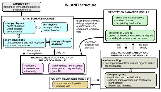
Figure 1.
Schematic of Integrated Model of Land Surface Processes (INLAND). Source: adapted from [17,29].
In the INLAND, a sub-model of conductance-photosynthesis based on photosynthesis models of C3 and C4 plants developed by [31,32] is responsible for estimating water and CO fluxes on an hourly scale. The differentiation in relation to the mode of carbon fixation and water loss by plants categorizes the plants in C3 and C4. In short, the process of fixing carbon dioxide in plants of type C3 is carried out through the Calvin Cycle by the enzyme RuBisCo, and forms a compound of 3-carbon (3PGA). Type C4 plants receive this name because they form, in the process of initial fixation of atmospheric CO in cells, an organic acid of 4-carbon molecules (oxaloacetate). This initial process is carried out by the enzyme PEP-carboxylase. Subsequently, the molecule is broken, releasing a CO molecule, which is fixed by the enzyme rubisco and transformed into sugars through the Calvin Cycle, similar to the photosynthesis of C3 plants [30,33].
2.1.1. NEE Modeling
The INLAND estimates the net ecosystem exchange of CO (NEE) from the difference between heterotrophic respiration () and net primary ecosystem production (NPP).
Negative values of the NEE indicate that an ecosystem is assimilating carbon while positive values indicate the emission of carbon. Heterotrophic respiration occurs based on the decomposition of leaves, roots, and stems by bacteria and is a function of the temperature and moisture of soil and carbon mass in the litter. In other words, denotes the emission of CO (stored in lignin and structural reservoirs) to the atmosphere during the decomposition of organic matter.
Based on equations proposed by [34,35,36], the model simulates carbon cycling occurring within the three reservoirs mentioned above (leaves, roots, and stems). To simulate these dynamics, it is necessary to introduce parameters associated with the carbon fraction of the litter layer stored in leaves (), roots (), and branches and stems () to the fraction stored in the soil (referring to humus physically or chemically protected, , and unprotected, , from decomposition), the decay rate of carbon reservoirs () and the leaf biomass turnover time constant (, in years).
The net primary productivity (NPP) of each functional plant type is calculated as a function of the gross photosynthesis rate, (mol CO m s), and from the respiration rate of the leaves, (mol CO m s), of fine roots, (mol CO m s) and of stems, (mol CO m s) [29]
where is a factor that attenuates NPP due to a carbon fraction lost as a result of plant development (i.e., the cost of building new tissues).
The respiration rates of fine roots and stems are given by
where and are carbon contained in woody and the fine roots, respectively, and are woody and fine root respiration coefficients (Kg y), and is the sapwood fraction of the stem biomass. The and functions are the Arrenhius [37] temperature functions for stems and soil defined respectively as
where is the stress coefficient for the biomass of stems, is the stress coefficient for biomass in the soil, and are the average temperatures of the upper canopy and root zone (K), respectively.
is estimated from the minimum value found between two potential rates of assimilation (, limiting the efficiency of the enzymatic system—Rubisco-limiting, and , limiting the amount of PAR captured by the leaf-light-limiting) according to the following equations:
where is the intrinsic quantum efficiency of the CO absorption of C3 plants (mol CO mol fotons), is the density flux of absorbed photosynthetically active radiation (mol fotons m s), is the concentration of CO in the intercellular spaces of leaves (mol mol), = [O]/2 is the compensation point for gross photosynthesis (mol mol), O is the atmospheric oxygen concentration, = [CO]/O is the ratio of kinetic parameters, where is the maximum Rubisco carboxylation capacity level (mol CO m s), and are the Michaelis–Mentem constants (mol mol) used to fix CO and to inhibit oxygenation, respectively.
The physiological limiting of assimilation (Rubisco-limiting), , is essentially controlled by the biochemical processing capacity of a leaf represented in the model by parameter . It is calculated from the product of the parameter of the maximum velocity of carboxylation of the Rubisco enzyme, , the temperature stress function, , and the soil moisture stress function, :
The temperature stress function is given by
where is the temperature stress coefficient of and where is the leaf temperature of the upper canopy (K).
The soil water stress function is expressed as
where is the parameter for soil moisture stress and is water available in the soil.
Vegetation temperature () is defined from the temperatures of leaves, stems, and both components (, , and , respectively) and from respective fractions per unit area (, , and ) according to the following equation
In the INLAND model, the connection between submodels of stomatal conductance and photosynthesis is given through leaf CO fluxes, which are considered to involve a one-dimensional diffusion process:
where is the CO concentration measured on the leaf boundary layer (mol mol), is the net assimilation photosynthesis rate (mol CO m s), where is the molar fraction of CO in the atmosphere (mol mol) and where is the boundary layer conductance of CO (mol CO m s).
The canopy stomatal conductance (mol CO m s) is written as
where m is the empirical coefficient of stomatal conductance, where b is the minimum stomatal conductance value (approximately 0.1 for C3 plants and 0.04 for C4 plants), and where is the relative humidity measured at the leaf surface.
Finally, is calculated as
The leaf respiration rate, , is calculated as the product between the leaf respiration coefficient of the Rubisco enzyme () and :
2.1.2. Modeling Soil Water Movement
The soil physics module simulates processes involved in soil water movement. Richards equations are used to simulate temporal variations in soil moisture determined as a function of soil hydraulic conductivity, the soil water retention curve and soil water uptake by roots. Vertical soil water movement through interlayers (m s m) is calculated on the basis of Darcy’s law [38,39]
where is hydraulic conductivity (m s), is volumetric water content (v v), and is the pressure head (m).
The INLAND model uses Campbell’s empirical formulations [39] to determine the soil moisture retention curve and soil hydraulic conductivity (relative to moisture):
where is air entry water potential (m), is the saturated hydraulic conductivity of soil (m s), and W is soil moisture calculated from ratio , where is saturated soil water content (or porosity). Exponent is an empirical parameter (Campbell’s parameter) related to the distribution of soil pore size. Variations in temperature, humidity, and water content levels in the soil are simulated with each time step for six layers of soil.
Vegetation cover represented in the INLAND varies according to the Plant Functional Type (PFT) involved. By default, 12 PFTs are represented in the model and each PFT is described according to its structural characteristics (leaf area index, vegetation layers—lower and upper canopy, and biomass) [17,29].
The vertical distribution of the root system follows the formulation proposed by [40]
where is the root fraction (ranging from 0 to 1) between soil depth d (cm) and total soil depth (cm). The root distribution parameter varies according to the type of plant concerned and according to different soil characteristics differentiated for the lower () and upper () canopies.
2.1.3. Distribution of Surface Energy
Net radiation and turbulent fluxes of sensible heat and water vapor determine changes in temperature and surface moisture levels. Solar and infrared radiation balances between the land surface, atmosphere, and vegetation canopy are simulated using the two-stream approach [41,42]. The approximation separately considers direct and diffuse radiation emitted within two wavelengths bands, visible (0.4–0.7 m), and infrared (0.7–4.0 m), which involve reflectance (, ) and transmittance parameters (, ) of the upper and lower layers of the canopy. Infrared radiation is simulated such that each vegetation layer is considered a semi-transparent plane [29]. Canopy emissivity is calculated as a function of the Leaf Area Index (LAI) and average diffuse optical depth coefficient () through an exponential relation.
Additionally, in calculating the radiative surface balance, fractions of direct and diffuse radiation that are directly scattered into the atmosphere are taken into account. For this, the model considers the canopy geometry through the orientation parameters of leaves of the upper () and lower () canopy.
Vegetation is dynamically represented by LAI estimates and by the amount of carbon assimilated by leaves for each PFT. Thus, plant growth or mortality is simulated in association with climatic conditions and is modeled by LAI and biomass variations for each PFT. The parameter indicates the potential LAI that contributes to plant carbon exchange, estimated by the product between and (specific leaf area (m Kg).
After estimating the surface net radiation (), the INLAND model partitions available energy into latent (), sensible (H), and soil (G) heat fluxes, using the relation:
H is calculated using the temperature difference of the air and upper canopy () and inversely proportional to aerodynamic resistance ()
where and are the air density and specific heat of air at constant pressure, respectively. Index u corresponds to the properties of the upper canopy. is dependent on properties of the land surface and on the logarithmic profile of wind
where is reference height, d is displacement of zero plane, is roughness length, is wind speed in reference height, and k is von Karman constant.
Similarly, is calculated as the sum of three water vapor fluxes
where is evaporation of water intercepted by canopies (leaves and stems), is canopy transpiration of canopy, and is evaporation from soil surface.
where () is fraction of leaves (stems) wetted by intercepted water, () is the air moisture deficit ( () is specific humidity of air at upper layer (reference height above upper layer), is stem area index, and is stomatal resistance, calculated from
where bulk canopy resistance coefficient and is wind speed at upper layer.
Stomatal resistance denotes resistance imposed by vegetation on the evapotranspiration process. It is basically dependent on the vegetation architecture and wind speed, from which the parameter (zero-plane displacement height coefficient d) is calibrated.
The heat flux of soil is calculated using the following equation
where is the balance between radiation absorbed by the soil and lost through turbulent fluxes, is precipitation intercepted by the soil, is the specific heat of the liquid water, is the surface flow, where is the difference between the temperature of rainfall and soil and where is the difference between the water freezing temperature and soil temperature.
2.2. Experimental Site
Atmospheric data and surface fluxes were obtained from January 2014 to December 2018 by a flux tower installed in the experimental area located in a natural vegetation (native fields) characteristic of the Pampa biome, near the city of Santa Maria, Rio Grande do Sul state, Brazil (lat −29.72; lon −53.77; alt 88 m elevation) (Figure 2). The experimental area is used for beef cattle, with the composition of the vegetation uniformly distributed in the area, predominant by Andropogon lateralis, Axonopus affinis, Paspalum notatum, and Aristida laevis [43,44]. The soil type is Planassolo Háplico Eutrofico [45], characterized with high fertility and high water retention. The soil physical proprieties are described in [46].
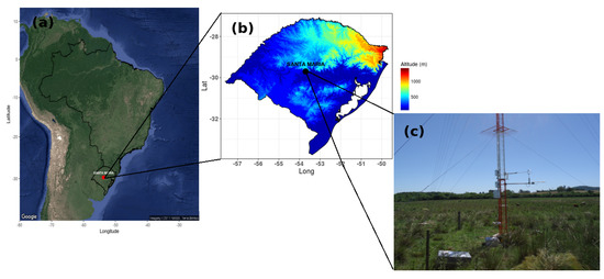
Figure 2.
(a) Location of the experimental site in South America and (b) in the state of Rio Grande do Sul (the color scale denotes the elevation of terrain at a resolution of 900 m) and (c) image of the micrometeorological tower.
The climate of the region is subtropical humid, belongs to the Cfa group in Köppen classification [47], with precipitation evenly distributed throughout the year. The climatic annual cumulative rainfall level () is 1545 mm while the average monthly climatological temperature () is approximately 20 C. These climatic values were obtained from the collected data between 1961 and 2013 by the Conventional Meteorological Station (OMM: 83936) located approximately 3.8 km away from the experimental site.
2.2.1. Meteorological and Flux Data
Atmospheric measurements were collected by the flux tower using the 3D sonic anemometer (Wind Master Pro; Gill Instruments, Hampshire, UK) measuring wind and air temperature components, a gas analyzer (LI7500, LI-COR Inc., Lincoln, NE, USA) measuring the HO and CO concentration sampled at a 10 Hz. Additionally measured were air temperature and relative humidity with a thermo-hygrometer (HMP155, Vaisala, Finland) and precipitation with a rainfall sensor (TR525USW, Texas Electronics, TX, USA), and net radiation and short-wave incident radiation sensors (CNR4, Kipp & Zonen, Delft, The Netherlands). All measurements occurred at 3 m height. Soil heat flux was measured with soil heat plates (HFP01, Hukseflux Thermal Sensors B.V., Delft, The Netherlands) placed at 0.10 m depth and soil water content was measured using water content reflectometers (CS 616, Campbell Scientific Inc., Logan, UT, USA) at a depth of 0.10 m.
The forcing data were gap filled. Missing data occurred due to power outages and equipment malfunctions. Missing , , , , and were filled directly with data collected from the Automatic Weather Station—AWS (OMM: 86977) located approximately 3.8 km away from the experimental site. After this procedure, gaps remain in (0.05%) and (0.03%) data were filled through the application of the inverse distance weighted interpolation method [48] using data of neighboring AWSs positioned within a 200 km radius of Santa Maria. For incident long wave radiation gaps (7.32%), we follow Aimi et al. (2020) (manuscript in preparation).
The turbulent fluxes, latent () and sensible (H) heat fluxes, and CO flux were estimated by Eddy Covariance (EC) method [49] using EddyPro software version 6.1 (Li-Cor, Lincoln, NE, USA), with the same configurations as [46] (30-min average from high frequency data −10 Hz). No gap filling was used in turbulent fluxes data.
The energy balance (EB) closure () was used to filter the fluxes. The energy balance ratio () given by the ratio between the cumulative sum of available energy () and turbulent fluxes ():
Fluxes of lower (upper) values of the 1% (99%) percentile for the given time step were excluded from the analyses. Flux data with “poor” BE closure values [25,50,51] were removed. In this case, the inequality written is as
where , must be satisfied. Thus, we only consider values with daily energy component sums measured by the EC method of within 80% of the energy balance measured from radiative instruments and from the heat flux of the soil. The daily averages of turbulent fluxes were calculated considering the days on which at least 19 hourly measurements were recorded (at least 80% of the measures).
2.2.2. Model Initialization: Soil Moisture Spin-up
Meteorological datasets collected in Santa Maria experimental site (as described in Section 2.2.1) for 1 January 2014 to 31 December 2018 were used as input data to the model: , , , , and .
To initialize the model (spin-up) forced by hourly average data, the difference in total column soil moisture from one year to another was set as less than 0.1% [14,52]. The results show a spin-up time of approximately six years consistent with the results of [53]. Thus, in this work, the model simulation period was set to eleven years, and only the last five years were analyzed in relation to the experimental data.
2.3. Calibration: Hierarchical and Multi-Objective Approach
In this study, we calibrated the surface fluxes (, H, , and ) to solve a multi-criteria optimization problem [10,12,13]. INLAND parameters were automatically calibrated using the genetically adaptive multi-objective calibration method (AMALGAM) [11], which allows finding a set of parameters that defines the “Pareto-optimal” curve corresponding to a vector of multiple objective functions. The AMALGAM combines several genetic algorithms that adapt to the problem of multiple optimization to simultaneously optimize more than one objective function.
Mathematically, the problem involves minimizing m () objective functions with d parameters
where denotes the vector with the set of parameters (decision vector) and where F is the objective space. The search space of values of x can be quite large, but it must be delimited in . Thus, rather than finding a single optimal solution, we find a Pareto-optimal set of solutions. The objective functions used in the calibration included the root mean square error () and the amplitude of the daily average cycle error () (Table 1). However, AMALGAM allows the use of only one metric if calibration involves more than one variable (output of model). On the other hand, if we use more than one metric, we must choose only one variable.

Table 1.
Metrics used to evaluate the performance of the calibration and its mathematical formulations. n is the length of the series, S and O correspond to the simulated and observed data, respectively, denotes the average daily cycle amplitude, and is the mean of S.
The different hierarquical framework of the processes represented in INLAND are used to define the hierarchical levels of calibration and model output: level 1—radiation fluxes (for parameters used in reflected solar radiation—), and level 2—turbulent fluxes (for parameters used in , , and H). The metrics used to calibrated were and . On the other hand, the metric used for , H, and was for a better representation of these fluxes in average terms. The parameters calibrated in this work are presented in Table 2 following the studies developed by [9,13,25]
Table 2.
Structure of the multi-objective calibration: hierarchical levels, variables, metrics, parameters, default values, ranges, and calibrated values used in the INLAND model. and represent the visible and near infrared bands, respectively.
2.4. Simulations Design And Analyses
The model was calibrated using data collected between 1 January 2014, and 31 December 2017 on an hourly time scale. The model was run using scripts developed through R software [54] such that the calibration algorithm automatically interacted with the surface model, testing each parameter within respective ranges of variation (Table 2). The selection of the intervals was based on previous studies [13,14,25] and also on the calibration design, since eventually the calibrated parameters reached the limits of the intervals, indicating the increase of the same.
For all simulations the model was run in offline mode using a single-point version with static vegetation (FTP = 12 corresponding type C3 grasses) and the LAI = 2.25 m m (annual mean from 2014 to 2015 of data obtained by MOD15A2 product of MODIS freely available at https://modis.ornl.gov/). Runs for model validation were performed with hourly data for January 1 to December 31, 2018 using the same calibration settings. The six thicknesses of the soil layers were defined in meters as 0.05, 0.10, 0.15, 0.30, 0.40, and 0.50, covering a depth of 1.5 m.
R software scripts were developed to analyze results obtained from the different calibrations. This analysis was performed based on metrics described in Table 1. The and best values should be near one and for , , , near zero. To evaluate the calibration performance, we analyzed the model outputs against the experimental data of , , , , H, , and . The values of prognostic variables simulated with INLAND using default parameters (referenced as def) and parameters calibrated showed in Table 2 (referenced as clb) were compared with observed data using the statistic described in Table 1.
3. Results and Discussion
3.1. Weather Conditions
Monthly averages of accumulated rainfall collected in the 2014 to 2018 years were found to be significantly higher than climatological (Pclim) values (Figure 3). Accumulated annual precipitation levels registered for 2014, 2015, and 2017 are 2033 mm, 1938 mm, and 1821 mm, respectively, approximately 32%, 26%, and 18% higher than climatology values. On the other hand, the years 2016 and 2018 presented annual accumulated very close to climatology (differences of −6% and −7%). Monthly, the winter months presented greater variability in precipitation and air temperature. Average monthly air temperatures observed for the first six months of both years (2014 and 2015) were consistently lower than those recorded climatologically. On the other hand, for the months of July, September, and October 2014, the average monthly temperature was slightly higher than the climatology value. The second half of 2015 also presented temperatures falling below climatological values except for the month of August, for which values surpassed the climatological average at approximately 4 C. Average annual temperatures for 2014 (19.7 C), 2015 (19.6 C), 2016 (19 C), 2018 (19.6 C), and the climatological average (20.2 C) were found to be very similar. The 2017 year was the only year with a positive difference from , recording an average annual temperature of 20.3 C.
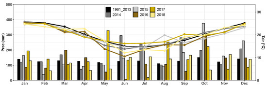
Figure 3.
Cumulative monthly rainfall (mm) and average monthly temperature (C) observed at the experimental site (2014 to 2018) and at the Conventional Weather Station (CWS) of National Institute of Meteorology (INMET) from 1961 to 2013.
3.2. Calibration
Table 2 shows the values of the calibrated parameters for the Pampa biome using INLAND model with AMALGAM calibration method. The parameters are associated with their respective hierarchical levels of calibration. The sensitive difference between the default values of the model for this vegetation type and the calibrated values can be clearly observed. This fact further highlights the importance of calibration, since, although the model individualizes the representation of different vegetation types, local environmental conditions significantly alter their input parameters, causing errors in the simulations.
The first calibration level calibrates parameters that influence the determination of the surface net radiation. The daily average of solar radiation reflected by the surface presents good agreement with the observed data after calibration, the RMSE and PBIAS decrease significantly (Figure 4 and Table 3). The seasonality and the daily cycle of the are well represented.
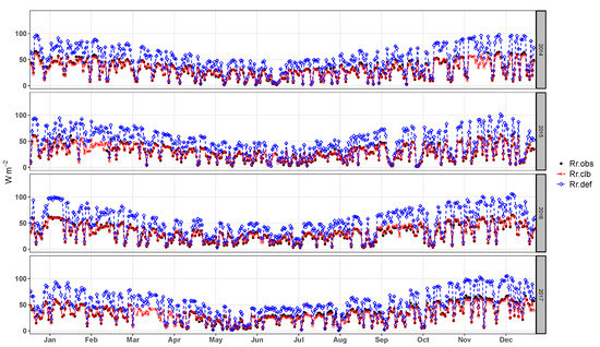
Figure 4.
Daily average of the solar radiation reflected by the surface observed (), simulated by the model before calibration () and simulated after the calibration ().
Table 3.
Daily average statistics of the simulated values (calibrated and default ) against data observed from the Santa Maria experimental site from 2014 to 2017, for net radiation (Rn), solar radiation reflected by the surface (Rr), latent heat flux (LE), sensible heat flux (H), and net ecosystem exchange of CO (NEE).
The model satisfactorily reproduced the average diurnal cycle of the (Figure 5), which is of critical importance to the correct representation of latent, sensible, and soil heat flux, as the balance of radiation determines the amount of energy available for such fluxes. In addition, the coefficient of determination close to one (Table 3) for the calibrated and observed daily data reinforces that calibration significantly improved the simulation of this variable.
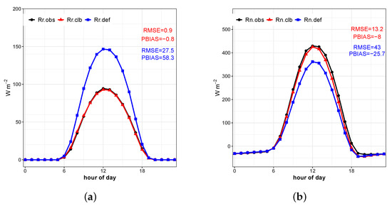
Figure 5.
(a) Average diurnal cycle of solar radiation reflected by the surface observed (), simulated by the model before calibration (), and simulated after the calibration (); (b) same for .
Analyzing monthly means of surface albedo (ratio between the solar radiation reflected by the surface and incoming shortwave radiation in the surface), we can observe that using default parameters, the mean albedo were 0.27 for 2014 and 2015, and were 0.28 for 2016 and 2017, while observed data were 0.18 for 2014 and 2017, and were 0.17 for 2015 and 2016. That is an approximate difference of 0.1 for the entire period. After calibration the simulated value was 0.18 (Figure 6) for the four years. It is important to note that there is almost no seasonal variation of this variable.
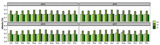
Figure 6.
Average monthly albedo observed (), simulated by the model before calibration () and simulated after calibration ().
The second calibration level corresponds to turbulent fluxes. The calibrated model improved the representation (Figure 7). This improvement is evident for the months of January to March and of October to December, periods in which values are higher than those for the rest of the year. The seasonality of accompanies the seasonality of the , showing that this component strongly controls evaporation and transpiration processes of the Pampa biome.
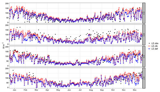
Figure 7.
Daily average latent heat flux observed (), simulated by the model before calibration (), and simulated after the calibration ().
The average diurnal cycle and scatter plot of for 2014 to 2017 shown in Figure 8 shows that the calibrated simulation makes significant improvements relative to the default simulation, especially for the daytime period. The difference between the peak and of approximately 40 W m found stands out while the difference found between and does not exceed a value of 10 W m. In addition, a clear trend in the model can be observed in its overestimation of values for the daytime values. We also highlight the good fit of the linear regression line between calibrated and observed hourly values (m = 0.94, b = 8.35, and R2 = 0.77), which is substantially better than values shown in the literature [13,25].
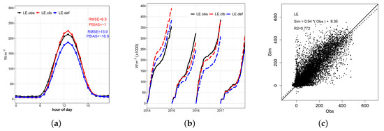
Figure 8.
(a) Average diurnal cycle of latent heat flux observed (), simulated by the model before calibration (), and simulated after the calibration (); (b) daily cumulative sum by year; (c) scatter plot of hourly observed and simulated by the calibrated model.
Daily mean values (Figure 9) and average diurnal cycles simulated (Figure 10) for sensible heat flux, simulated with the calibrated parameters show significant improvements relative to the default simulation. However, unlike values for , the model did not reproduce the annual seasonality of observed H for the Pampa biome.
Figure 9.
Daily average of sensible heat flux observed (), simulated by the model before calibration (), and simulated after the calibration ().
Figure 10.
(a) Average diurnal cycle of sensible heat flux observed (), simulated by the model before calibration (), and simulated after the calibration (); (b) daily H cumulative sum by year; (c) scatter plot of hourly H observed and simulated by the calibrated model.
Different patterns between the simulated diurnal and nocturnal periods in relation to those observed are found. Systematic underestimations between 6 and 12 a.m. and overestimations between 1 and 6 p.m. (Figure 10). The scatter plot shows good adjustment in relation to the hourly observed data (angular coefficient 0.83, linear coefficient 12.3 and 0.78). It is also possible to observe a slight lag in simulated values covering approximately one hour at the upper peak of H and underestimations at this point of approximately 5 W m and 40 W m for and , respectively.
Good fit of the mean daily values by year and average diurnal cycle of the for daytime periods (diurnal and nocturnal) can be observed in Figure 11 and Figure 12a, respectively. Values of for the daytime period present great discrepancies in relation to the observed data. Coefficients of the regression line for hourly values present values of m = 0.75 and b = −1, which are similar to the values found by [13].
Figure 11.
Daily average of NEE observed (), simulated by the model before calibration (), and simulated after the calibration ().
Figure 12.
(a) Average diurnal cycle of the net ecosystem exchange of CO observed (), simulated by the model before calibration (), and simulated after the calibration (); (b) daily cumulative sum by year; (c) scatter plot of hourly observed and simulated by the calibrated model.
The daily cumulative sums by year of , H, and (Figure 8b, Figure 10b and Figure 12b) show that the calibration of the model substantially improved the representation of these variables. Especially for simulated LE in 2016 and 2017, the accumulated differences did not exceed 10%. On the other hand, despite the noticeable improvement in the accumulated annual NEE computation compared to the default simulation, it is noted that the model still greatly overestimates the carbon assimilation in the Pampa.
Figure 13 shows the cumulative distribution function (CDF) of daily differences observed between the simulations of the default and calibrated parameters in relation to observed values of variables , , H and . This result reinforces the improvement that the model made after calibration. In particular, underestimates of 8 mol CO ms or more accounted for approximately 35% of the and for 0% of the . That is, the calibration of the model parameters related to the calculation of CO flux (mainly , , , and m) was able to substantially reduce estimation errors.
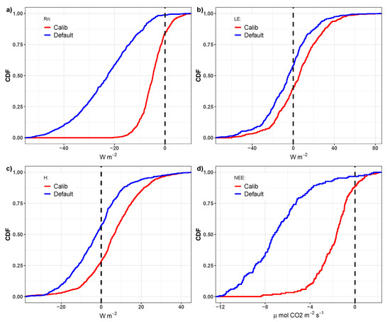
Figure 13.
Cumulative distribution function (CDF) of daily differences between the simulations using the default and calibrated parameters in relation to the observed values of the variables (a), (b), H (c), and (d).
3.3. Discussion
Although C3 and C4 type plants co-exist in the Pampa biome, there is a predominance of C3 metabolism plants as described by [27]. Tests were performed using FTP = 11 (C4 grasses) and FTP = 12 (C3 grasses); however, better results of statistical index were obtained for the FTP = 12, and the calibration was performed using this FTP. In addition, at the experimental site where the data were collected, there are herbivorous animals, especially beef cattle, managed under the grazing system. The presence of these animals is a common feature of the Pampa biome [55]. The model does not take into account the biomass extracted by the animals, however we understand that the calibration makes this representation. Inserting the biomass removal by herbivores in the model would be a structural change that is being implemented by BESM. As the animal load in the Pampa biome is, on average, uniform, this calibration can be used for the entire area covered by the biome.
Regarding turbulent flux parameters (level 2), parameter (the maximum velocity of carboxylation) stands out, representing a measure of the process through which enzyme Rubisco produces carbon compounds that become sugars and starches. This parameter has a direct impact on gross primary productivity (GPP) levels and consequently on and can be considered representative of large regions provided that they include plant cover with similar plant species [9].
For all simulated variables, a significant improvement in results occurs after calibration. , , and presented the most significant improvements, especially in relation to daily averages. For the nocturnal period, practically no improvement in latent heat flux was seen. On the other hand, the diurnal representation of this variable improved remarkably.
Decoupling between the simulated and the data observed for mid-April 2014, 2016, and 2017 (Figure 8b) was also reported by [25], who simulated the Brazilian Caatinga region. [25] describes limitations of the IBIS model in simulating latent heat fluxes when abrupt changes occur in the precipitation regime, especially because the model fails to capture large variations in the LAI for these periods. In fact, the LAI is a determining factor along with the radiative component that shapes evapotranspiration. However, unlike Caatinga, in which vegetation is predominantly xeromorphic, vegetation that predominates in the Pampa biome (Campos) is characterized by high levels of photosynthetic activity throughout the year and by an almost constant LAI.
Southern Brazil does not experience dry and wet seasons as in semi-arid regions of Brazil, but rather two periods of the year are defined primarily by temperature variations: hot summer and cold winter seasons Figure 3. Both seasons are characterized by high precipitation volumes that are well distributed, and consequently soil water content levels remain high almost year-round ([46,56]). Thus, among other factors, it can be said that the model failed to reproduce the reduction of the due to a decrease in photosynthetic activity associated with a reduction in surface temperature.
Solar radiation reflected by the surface also partly explains errors found in the simulation. is underestimated by 2 W m on average for almost every month of the year. Thus, for the model, with more energy available on the land surface, more energy is available for evapotranspiration, overestimating the observed value.
The largest discrepancies between the calibrated simulation and observed data were found in sensible heat flux levels with high bias and RMSE values. This can be explained by the consistently poor simulation of daytime fluxes. The H simulation errors found may have resulted for two main reasons. The first is related to errors of 10 to 30% found in estimates of the observed fluxes by the Eddy Covariance system. As the model is based on the principle of energy conservation, such uncertainties violate this principle. A similar result was found by [13], although it was observed that the model overestimated H for the nocturnal period and mainly due to overestimation.
The second reason is related to the poor representation of soil heat flux (G) by the model. In general, overestimation of daytime G (10 to 50 W m, not shown) occurs. Again, as the model seeks energy balance closure, it compensates for this surplus by understating H. The results of this study are similar to those reported in the literature [25,57,58,59]. Ref. [60] noted that not considering a residual layer on the land surface can result in such overestimation. In addition, the LSEM tends to overestimate G and mainly due to the low numerical resolution of soil temperatures close to the land surface, resulting in a delay in the representation of turbulent fluxes [56]. This is clear in the CMD representation of H (Figure 10a) and G (not shown). A decoupling of and curves is observed for the early hours of the morning. By the end of the afternoon, approximately after 5 p.m., the curves are similar again, precisely when differences with respect to G are smaller.
Figure 14 shows the hysteresis of latent heat flux and sensible heat flux and net ecosystem exchange patterns of CO against atmospheric variables air temperature (), the vapor pressure deficit () and global radiation (). Here, we clearly find the most pronounced errors for H. While follows intense hysteresis patterns with respect to and , H underestimates the observed flux lag although it do follow the roughly elliptical form of the curves. In relation to , we find an overestimation of the mismatch and a displacement (rotation) of hysteresis in relation to H. These results reinforce the model’s difficulty in simulating H, showing the better representation of parameterizations of this flux in relation to atmospheric forcing must be explored.
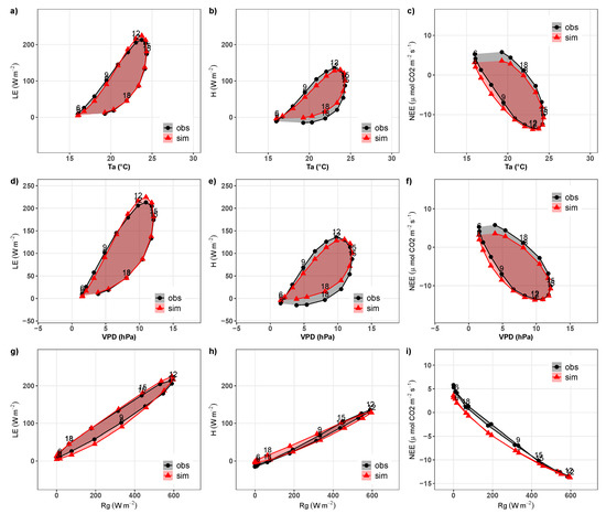
Figure 14.
Hysteresis loops relating: (a) latent heat flux () against air temperature (), (b) sensible heat flux (H) against , (c) net ecosystem exchange of CO () against , (d) against deficit of water vapor pressure (), (e) H against , (f) against , (g) against global radiation (), (h) H against , and (i) against . Graphs correspond to observed values () and simulated after calibration () to the experimental site located in Santa Maria, southern Brazil, from 2014 to 2017. Numbers represent the hours of the day.
Finally, the simulation of the net ecosystem exchange of CO with the calibrated INLAND very closely reflected observed values and mainly in relation to the CMD. For the nocturnal period, we observed a slight underestimation of (positive values); that is, the model is underestimating the ecosystem respiration. On the other hand, for the daytime period, the model overestimated (negative values), indicating that the model overestimates the photosynthesis in the ecosystem. Despite this, good agreement between and atmospheric forcing was found as illustrated by the strong representation of hysteresis in relation to , , and (Figure 14). Moreover, in natural pasture of the Pampa biome, the presence of cattle is common [26]. The presence of these animals can affect , especially by soil fertilization.
3.4. Validation and Annual Estimation
The INLAND model was validated from atmospheric forcing and turbulent flux data collected at the Santa Maria experimental site from 1 January to 31 December 2018. Figure 15 shows the daily time series of the net radiation, latent and sensible heat fluxes, and the net ecosystem exchange of CO. In this comparison, we had 212 daily measurements observed to , , H, and 110 to . In general, we find a good fit between the simulated and observed data, indicating that the multi-objective calibration generated positive model simulation results. and were slightly underestimated by the model (PBIAS −2.6 and −4, respectively) while H and were overestimated (PBIAS 24 and 20) while maintaining low values (similar to those found from the calibration). In average terms the calibration of model can successfully represent the observed patterns (RMSE 15, 15, and 14 W m for , , and H, respectively, and 1.7 mol CO ms for ), especially compared to the default simulation (RMSE 31, 22, and 14 W m for , , and H, respectively, and 6.4 mol CO ms for , respectively).
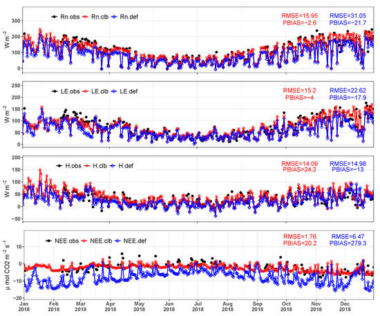
Figure 15.
Daily average net radiation (), latent heat flux (), sensible heat flux (H), and net ecosystem exchange of CO () observed () and simulated by the model before calibration () and after the calibration () to the validation period (January to December 2018). Daily average statistics are shown in the graphics area.
The good agreement of the simulations for the validation period is confirmed by the graphs of the average diurnal cycles of , , H, and (Figure 16). Although there are still small discrepancies in the nocturnal period of the variables H and , it is possible to observe that the calibration substantially improves all the fluxes analyzed, especially in relation to and for the whole day and H and for the diurnal period.
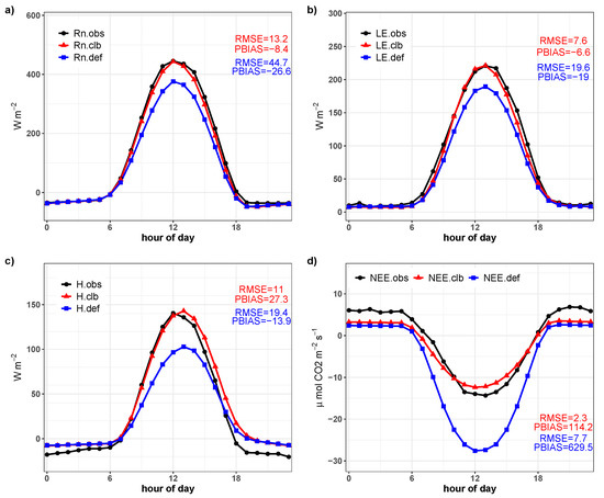
Figure 16.
Average diurnal cycle of observed (), simulated by the model before calibration (), and simulated after the calibration () from January to December, 2018. (a) Net radiation, [W m]; (b) latent heat flux, [W m]; (c) sensible heat flux, H [W m]; and (d) net ecosystem exchange of CO, [mol CO, ms]. Hourly statistics are shown in the graphics area.
Figure 17 shows scatter plots for , the and H fluxes and the value. The simulation of from the calibrated model shows excellent adjustment in relation to the observed data. The angular coefficient of close to 1 (0.97) and the linear coefficient of close to zero (−3.5) show that the simulation closely reflects the observed values. Values of the coefficients are similar to those found by [13,25], who used similar models to that used in this work. and H simulated after calibration also exhibit good adjustment in relation to the observed data. Both fluxes present high coefficients of determination (0.89 for and H). is also well adjusted with values of coefficients of the regression line (angular 0.61 and linear −2.19) considered satisfactory.
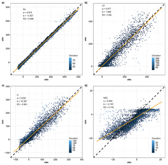
Figure 17.
Scatterplots of the simulated hourly values against data observed from the Santa Maria experimental site from January to December, 2018. (a) Net radiation, [W m]; (b) latent heat flux, [W m]; (c) sensible heat flux, H [W m]; and (d) net ecosystem exchange of CO, [mol CO ms].
Overestimates of latent sensible heat flux are predominant in the validation period with 77% of differences between simulated and observed values greater than zero. However, the daily estimates of were well divided throughout the year, with 52% of the days with overestimates and 48% with underestimates. Added to this, the average annual estimate of simulated was approximately 905 mm year, values very close to those found in the literature for the Pampa biome (898 mm year, [46]).
4. Conclusions
In this work, we improve the representation of surface processes that occur in the Pampa biome through the use of a hierarchical and multi-objective calibration applied to the INLAND model. The AMALGAM algorithm enabled the calibration of the model based on multiple objective functions (two metrics and four model outputs) used in a hierarchical time sequence that follows the biogeophysical and biogeochemical processes of natural systems. The calibration results were evaluated based on data collected from an experimental site with vegetation representative of the Pampa biome.
In general, the simulations satisfactorily represented energy and mass changes occurring within the examined ecosystem. For the calibration period, the simulation of net radiation generated the best results. After calibration, the average diurnal cycle and daily mean of generated satisfactory statistics (e.g., there was a reduction of roughly 65% in mean absolute error). For daily averages, latent heat flux was slightly overestimated but with a magnitude of error comparable to related works in the literature. Values such as the RMSE were decreased by approximately 10% in relation to those of the default simulation. On the other hand, the sensible heat flux was systematically overestimated by the model. This characteristic of the model, which has also been reported in other works, may be related to deficiencies of physical parameterizations used by the model to represent heat transfer between vegetation and the atmosphere.
Slight underestimates of the net CO exchange of the ecosystem were observed and mainly in relation to annual accumulation. Despite this, the INLAND representation of was substantially improved after calibration, reducing the absolute mean error of daily values by more than 69%. Nocturnal assimilation was systematically underestimated while daytime values and mainly for between 9 a.m. and 3 p.m. were overestimated by the model. This problem may be associated with an underestimation of diurnal respiration rates, whose origins may be associated with errors of coefficients related to soil respiration or soil carbon content. To investigate this problem, it is necessary to collected field measurements that allow for more accurate comparisons. This is an important theme to be explored in future work.
Surface cover plays a key role in physical and ecological processes that occur throughout the atmospheric boundary layer. Especially for surfaces covered by native vegetation, understanding interactions between the land surface and atmosphere and the role of vegetation in physical and ecological processes that govern biosphere behavior has expanded significantly in recent years. As a result, LSEMs are increasingly being designed to represent more complex processes at different time scales. Of course, in increasing the variety and complexity of representations of natural processes using surface models we must examine more processes in a more complex manner. Therefore, it is necessary to apply robust methodologies to calibrate and validate such models using experimental data.
This work is the first to accomplish the multi-objective calibration of an LSEM for a site with vegetation representative of the Pampa biome. It should be noted that studies considering flux data for multiple experimental sites with similar vegetation are necessary to eliminate effects of differences in ecosystem composition. In addition, as the biome has the presence of C3 and C4 plants and has the constant presence of cattle, a new PFT could be included in the model by modeling these biome features. However, the parameters calibrated in this manuscript allow to INLAND model represent more realistically the surface process in the Pampa biome considering the climatic variability throughout the years. This ensures, within its limitations, the safe use of the model for studies of how vegetation can affect local and regional climate, especially when coupled with Atmospheric General Circulation Models. In addition, the calibration and validation performed in this work provide a precise set of parameters for future applications of the INLAND to studies on the impacts of changes in land use and land cover on the Pampa biome.
Author Contributions
G.G. and R.H.V. were responsible for research design, analysis and interpreting the results, and land-surface model simulations. D.R.R. and G.A.D. were resposible for conceptualization and administration of the project, and data curation. D.L.H. was responsible for the funding acquisition. G.G., D.R.R., D.L.H. and L.G.G.d.G. helped carry out the methodology, analysis and writing of the manuscript, and writing-review and editing. R.A.G. helped processed data and data curation. All authors have read and agreed to the published version of the manuscript.
Funding
This study was financed in part by Coordination for the Improvement of Higher Education Personal (CAPES-Brazil).
Acknowledgments
The authors acknowledge the National Council for Scientific and Technological Development (CNPq—Brazil), the Foundation for Research of Rio Grande do Sul State (FAPERGS) for their financial support and the Coordination for the Improvement of Higher Education Personnel (CAPES—Brazil), for partially funding this work through the project CAPES/Modelagem 88881.148662/2017-01. We gratefully thank to the Federal University of Pampa (UNIPAMPA), the staff of the Micrometeorology Lab of the Federal University of Santa Maria (UFSM) and the Research Group on Atmosphere-Biosphere Interaction of the Federal University of Viçosa (UFV) for technical and structural support. The authors would also like to thank the anonymous reviewers for significantly improving the clarity of our manuscript and helpful comments.
Conflicts of Interest
The authors declare no conflict of interest.
References
- Bonan, G.B. Forests and Climate Change: Forcings, Feedbacks, and the Climate Benefits of Forests. Science 2008, 320, 1444–1449. [Google Scholar] [CrossRef]
- Pitman, A.J. The evolution of, and revolution in, land surface schemes designed for climate models. Int. J. Climatol. 2003, 23, 479–510. [Google Scholar] [CrossRef]
- VanLoocke, A.; Twine, T.E.; Zeri, M.; Bernacchi, C.J. A regional comparison of water use efficiency for miscanthus, switchgrass and maize. Agric. For. Meteorol. 2012, 164, 82–95. [Google Scholar] [CrossRef]
- Zhang, K.; Castanho, A.D.d.A.; Galbraith, D.R.; Moghim, S.; Levine, N.M.; Bras, R.L.; Coe, M.T.; Costa, M.H.; Malhi, Y.; Longo, M.; et al. The fate of Amazonian ecosystems over the coming century arising from changes in climate, atmospheric CO2, and land use. Glob. Chang. Biol. 2015, 21, 2569–2587. [Google Scholar] [CrossRef]
- Chen, M.; Willgoose, G.R.; Saco, P.M. Evaluation of the hydrology of the IBIS land surface model in a semi-arid catchment. Hydrol. Process. 2015, 29, 653–670. [Google Scholar] [CrossRef]
- Gupta, H.V.; Bastidas, L.A.; Sorooshian, S.; Shuttleworth, W.J.; Yang, Z.L. Parameter estimation of a land surface scheme using multicriteria methods. J. Geophys. Res. Atmos. 1999, 104, 19491–19503. [Google Scholar] [CrossRef]
- Groenendijk, M.; Dolman, A.; van der Molen, M.; Leuning, R.; Arneth, A.; Delpierre, N.; Gash, J.; Lindroth, A.; Richardson, A.; Verbeeck, H.; et al. Assessing parameter variability in a photosynthesis model within and between plant functional types using global Fluxnet eddy covariance data. Agric. For. Meteorol. 2011, 151, 22–38. [Google Scholar] [CrossRef]
- da Rocha, H.R.; Nobre, C.A.; Bonatti, J.P.; Wright, I.R.; Sellers, P.J. A vegetation-atmosphere interaction study for Amazonia deforestation using field data and a ‘single column’ model. Q. J. R. Meteorol. Soc. 1996, 122, 567–594. [Google Scholar]
- Fischer, G.R.; Costa, M.H.; Murta, F.Z.; Malhado, A.C.; Aguiar, L.J.; Ladle, R.J. Multi-site land surface model optimization: An exploration of objective functions. Agric. For. Meteorol. 2013, 182, 168–176. [Google Scholar] [CrossRef]
- Boyle, D.P.; Gupta, H.V.; Sorooshian, S. Toward improved calibration of hydrologic models: Combining the strengths of manual and automatic methods. Water Resour. Res. 2000, 36, 3663–3674. [Google Scholar] [CrossRef]
- Vrugt, J.A.; Robinson, B.A. Improved evolutionary optimization from genetically adaptive multimethod search. Proc. Natl. Acad. Sci. USA 2007, 104, 708–711. [Google Scholar] [CrossRef]
- Xue, L.; Pan, Z. Ensemble calibration and sensitivity study of a surface CO2 flux scheme using an optimization algorithm. J. Geophys. Res. Atmos. 2008, 113. [Google Scholar] [CrossRef]
- Varejão, C.G.; Costa, M.H.; Camargo, C.C.S. A multi-objective hierarchical calibration procedure for land surface/ecosystem models. Inverse Probl. Sci. Eng. 2013, 21, 357–386. [Google Scholar] [CrossRef]
- Rosolem, R.; Gupta, H.V.; Shuttleworth, W.J.; de Gonçalves, L.G.G.; Zeng, X. Towards a comprehensive approach to parameter estimation in land surface parameterization schemes. Hydrol. Process. 2012, 27, 2075–2097. [Google Scholar] [CrossRef]
- Wöhling, T.; Samaniego, L.; Kumar, R. Evaluating multiple performance criteria to calibrate the distributed hydrological model of the upper Neckar catchment. Environ. Earth Sci. 2013, 69, 453–468. [Google Scholar] [CrossRef]
- Shafii, M.; Tolson, B.A. Optimizing hydrological consistency by incorporating hydrological signatures into model calibration objectives. Water Resour. Res. 2015, 51, 3796–3814. [Google Scholar] [CrossRef]
- Foley, J.A.; Prentice, I.C.; Ramankutty, N.; Levis, S.; Pollard, D.; Sitch, S.; Haxeltine, A. An integrated biosphere model of land surface processes, terrestrial carbon balance, and vegetation dynamics. Glob. Biogeochem. Cycles 1996, 10, 603–628. [Google Scholar] [CrossRef]
- Costa, M.H.; Pires, G.F. Effects of Amazon and Central Brazil deforestation scenarios on the duration of the dry season in the arc of deforestation. Int. J. Climatol. 2010, 30, 1970–1979. [Google Scholar] [CrossRef]
- Castanho, A.D.A.; Coe, M.T.; Costa, M.H.; Malhi, Y.; Galbraith, D.; Quesada, C.A. Improving simulated Amazon forest biomass and productivity by including spatial variation in biophysical parameters. Biogeosciences 2013, 10, 2255–2272. [Google Scholar] [CrossRef]
- Castanho, A.D.A.; Galbraith, D.; Zhang, K.; Coe, M.T.; Costa, M.H.; Moorcroft, P. Changing Amazon biomass and the role of atmospheric CO2 concentration, climate, and land use. Glob. Biogeochem. Cycles 2016, 30, 18–39. [Google Scholar] [CrossRef]
- Pires, G.F.; Abrahão, G.M.; Brumatti, L.M.; Oliveira, L.J.; Costa, M.H.; Liddicoat, S.; Kato, E.; Ladle, R.J. Increased climate risk in Brazilian double cropping agriculture systems: Implications for land use in Northern Brazil. Agric. For. Meteorol. 2016, 228–229, 286–298. [Google Scholar] [CrossRef]
- Restrepo-Coupe, N.; Levine, N.M.; Christoffersen, B.O.; Albert, L.P.; Wu, J.; Costa, M.H.; Galbraith, D.; Imbuzeiro, H.; Martins, G.; da Araujo, A.C.; et al. Do dynamic global vegetation models capture the seasonality of carbon fluxes in the Amazon basin? A data-model intercomparison. Glob. Chang. Biol. 2017, 23, 191–208. [Google Scholar] [CrossRef]
- Dionizio, E.A.; Costa, M.H.; Castanho, A.D.D.A.; Pires, G.F.; Marimon, B.S.; Marimon-Junior, B.H.; Lenza, E.; Pimenta, F.M.; Yang, X.; Jain, A.K. Influence of climate variability, fire and phosphorus limitation on vegetation structure and dynamics of the Amazon-Cerrado border. Biogeosciences 2018, 15, 919–936. [Google Scholar] [CrossRef]
- Figueroa, S.N.; Bonatti, J.P.; Kubota, P.Y.; Grell, G.A.; Morrison, H.; Barros, S.R.M.; Fernandez, J.P.R.; Ramirez, E.; Siqueira, L.; Luzia, G.; et al. The Brazilian Global Atmospheric Model (BAM): Performance for Tropical Rainfall Forecasting and Sensitivity to Convective Scheme and Horizontal Resolution. Weather Forecast. 2016, 31, 1547–1572. [Google Scholar] [CrossRef]
- Cunha, A.P.M.A.; Alvalá, R.C.S.; Sampaio, G.; Shimizu, M.H.; Costa, M.H. Calibration and Validation of the Integrated Biosphere Simulator (IBIS) for a Brazilian Semiarid Region. J. Appl. Meteorol. Climatol. 2013, 52, 2753–2770. [Google Scholar] [CrossRef]
- Overbeck, G.E.; Müller, S.C.; Fidelis, A.; Pfadenhauer, J.; Pillar, V.D.; Blanco, C.C.; Boldrini, I.I.; Both, R.; Forneck, E.D. Brazil’s neglected biome: The South Brazilian Campos. Perspect. Plant Ecol. Evol. Syst. 2007, 9, 101–116. [Google Scholar] [CrossRef]
- Pillar, V.P.; Muller, S.C.; Castilhos, Z.M.S.; Jacques, A.V.A. Campos Sulinos-Conservação e uso Sustentável da Biodiversidade; MMA: Brasília, Brazil, 2009; p. 403. [Google Scholar]
- Boldrini, I.I.; Eggers, L. Vegetação campestre do sul do Brasil: Dinâmica de espécies a exclusão do gado. Acta Bot. Bras. 1996, 10, 37–50. [Google Scholar] [CrossRef]
- Kucharik, C.J.; Foley, J.A.; Delire, C.; Fisher, V.A.; Coe, M.T.; Lenters, J.D.; Young-Molling, C.; Ramankutty, N.; Norman, J.M.; Gower, S.T. Testing the performance of a dynamic global ecosystem model: Water balance, carbon balance, and vegetation structure. Glob. Biogeochem. 2000, 14, 795–825. [Google Scholar] [CrossRef]
- Farquhar, G.D.; vonCaemmerer, S.; Berry, J.A. A biogeochemical model of photosynthetic CO2 assimilation in leaves of C3 species. Planta 1980, 149, 78–90. [Google Scholar] [CrossRef]
- Collatz, G.J.; Ball, J.T.; Grivet, C.; Berry, J.A. Physiological and environmental regulation of stomatal conductance, photosynthesis and transpiration: A model that includes a laminar boundary layer. Agric. For. Meteorol. 1991, 54, 107–136. [Google Scholar] [CrossRef]
- Collatz, G.J.; Ribas-Carbo, M.; Berry, J.A. Coupled Photosynthesis-Stomatal Conductance Model for Leaves of C4 Plants. Aust. J. Plant Physiol. 1992, 19, 519–538. [Google Scholar] [CrossRef]
- Griffis, T.; Baker, J.; Zhang, J. Seasonal dynamics and partitioning of isotopic CO2 exchange in a C3/C4 managed ecosystem. Agric. For. Meteorol. 2005, 132, 1–19. [Google Scholar] [CrossRef]
- Parton, W.J.; Schimel, D.S.; Cole, C.V.; Ojima, D.S. Analysis of factors controlling soil organic matter levels in Great Plains grasslands. Soil Sci. Soc. Am. J. 1987, 51, 1173–1179. [Google Scholar] [CrossRef]
- Verberne, E.L.J.; Hassink, J.; Willigen, P.; Groot, J.J.R.; van Veen, J.A. Modelling organic matter dynamics in different soils. Njas Wagening. J. Life Sci. 1990, 38, 221–238. [Google Scholar]
- Parton, W.J.; Scurlock, J.M.O.; Ojima, D.S.; Gilmanov, T.G.; Scholes, R.J.; Schimel, D.S.; Kirchner, T.; Menaut, J.C.; Seastedt, T.; Garcia Moya, E.; et al. Observations and modeling of biomass and soil organic matter dynamics for the grassland biome worldwide. Glob. Biogeochem. Cycles 1993, 7, 785–809. [Google Scholar] [CrossRef]
- Lloyd, J.; Taylor, J.A. On the Temperature Dependence of Soil Respiration. Funct. Ecol. 1994, 8, 315–323. [Google Scholar] [CrossRef]
- Darcy, H. Les Fontaines Publiques de la Ville de Dijon. Exposition et Application des Principes à Suivre et des Formules à Employer Dans les Questions de Distribution D’eau: Ouvrage Terminé par un Appendice Relatif aux Fournitures D’eau de Plusieurs Villes au Filtrage des Eaux et à la Fabrication des Tuyaux de Fonte, de Plomb, de Tole et de Bitume; Dalmont: Paris, France, 1856. [Google Scholar]
- Campbell, G.S.; Norman, J.M. An Introduction to Environmental Biophysic, 2nd ed.; Springer: New York, NY, USA, 1998; p. 286. [Google Scholar]
- Jackson, R.B.; Mooney, H.A.; Schulze, E.D. A global budget for fine root biomass, surface ande nutrient contents. Water Resour. Res. 1997, 94, 7362–7366. [Google Scholar]
- Sellers, P.J.; Mintz, Y.; Sud, Y.; Dalch, A. A simple biosphere model (SiB) for use withingeneral circulation model. J. Atmos. Sci. 1986, 43, 505–531. [Google Scholar] [CrossRef]
- Bonan, G.B. Land-atmosphere CO2 exchange simulated by a landsurface process modelcoupled to anatmospheric general circulation model. J. Geophys. Res. 1995, 100, 2817–2831. [Google Scholar] [CrossRef]
- Santos, A.B.d.; Quadros, F.L.F.d.; Confortin, A.C.C.; Seibert, L.; Ribeiro, B.S.M.R.; Severo, P.d.O.; Casanova, P.T.; Machado, G.K.G. Morfogênese de gramíneas nativas do Rio Grande do Sul (Brasil) submetidas a pastoreio rotativo durante primavera e verão. CiêNcia Rural. 2014, 44, 97–103. [Google Scholar] [CrossRef]
- Quadros, F.L.F.d.; Pillar, V.D.P. Dinâmica vegetacional em pastagem natural submetida a tratamentos de queima e pastejo. CiêNcia Rural. 2001, 31, 863–868. [Google Scholar] [CrossRef]
- IBGE. Instituto Brasileiro de Geografia e Estatística. 2002. Available online: http://mapas.ibge.gov.br/tematicos/solos (accessed on 25 August 2019).
- Rubert, G.C.; Roberti, D.R.; Pereira, L.S.; Quadros, F.L.F.; Campos Velho, H.F.d.; Leal de Moraes, O.L. Evapotranspiration of the Brazilian Pampa Biome: Seasonality and Influential Factors. Water 2018, 10, 1864. [Google Scholar] [CrossRef]
- Kottek, M.; Grieser, J.; Beck, C.; Rudolf, B.; Rubel, F. World Map of the Köppen-Geiger climate classification updated. Meteorol. Z. 2006, 15, 259–263. [Google Scholar] [CrossRef]
- Kurtzman, D.; Navon, S.; Morin, E. Improving interpolation of daily precipitation for hydrologic modelling: Spatial patterns of preferred interpolators. Hydrol. Process. 2009, 23, 3281–3291. [Google Scholar] [CrossRef]
- Baldocchi, D.D.; Hincks, B.B.; Meyers, T.P. Measuring Biosphere-Atmosphere Exchanges of Biologically Related Gases with Micrometeorological Methods. Ecology 1988, 69, 1331–1340. [Google Scholar] [CrossRef]
- Wilson, K.; Goldstein, A.; Falge, E.; Aubinet, M.; Baldocchi, D.; Berbigier, P.; Bernhofer, C.; Ceulemans, R.; Dolman, H.; Field, C.; et al. Energy balance closure at FLUXNET sites. Agric. For. Meteorol. 2002, 113, 223–243. [Google Scholar] [CrossRef]
- Imbuzeiro, H.M.A. Calibração do Modelo IBIS na Floresta Amazônica Usando Múltiplos Sítios. Mestrado em meteorologia agrícola, Universidade Federal de Viçosa, Viçosa, Brazil. 2005. Available online: https://www.locus.ufv.br/handle/123456789/8163 (accessed on 16 November 2020).
- de Gonçalves, L.G.G.; Borak, J.S.; Costa, M.H.; Saleska, S.R.; Baker, I.; Restrepo-Coupe, N.; Muza, M.N.; Poulter, B.; Verbeeck, H.; Fisher, J.B.; et al. Overview of the Large-Scale Biosphere–Atmosphere Experiment in Amazonia Data Model Intercomparison Project (LBA-DMIP). Agric. For. Meteorol. 2013, 182, 111–127. [Google Scholar] [CrossRef]
- Robock, A.; Schlosser, C.A.; Vinnikov, K.Y.; Speranskaya, N.A.; Entin, J.K.; Qiu, S. Evaluation of the AMIP soil moisture simulations. Glob. Planet. Chang. 1998, 19, 181–208. [Google Scholar] [CrossRef]
- R Core Team. R: A Language and Environment for Statistical Computing; R Foundation for Statistical Computing: Vienna, Austria, 2020. [Google Scholar]
- Access to land, livestock production and ecosystem conservation in the Brazilian Campos biome: The natural grasslands dilemma. Livest. Sci. 2009, 120, 158–162. [CrossRef]
- Zimmer, T.; Buligon, L.; de Arruda Souza, V.; Romio, L.C.; Roberti, D.R. Influence of clearness index and soil moisture in the soil thermal dynamic in natural pasture in the Brazilian Pampa biome. Geoderma 2020, 378, 114582. [Google Scholar] [CrossRef]
- Maayar, M.E.; Price, D.T.; Delire, C.; Foley, J.A.; Black, T.A.; Bessemoulin, P. Validation of the Integrated Biosphere Simulator over Canadian deciduous and coniferous boreal forest stands. J. Geophys. Res. Atmos. 2001, 106, 14339–14355. [Google Scholar] [CrossRef]
- Kucharik, C.J.; Twine, T.E. Residue, respiration, and residuals: Evaluation of a dynamic agroecosystem model using eddy flux measurements and biometric data. Agric. For. Meteorol. 2007, 146, 134–158. [Google Scholar] [CrossRef]
- Webler, G.; Roberti, D.R.; Cuadra, S.V.; Moreira, V.S.; Costa, M.H. Evaluation of a Dynamic Agroecosystem Model (Agro-IBIS) for Soybean in Southern Brazil. Earth Interact. 2012, 16, 1–15. [Google Scholar] [CrossRef]
- Delire, C.; Foley, J.A. Evaluating the performance of a land Surface/ecosystem model with biophysical measurements from contrasting environments. J. Geophys. Res. Atmos. 1999, 104, 16895–16909. [Google Scholar] [CrossRef]


Publisher’s Note: MDPI stays neutral with regard to jurisdictional claims in published maps and institutional affiliations. |
© 2020 by the authors. Licensee MDPI, Basel, Switzerland. This article is an open access article distributed under the terms and conditions of the Creative Commons Attribution (CC BY) license (http://creativecommons.org/licenses/by/4.0/).