Article

Identifying Trawl Marks in North Sea Sediments

1
Senckenberg am Meer, Department for Marine Research, Südstrand 40, 26382 Wilhelmshaven, Germany
2
Department of Geosciences, University of Bremen, Klagenfurter Straße 4, 28359 Bremen, Germany
3
Leibniz Institute for Baltic Sea Research Warnemünde, Seestraße 15, 18119 Rostock, Germany
*
Author to whom correspondence should be addressed.
Geosciences 2020, 10(11), 422; https://doi.org/10.3390/geosciences10110422
Submission received: 25 September 2020 / Revised: 17 October 2020 / Accepted: 21 October 2020 / Published: 25 October 2020

Abstract

:
The anthropogenic impact in the German Exclusive Economic Zone (EEZ) is high due to the presence of manifold industries (e.g., wind farms, shipping, and fishery). Therefore, it is of great importance to evaluate the different impacts of such industries, in order to enable reasonable and sustainable decisions on environmental issues (e.g., nature conservation). Bottom trawling has a significant impact on benthic habitats worldwide. Fishing gear penetrates the seabed and the resulting furrows temporarily remain in the sediment known as trawl marks (TM), which can be recognized in the acoustic signal of side-scan sonars (SSS) and multibeam echo sounders (MBES). However, extensive mapping and precise descriptions of TM from commercial fisheries at far offshore fishing grounds in the German EEZ are not available. To get an insight into the spatial patterns and characteristics of TM, approximately 4800 km2 of high-resolution (1 m) SSS data from three different study sites in the German EEZ were analyzed for changes in TM density as well as for the geometry of individual TM. TM were manually digitalized and their density per square kilometer was calculated. In general, TM density was highest in August and October. Moreover, different gear types could be identified from investigating individual TM in SSS data. Beam trawl marks were observed to have widths of up to 22 m whereas otter board marks showed widths up to 6 m. The persistence of TM was estimated to 2–7 days minimum for all three sites based on the SSS data from 2015–2019. A maximum persistence could be defined at one site (Dogger Bank) and it was five months for the investigation period 2016–2017. Besides the main factors driving TM degradation (wave-base impact, sediment-type), different methods for TM detection (SSS, MBES, under-water video) are discussed. The study provides valuable information on the physical impact of bottom trawling on the seabed and can support existing monitoring strategies.

1. Introduction

The German Exclusive Economic Zone (EEZ) in the North Sea, is extensively used for infrastructure and resource extraction, such as wind farms, offshore cables, pipelines, shipping routes as well as fishery [1,2]. The impact on the seabed due to different kinds of bottom contacting trawling gears has been globally documented by several authors, e.g., [3,4], and it has multiple effects on the benthic habitats. For instance, the mortality rates of non-target species can increase due to the damage caused by the bypassing trawl gear [5,6] and the flattening of small bedforms can influence juvenile fish as they use them as a shelter [7]. The abundance of target species may significantly decrease, which makes the implementation of protected areas necessary, such as the Plaice Box in the southern North Sea (Figure 1). Since 1995, large trawlers (>221 kW engine power, >24 m length over all, LOA), which use larger trawl gears and therefore have higher catch rates compared to small trawlers (<221 kW engine power, <24 m LOA), have been banned in order to allow the recovery of the plaice (Pleuronectes platessa) population in that area [8]. In addition, sediment re-suspension and removal result in changes in the geochemical properties of the sediment because nutrients or pollutants such as heavy metals are reworked as well [9,10] and the vertical sediment distribution is altered due to the (partial) removal of the fine-fraction [11], which may affect benthic species. The impact of bottom trawling on such species also depends on how well they are adapted to regular natural disturbances: The fauna of habitats where sediments are mobile are less affected than species that inhabit rather stable environments [6]. However, long-living species may be more sensitive to trawling than species with high reproduction rates [12].
The physical impact of bottom trawling on the seabed can be recognized by furrows (trawl marks, TM), which were created by the trawl gear and temporarily remain in the sediments. They can be observed in hydro-acoustic backscatter data, in some cases over large areas and in high densities, e.g., [7,13,14,15]. Such TM were manually mapped from side-scan sonar (SSS) data by following and counting them in order to determine their density and direction [14,15] or from under-water (UW) videos also to provide an estimation of their abundance [16]. Recently, an approach to automatically detect and quantify TM in SSS data was presented [17]. These studies stress that the methods of habitat mapping are applicable to map TM as well as the interest in estimating fishing effort based on TM abundance.
The persistence of TM is of interest when estimating the physical impact of bottom trawling on the seabed and it ranges between a few days in coastal areas [7] and a few years in rather offshore waters [18]: Gilkinson et al. [18] examined the effects of experimental clam dredging on the seabed (65–75 m water depth) of the Scotian shelf, Canada. The authors found TM to be still visible in SSS data after three years and up to one year in UW-videos. Furthermore, they could show the degradation of TM and that storm events are the main factor in reworking the sediments and, therefore, in flattening the TM.
Experimental studies conducted in coastal areas of the North Sea revealed that TM were visible in SSS data for up to 52 h (ca. 15 m water depth) [5] and observations in bathymetry and backscatter data from a multibeam echo sounder (MBES) could show that the TM were still detectable after four days (15–22 m water depth) and also degraded with time [7]. The penetration of the trawling gear into the seabed and the persistence of the TM was shown to be higher in muddy sediments compared to sandy sediments in studies in the Baltic Sea [19], Narragansett Bay (New England, USA) [20], and in the Mediterranean Sea [15] using SSS and UW-video. Different factors like carbonate content and bioturbation play a role in TM persistence, as shown by Mérillet et al. [16] in the Bay of Biscay. Thus, it can be assumed that a complex relationship between the environmental parameters such as natural disturbances (sediment reworking due to wave impact and tidal currents) and the sediment type is controlling the persistence of TM. Moreover, the used trawling gear is of importance as the penetration depth depends on the weight of the gear [21], which also influences the persistence of TM, making the relationship even more complex.
In the German EEZ (North Sea), beam trawls (TBB) and bottom otter trawls (OTB) are common trawling gears for catching demersal fish [22,23]. The weights of such gears are variable (up to several tons) and usually, the size of the gear is related to the size of the vessel (i.e., engine power) [21]. The penetration depth of the otter doors can be up to 35 cm in muddy sediments (≤ 10 cm in sandy sediments) and beam trawls have a penetration depth of ≤10 cm on both, muddy and sandy sediments [21]. The TM of OTB, observed in SSS data, are described as narrow furrows creating irregular patterns across the seabed [19,24,25]. The width of TM induced by TBB is equal to the beam width of the trawl gear and TBB are often towed in pairs, resulting in parallel running TM [6,7,24].
Currently, an extensive mapping and description (geometry, spatial density, persistence) of commercial TM based on SSS data are not available in the German EEZ. The TM stemming from commercial fisheries differ from those examined in the experimental studies, as commercial TM include several trawl gears (differing in type and size) and can reflect fishing behavior (e.g., high density during fishing season).
SSS has been used for seafloor mapping since decades and serves as a tool for investigating the seafloor, as it allows large areas to be mapped with metric to centimetric resolutions, e.g., [26,27,28,29]. In the scope of the German national seabed mapping program “SedAWZ” (“Full coverage sediment mapping in the German Exclusive Economic Zone”), commercial TM induced by otter and beam trawls were observed in SSS data and examples were included in the “Guideline for Seafloor Mapping in German Marine Waters” [28]. However, detailed descriptions of TM in terms of trawling gears and related TM geometry, density, and spatial pattern were not carried out, as this was not among the aims of the project. An extensive and comprehensive mapping of TM will allow it to document the spatial impact of bottom trawling in the German North Sea. In addition, the collection of time series data can offer new insights into the short- and long-term impact related to fisheries. As information on the persistence of TM strongly differ between a few days and several years, depending on the trawling gear and the specific characteristics of the site (e.g., hydro-dynamics, sediment) [5,7,18], obtaining more data from further sites would lead to a better understanding of the persistence of TM and therefore trawling impact. This information is crucial to evaluate to which extend the seabed is influenced by bottom trawling in order to make decisions in marine spatial planning (MSP), e.g., restrictions of fishery in certain areas.
In order to address the impact of bottom trawling on the seabed, three study sites within the North Sea-part of the German EEZ were selected (Figure 1) and TM from roughly 4800 km2 of SSS data were mapped. MBES data were collected along the same lines and used for a morphological description of the TM and for comparing the different acoustic signatures on SSS and MBES data. Time series data were obtained on specific sub-areas (Figure 1) in order to examine potential indicators for the degrading of TM and their persistence.
The main objective of the study is to provide a comprehensive mapping of commercial TM in the North Sea-part of the German EEZ in order to:
  • Point out spatial patterns of TM specifically for each study site.
  • Connect those patterns with the fishing behavior (trawling gears, fishing season).
  • Estimate the impact (intensity and persistence) of fishing activities on the sea floor.
  • Investigate the role of specific factors (sediment type, water depth related wave impact) in the generation and degradation of TM.

2. Materials and Methods

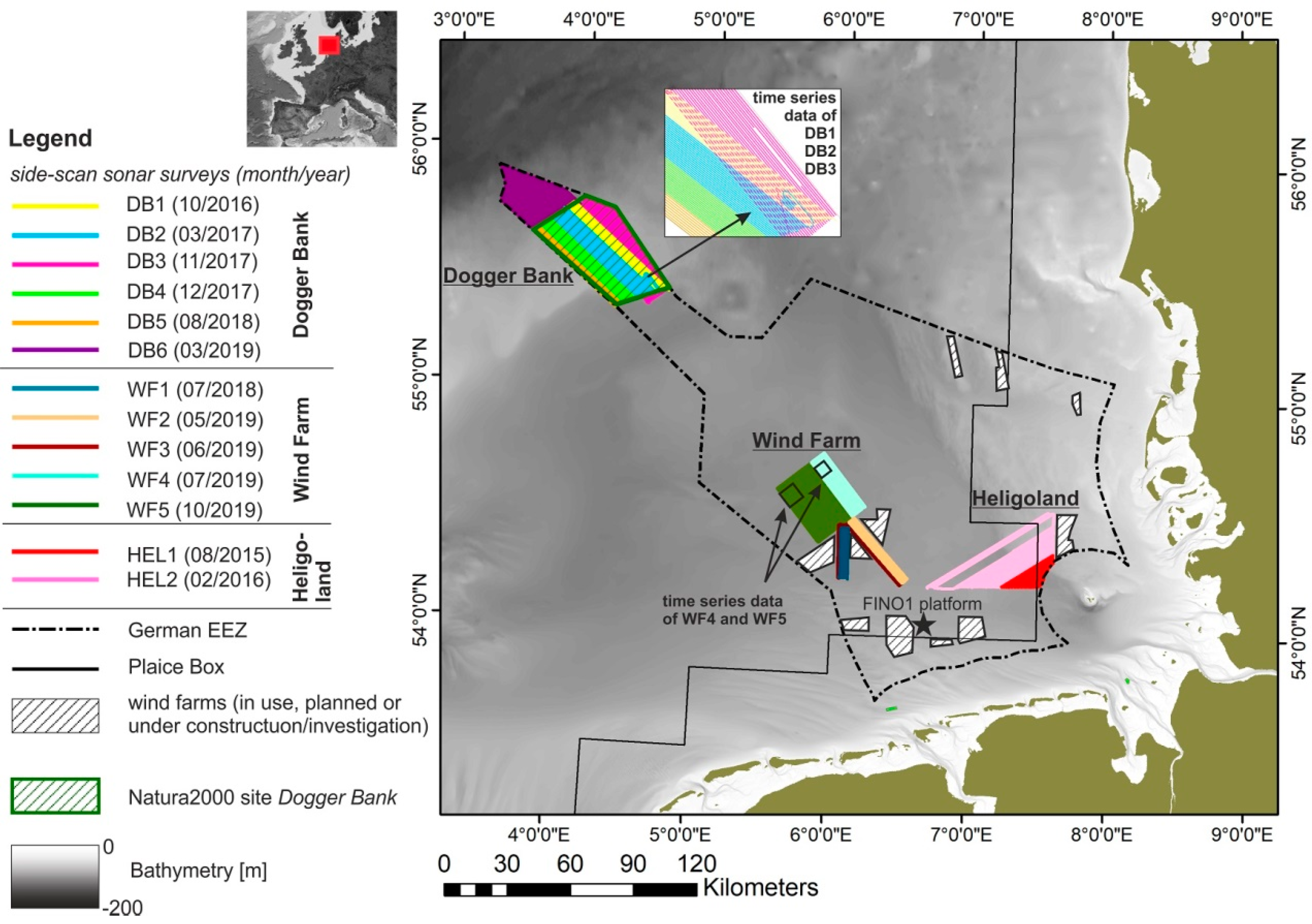
2.1. Study Sites and Physical Settings

The development and the actual sedimentary and morphological characteristics of the German North Sea have been mostly influenced by the late Pleistocene sequence of glacial and interglacial cycles. During the last glaciation (Weichselian), the glaciers did not reach the area of the modern German Bight but during the Saalian and earlier glacials, moraines and meltwater deposits were formed [32]. After the Last Glacial Maximum (ca. 10,000 y BP), the sea level began to rise and glacial/periglacial deposits were reshaped by waves and currents, which is still ongoing [33]. In the German Bight, Holocene sediments consist of the reworked glacial/periglacial materials, forming mobile sand layers and lag deposits [34]. The North Sea is a shelf sea and water depths in the German EEZ are increasing slightly from <10 m near the coast to >50 m in the north-westernmost part. In coastal sectors the hydrodynamics are mainly tide driven, whereas waves play a bigger role in the central part of the North Sea [35]. The distribution of sediments reflects such a hydrodynamic regime [36,37].

2.1.1. Study Site “Dogger Bank” (DB)

The Dogger Bank is a topographic height in the central North Sea where water depths are ranging between 20–40 m. Holocene sediments have thicknesses of 1–5 m, in some parts up to 30–40 m [38]. In this study the part of Dogger Bank, which is located in the German EEZ (known as “Tail End”, approx. 130 nautical miles north of the mainland) was examined. Here, water depths are between 35–40 m (Figure 1). Seabed sediments are mainly fine to medium sand with low mud content [39,40,41]. In 2004, the German part of the Dogger Bank was integrated into the international Natura2000 network for nature conservation (Figure 1). Due to its specific biodiversity, which is related to the high primary production rates, it is particularly worth protecting [42,43]. Hence, multi-lateral discussions on e.g., restricting bottom trawls and implementing enhanced enforcement regulations are ongoing and fishing may be restricted in the future in order to allow benthic species to gain biomass [44]. Currently, trawling is allowed within the DB study site and beam trawls (TBB) and otter trawls (OTB) are common [23]. Based on data from the vessel monitoring system (VMS), the fishing effort of was calculated for the German EEZ using the swept area ratio (SAR), which is the area that was touched by the trawl gear during one year normalized over the respective grid cell (0.05°*0.05° in this case) [45]. This means, an area equivalent to the grid cell was trawled during that particular year. For the years 2016 and 2017, the SAR for TBB was between 0.1 and 1.4 and for OTB it was between 0.1 and 0.9 in the area of the DB study site [45]. The fishing effort relies mostly on large trawlers (>221 kW and >24 m LOA) [22], which are towing gears with varying size. In general, common TBB widths are 5–20 m and OTB can have door spreads of up to >100 m [21].

2.1.2. Study Site “Wind Farm” (WF)

The area is located north of the offshore wind farms (“BARD offshore 1” and “EnWB Hohe See”; approx. 50 nautical miles north of the mainland) in the south-western part of the German EEZ (Figure 1). Water depths are 39–42 m and seabed sediments consist of sand to muddy sand [39].
The site directly borders several wind farms (planned and already completed, Figure 1). It is assumed that wind farms lead to increased fish abundance as fishing is prohibited and the fish migrate also to adjacent areas, which can increase the fishing effort near such vicinities [46].
At the WF site, the SAR ranged between 0.6–2.5 (TBB) and 0.2–1.8 (OTB) for the years 2016 and 2017 [45]. Here, also mainly large trawlers (>221 kW and >24 m LOA) are operating [22] with the related gear sizes (TBB: 5–20 m width; OTB door spread: up to >100 m) [21].

2.1.3. Study Site “Heligoland” (HEL)

The third study site is located approx. 13 nautical miles northwest of the island Heligoland (Figure 1). The water depth increases from northeast (25 m) to southwest (40 m) of the site. Coarser sediments (sands) are present in the northeastern part, whereas the mud content increases up to >10% in the southwestern part [39,41].
The HEL site includes a small area of the Plaice Box (Figure 1), which is closed for large trawlers (>221 kW and >24 m LOA). An increased fishing activity of large trawlers was observed at the borders of the Plaice Box and therefore also within the HEL site [23]. The SAR was up to 2.9 in 2015 (TBB). In 2016 and 2017 it was 0.1–1.3 (TBB) and 0.1–0.4 (OTB) [45]. The small trawlers (<221 kW, <24m LOA), which are allowed to operate within the Plaice Box, are equipped with smaller gears (TBB: 4–8 m width, OTB door spread: several tens of meters) compared to the large trawlers [21].

2.1.4. Bottom Contacting Trawling in the German EEZ, North Sea

In order to identify the TM, the different construction of the related trawl gears, which are common at the study sites (TBB and OTB), have to be considered.
TBB have a rigid beam to open the net and the mouth width of TBB is therefore constant (Figure 2). In order to move over the seafloor, runners (called “shoes”) are attached to each side. Ground ropes with additional tickler chains are fixed to the bottom side of the net in order to penetrate the first few centimeters of the substratum and startle demersal fish. In sandy and muddy sediments the penetration depth is <10 cm and TBB are often towed in pairs [21,22]. Most of the impact of TBB is induced by the ground gear as it affects the seabed surface and the subsurface [21]. In German waters, target fish for TBB are mainly demersal flatfish, like plaice and sole [23].
In contrast to TBB, the mouth width of OTB is variable. They have “doors” or “otter boards” attached to each side (Figure 2), which open the net and, according to the towing speed, control the mouth size (door spread). The doors of OTB are rather narrow compared to TBB and therefore have a greater penetration depth: <10 cm in sandy sediments and up to 35 cm in muddy sediments [21]. The impact of OTB is mainly produced on the surface of the seabed by the otter doors [21] and the width of an individual OTB mark is related to the door length and the angle of attack (Figure 2) [19]. OTB can be also towed in pairs, being called otter twin trawls (OTT), but this is rather uncommon in the study sites [22]. OTB target also demersal flatfish species as well as gurnard or sand eel [23].

2.2. Data Acquisition and Processing

2.2.1. General Survey Information

Within the framework of the “SedAWZ” project, SSS and ground-truthing data (grab samples and under-water videos) were used to create a sediment distribution map for the German EEZ [28]. Multiple surveys were carried out in recent years, which served as a base for the TM mapping and their description in this study. In order to provide a comprehensive mapping of TM, three study sites and a high number of surveys were selected (Figure 1), which allows it to point out spatial patterns of TM specific to the respective site. Two sites include time series data to investigate the degrading and the persistence of TM (sites DB and WF, Figure 1). Environmental factors (sediment type, water depth and related wave impact, fishing effort) slightly differ between the sites. Therefore, it was possible to examine the role of these factors in TM characteristics (spatial patterns, degrading/persistence) in each site. Further details of the individual surveys per study site are listed in Table 1:

2.2.2. Grain Size Analysis and Under-Water (UW) Video Recordings

In order to ground-truth the results from SSS data concerning the sediment type, surface sediment samples were obtained by means of Shipek and Van-Veen grabs (Figure 3) in the course of the “SedAWZ” project. The itemization of the sediment fractions (gravel, sand, mud), which was done for the present study, provides extra information to the prior known sediment distribution. In total, 158 samples (DB1 10 samples, DB2 9 samples, DB5 18 samples, DB6 26 samples, WF5 15 samples, HEL1 36 samples, HEL2 44 samples) were collected based on the real-time SSS data. The sediments were decalcified with acetic acid and organic matter was removed with hydrogen peroxide. For surveys DB1 and DB2, grain sizes were measured with a laser particle sizer (Table 1, LPS). The measurements for the rest of the surveys were done as follows: gravel, sand and mud fraction were separated via wet sieving. The grain sizes of the dried sand fraction were calculated from settling velocities by means of a settling tube [47]. For the mud fraction, X-ray transmission time series were measured by using a Micromeritics Sedigraph particle analyzer [47,48,49]. The mode (most abundant grain size in a sample) was averaged over the samples within each sampling site.
The UW-cameras (Table 1) were attached to a sledge operated in drift mode, without an active steering. The individual hauls (30 stations, Figure 3) were conducted for 5–10 min with a speed of ≤1 knot (ca. 0.5 m/s). Videos provide 48 frames per second (FPS) with 1920 × 1440 pixels (GoPro) and 30 FPS with 640 × 480 pixels (Kongsberg). The UW-videos were obtained in order to ground-truth the sediment type within the “SedAWZ” project and for the present study, they were examined regarding the detection of TM. The videos were not manipulated (e.g., with a video editing program) in order to enhance the image quality.

2.2.3. Side-Scan Sonar (SSS) Data Acquisition and Processing

The hydro-acoustic surveys were originally designed for seabed sediment mapping within the SedAWZ project, following the recommendations for an optimal combination among resolution, spatial coverage and time [28]. Hence, they were not specifically designed for investigating TM. The SSS was towed with approx. 5 knots (ca. 2.5 m/s) and the swath (300–400 m) and line spacing (300–400 m) were planned in order to cover at least 100% of the seafloor. Only for surveys DB3 and WF1 the coverage was of ca. 50%, due to limitations in survey time. Three SSS systems were used during the surveys (Benthos, Edgetech, and KLEIN, Table 1 and Table 2). Despite the slightly different technical characteristics, the systems are able to deliver comparable datasets. A minimum resolution (across and along track) of 1 m was achieved for all the surveys and datasets.
The quality of SSS data varies across the different surveys due to a combination of several factors. Environmental variables such as weather and sea condition, turbidity of the water, etc., change during the same survey and among the surveys, which influence the quality of the data (signal/noise ratio, backscatter absorption, presence of artifacts). The TM signature and its detection on SSS data are therefore affected by those factors. This is especially important for assessing the persistence and degradation of the TM. However, rough sea conditions were avoided during the surveys and SSS records were corrected in order to obtain reliable and comparable datasets.
The software SonarWiz6.05/SonarWiz7 (Benthos and Edgetech SSS systems) and SonarPro14 (KLEIN system) were used for acquisition. Automatic gain control (AGC) was turned off and time varying gain (TVG) was active. Post-processing was performed with SonarWiz7.01 applying the following steps:
  • slant-range correction
  • empirical gain normalization (in order to correct over- and under-amplified areas)
  • de-stripe filter (in order to remove artifacts due to tow-fish movements)
  • layback correction (in order to ensure precise positioning within the mosaic)
The resulting mosaics were exported at 1 m (=1 pixel) resolution. Changes of TM with time in terms of changing backscatter values were examined by calculating histograms (grey-level distribution of the pixels across the area) and corresponding statistics of six mosaics. The histograms were computed from the whole mosaics (see Section 3.5). For each pixel of the respective mosaic (raster data), a point feature was rendered with ArcGIS, containing geographic information and the backscatter value (0–255) of each pixel (=point). In this way, it was possible to use the histogram function of the Geostatistical Analyst provided by ArcGIS, which allows to display the graph as well as to derive lower- (mode, standard deviation) and higher-order statistics (skewness and kurtosis).

2.2.4. Multibeam Echo Sounder (MBES) Data Acquisition and Processing

In order to describe the morphology of the TM, high resolution bathymetric data were collected simultaneously with the SSS records by means of a Kongsberg EM710 MBES. The system is permanently mounted aboard the RV Heincke and coupled with a PHINS (Photonic Inertial Navigation System) motion sensor for pitch, roll, heave, and yaw real-time compensation. SVPs were used for sound velocity calibration, and positioning was achieved by means of a DGPS system. The MBES operates at frequencies of 70 to 100 kHz and with an opening angle of 65°. A swath width of approx. 120 m (ca. 4× water depth) was achieved. For the present study, a subset of the data was further processed using the Multibeam Imagery tool from SonarWiz7.01. The resulting grid has a lateral resolution of 0.75 m. A non-optimal correction of the vessel motion is likely responsible for the artifacts in the external parts of the swath and for the general bathymetric “noise”, which affected the final outcomes. However, the general aspect and the morphometry of the TM could be detected.

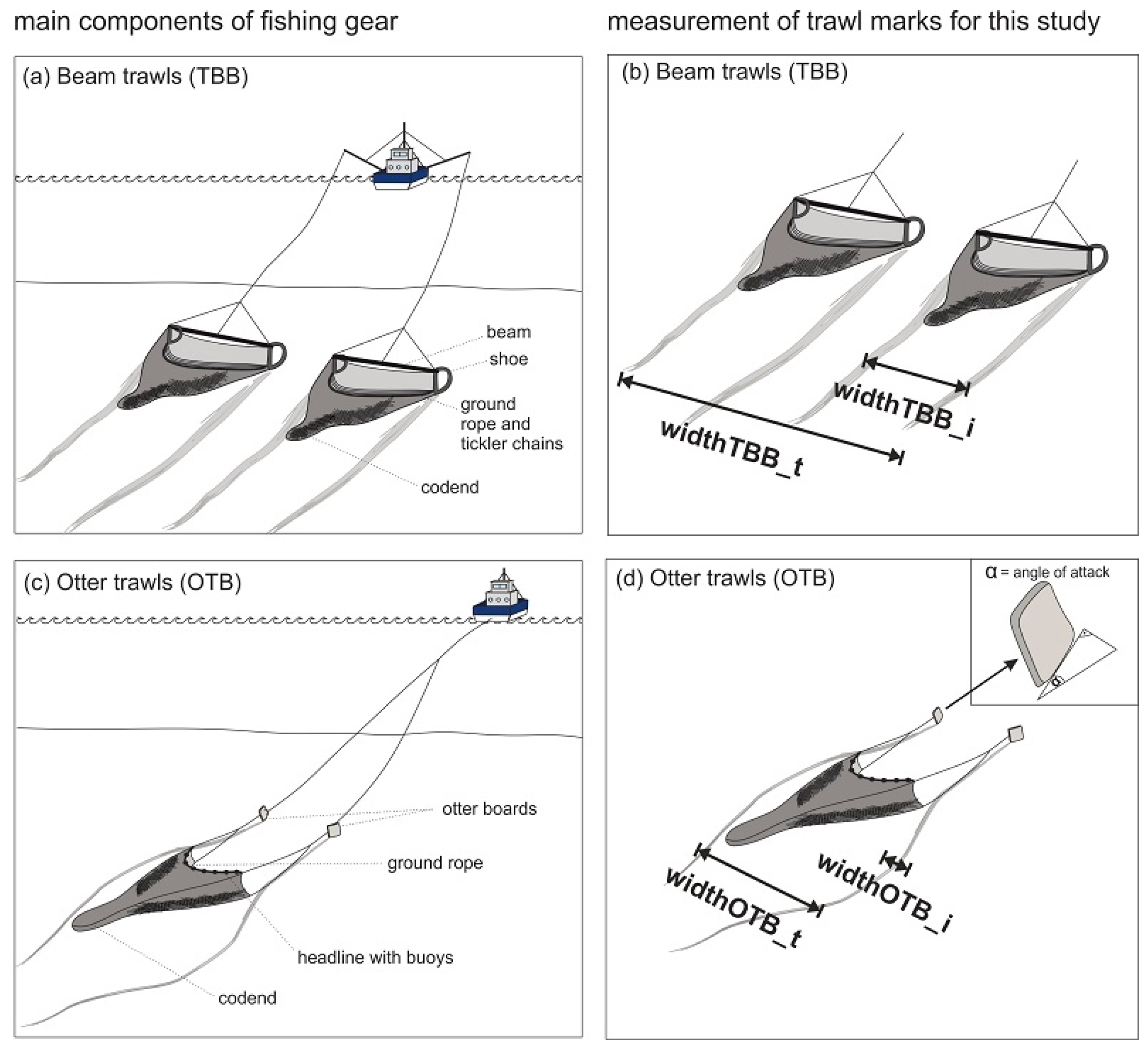
2.2.5. Trawl Mark Mapping

For each study site the TM were manually mapped (i.e., digitized) from the 1 m resolution SSS mosaics and stored as ESRI-shapefile (polyline). TM were classified according to the trawling gear type, based on their different patterns in the SSS mosaics: TBB marks show a constant width all along the course of the track, due to the fixed mouth size; in addition, they are towed in pairs (Figure 2a). On the contrary OTB marks are rather narrow and present irregular patterns as the door spread differs in width (Figure 2c). For each gear type a shapefile was created for the respective survey. The number of mapped trawl marks is influenced by the SSS data quality. As stated earlier, the SSS data quality changes across the surveys and TM might be not detected due to artifacts caused by e.g., turbulences in the water column. Therefore, the mapped TM represent a minimum number (and density).
Files were merged for each study site and the azimuth (trawling direction) of the TM was calculated, in order to point out potential preferred trawl routes. Hereafter, the direction is given in a bidirectional manner (e.g., NW-SE, implying both directions are possible) because the heading of the vessel cannot be derived from TM. The azimuth calculation was done by means of the ArcGIS field calculator and the results are displayed as rose diagrams (Figure 4).
In addition, TM files were merged according to gear type (=neglecting the survey information and study site) showing the overall density for both TBB and OTB. With the help of the “line density” ArcGIS function a TM density distribution was rendered, with a grid resolution of 1 × 1 km. Such function counts the occurrence of lines within a given radius (1 km in this study), regardless to the length of the individual TM. This means that a grid cell can show low TM density although the area touched by the trawl gear is high due to few but long-distance TM. By comparing the line density values of the surveys, the relative changes in the fishing intensity can be resolved.
In order to further determine the geometry (i.e., metrics) of TM from the corresponding gear type, 100 TM were randomly picked from the SSS data of each study site and specific metrics were determined (Figure 2):
  • width of individual TBB mark was measured (widthTBB_i)
  • total distance from starboard to portside TBB (widthTBB_t)
  • distance between the otter boards (door spread, widthOTB_t)
  • width of the marks created by the otter doors (widthOTB_i)

2.2.6. Observation of Fishing Vessels

In the course of surveys DB1, WF4, and WF5 operating fishing vessels were observed, which allowed to immediately record new TM and thus determine their date of origin. An estimation of the persistence and an investigation of potential signs of degradation of TM at the study sites DB and WF was possible by performing re-surveys:
  • DB1: observation of a single vessel, re-survey after five months (DB2)
  • WF4: observation of a single vessel starting a new haul, re-survey after 36 h
  • WF5: observation of multiple vessels, re-survey after six days including three days of rough sea conditions (significant wave height approx. 4 m)

3. Results

3.1. Sediment Types—Grain size and UW-Video Analysis

The DB site is dominated by sandy sediments (mode = 177 µm) with a mud content of ≤5% and ≤1% of gravel (Figure 3a,c and Figure 5a). Only in the northernmost part, gravelly patches are occurring and the gravel content increases up to 75% (Figure 3b and Figure 5a).
Similarly, the WF site is dominated by sandy sediments (mode = 149 µm) and the proportion of mud is slightly lower in the northwestern part (5–10%) than in the rest of the area (mud content up to 23%, Figure 3d and Figure 5b). Gravel is absent in all samples.
The HEL study site shows slightly coarser sand than at the other sites: mode = 210 µm with <5% mud and without gravel in the northeastern part (Figure 5c). In the central part, there are patches with high gravel content (20–40%, Figure 3e and Figure 5c), and the southwest is characterized by an increase in mud content (10–20%, Figure 3f and Figure 5c).
UW- video analysis from DB site confirmed the findings from the backscatter data (in terms of sediment-type) and grain size data. The picture shows sand with occasional shell deposits and ripples with approx. 10 cm wavelength (Figure 3c). For the other sites, no UW-video is available (Table 1).

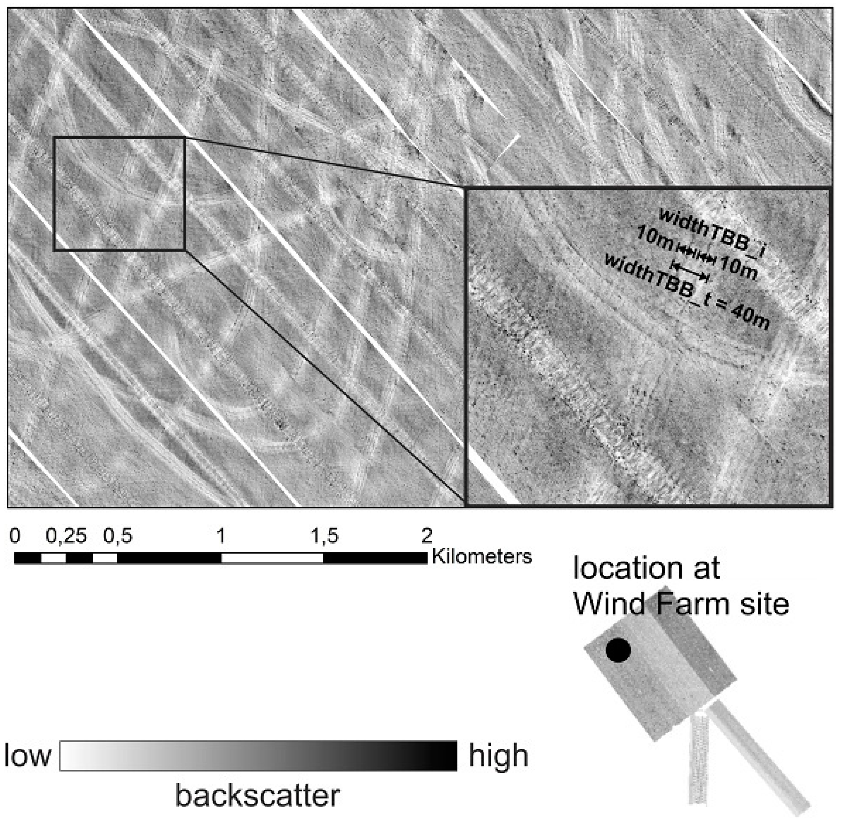
3.2. Acoustic Signature of Trawl Marks

The mapping revealed that TM have different levels of visibility in backscatter data. In some cases, they are not clearly distinguishable from the background (Figure 6a), and in some cases they appear rather distinct (Figure 6b, TBB mark of the observed vessel, DB1). Moreover, TM appear with different backscatter values depending on the study site: At the DB site, TBB marks, compared to the surrounding sediments, show higher backscatter values in their center, which is bordered by slightly lower backscatter (Figure 6b and Figure 7b). This detailed backscatter signature is not always present. TM can appear with higher backscatter (compared to the surrounding) over their whole width (Figure 6b) as well, which is most commonly observed in clustered TM.
TBB marks within the WF site mostly show the detailed backscatter signature but the lower backscatter parts are more pronounced compared to TM at the DB site (Figure 8).
OTB marks could be identified in SSS data only at the WF study site. They show lower backscatter in the center and higher backscatter at the outer, signal facing edge (Figure 9).
Regarding the backscatter signatures of TBB marks at the HEL site, they are characterized by higher backscatter in the northeastern part of the site and with lower backscatter compared to the surrounding in the southwest (Figure 10). The former also show a detailed signature, similar to TBB marks at DB site.

3.3. Trawl Mark Geometry and Morphology

Based on the specific pattern shown in the backscatter data, it was possible to differentiate between TBB and OTB marks: two parallel marks with 10–12 m width (widthTBB_i) and an average distance of ca. 40 m (widthTBB_t, Table 3, Figure 7) were classified as pair-towed TBB marks. Slightly smaller TBB marks (9.5 m on average) were found at the HEL site (Table 3). At the WF study site, highest widths of TBB marks could be measured (mean ca. 11 m, Table 3).
Similar could be observed on the bathymetric data: TBB marks appear as parallel tracks and show a distance of 30–40 m and an individual width of 8–12 m. Figure 11 shows an example of such marks with both straight and curved forms. The TBB marks are slightly depressed (5–10 cm) with respect to the surrounding areas.
OTB have a variable door spread and therefore produce rather irregular patterns compared to TBB tracks: In this study, OTB marks could only be recognized at the WF study site and semi-parallel marks have distances (i.e., door spreads, widthOTB_t) up to 281 m (126 m on average) and the individual marks created by the otter boards are ca. 3 m wide (widthOTB_i, Table 3, Figure 9).

3.4. General Trawl Mark Mapping

As the bathymetry is quite gentle in all three study sites (Figure 4), a significant relation between water depth and TM density could not be found. The main orientation of the TM is NW-SE and N-S (Figure 4).
TM could not be observed in UW-video recordings, although TM density was very high, e.g., during survey DB1 (October 2016, Figure 4, Figure 12).
In the DB2 dataset a TBB track was mapped in the E-W direction for roughly 10 km, crossing the entire SSS mosaic (Figure 4, DB1). Similar to the DB2 survey, several consecutive TBB tracks of approx. 12 km length were observed across the whole SSS mosaic collected during the DB3 survey.
Mapping also revealed that TM can occur as consecutive tracks or clustered (Figure 4), which is however difficult to differentiate at locations were TM density is high and individual TM are strongly overlapping, or when TM are poorly preserved.
The spatial density (“line density”) of TM changes between the different surveys (i.e., months) as it can be seen at DB site: the highest density of TM could be observed in surveys DB1 and DB5 (October 2016 and August 2018, up to 20 counts per km2, Figure 12), the least in DB3 (December 2017, 2–4 counts per km2, Figure 12). Within the WF study site, TM density is highest in July 2019 (WF4) and survey WF5 from October 2019 (up to 20 counts per km2, Figure 12). In contrast to the other study sites, OTB marks were recognized at the WF site, but with lower density (max. 5 counts per km2, Figure 12) compared to TBB marks. The HEL study site shows highest densities in August 2015 (HEL1, up to six counts per km2), whereas counts were ≤4 per km2 in February 2016 (HEL2, Figure 12). OTB marks are absent here as well.

3.5. Trawl Mark Preservation and Potential Signs of Degradation

Surveys DB1, DB2 and DB3 overlap in the southern part of the DB study site (Figure 1). The resulting time-series data collection took place after five (DB2) and 13 (DB3) months (Table 1) from the first dataset. None of the previously mapped TM was still visible in the later SSS datasets.
The TBB marks in Figure 13a could be dated to the period of the 22–24 October 2019; fishery was active at the same time as the SSS survey. SSS data of the re-survey show a decreased visibility of the TM: the “new” marks were clearly to follow and showed details, whereas “old” TM can be identified but appear rather pale and blurry (Figure 13b). The histogram of the mosaic with the “old” TM (Figure 13b) shows a higher standard deviation (σ = 19.27) than the mosaic with “new” TM (σ = 14.06, Figure 13a). The skewness was calculated to be −0.91 for the initial mosaic and −1.23 for the second. The mode of the grey values of the “new” state mosaic is 172 and the mode of the “old” state mosaic it is 177. The kurtosis did not change between the two mosaics (leptokurtic distribution, 7.13).
On the SSS-record in Figure 14, a V-shaped pattern of TM is visible, which was classified as OTB mark. High backscatter values and corresponding acoustic shadow clearly define these TM regarding the background. When the TM were surveyed again, the transition to the surrounding sediments was rather gradual: The TM showed lower backscatter compared to the surrounding and the high backscatter parts were absent. The corresponding backscatter histograms reveal a shift of the standard deviation (σ) from higher to lower values for both SSS frequencies (Figure 14). The skewness is clearly negative (−1.39 and −1.06) in the mosaics of the first survey and changes to values near zero for the mosaics from the second survey (−0.31 and −0.15). The distribution is leptokurtic and shows higher values (7.5 and 9.04) for the initial mosaic and decreases to 4.02 and 4.23 in the second. The noise caused by the propeller and wake of the fishing vessel (Figure 14a,c) is also absent in the second survey (Figure 14b,d).

4. Discussion

This study revealed differences in TM density among the individual surveys. The highest spatial density of TM was found in the surveys of the summer months (August and October). Fishing activity depends on the abundance of target fish as well as weather conditions. Kaiser et al. [51] also found the highest density of trawling activity in early summer to summer due to the opening fishing season in the Irish Sea. In the German EEZ, the largest catches of plaice and sole (targeted by TBB and OTB) are mostly observed within the 3rd and 4th quarter of the year [22]. Storms are most common in the winter and therefore these months are expected to show the least amount of TM. For instance, storm “Herwart” [52] affected German waters with significant wave heights (Hs) up to 8 m and wave periods (T) between 10 s and 15 s at the end of October 2017 [50]. It is suggested that the wave-base reworks the seabed during winter storms and the TM are flattened faster compared to summer, which could explain the relatively low density of TM detected in November and December at the DB site. The effective wave-base reaches about twice as deep during stormy weather than under normal weather conditions, even during a mild storm (Hs = 2.4 m, T = 6 s) [53,54]. Gilkinson et al. [18] found that winter storms (for Hs > 6 m at 67 m water depth on the Scotian Shelf) are the main reason for sediment reworking, causing degradation of TM.
In this study, TM were hardly to distinguish from the background in some cases (Figure 6a). The limited traceability produces an error in overall TM density, which is hardly to quantify as trawling is not equally distributed but can overlap [55,56]. Hence, the density measure (line density), which is presented in this study cannot be understood as an absolute measure of trawling intensity and, moreover, it reflects a minimum density as stated earlier (see Section 2.2). TM are often not visible in the far range of the SSS swath, which is most prominent at DB site (Figure 6b). It is estimated that, on average, one third of a TM is not visible due to this problem. This, however, does not contribute to an error in TM spatial density, because the length of TM is neglected in the calculation.
The main orientation of the TM in the study sites is WSW-ENE (DB site), N-S (WF site), and WNW-ESE (HEL site, Figure 4). Malik and Mayer [25] as well as Smith et al. [15] describe that trawling is often conducted parallel to isobaths, which generates a bathymetry-related orientation of the TM. In our study, the bathymetry is rather gentle (Figure 4) and the orientation of the TM is therefore independent from the water depth. In the study sites, wind and waves are mainly westerly oriented (NW, SW, [37]) and tides northerly [37], which could explain the preferred bearings of the fishing vessels.
At sites DB and HEL, TM are oriented approx. W-E and are rather perpendicular to the acoustic data collection grid (Figure 4). In SSS data, elongated features such as cables and pipelines are more likely to be detected if orientated along tracks [57]. The survey direction plays therefore no significant role in the detection of TM in these areas. However, at WF site TM have mainly N-S orientation, which is parallel or sub-parallel to the survey direction (Figure 4). OTB marks that are only found at the WF site could be more sensitive to directionality of the SSS-signal because they are rather narrow. This would result in missed OTB marks perpendicular to the survey direction, affecting the measure of density in Figure 12 and making the comparability of TM spatial density between the sites difficult. Enhancing acoustic shadows and increasing across-track resolution by towing the SSS nearer to the seafloor and/or narrowing the swath could, moreover, have improved data quality and therefore TM detection.
TM could not be detected in UW videos, despite the high spatial density of TM in some of the surveys (e.g., DB1, Figure 4, Figure 12). Malik and Mayer [25] reported similar results for the Gulf of Maine (<100 m water depth), due to the limitations in the camera steering options and in the positioning (mismatch between the TM detected in the acoustic data and the camera positioning). The camera system used in this study captures only a section of the seafloor (ca. 1 m2), likely too small in comparison with the TBB mark widths (>5 m). Moreover, a steering option would probably increase the chance to catch TBB on UW footage. In addition, the ripples in the DB study site indicate sediment movement due to currents and waves and their size is similar to the penetration depth for TBB in sandy sediment (≤10 cm, [21] and Figure 11), which further complicates TBB mark identification.
In contrast, Mérillet et al. [16] observed TM on UW-videos (sledge-mounted camera, no active steering). However, they examined OTB marks in rather muddy sediments (sand, muddy sand, and mud), which were <0.5 m wide (furrows created by otter boards). This could have influenced the visibility of TM in UW-video footage as narrower OTB marks could be resolved more easily by a camera section of 1 m2. Smith et al. [15] detected TM in UW-video footage on muddy but not on sandy seabed (visible in SSS-data in both sediment-types). Gilkinson et al. [18] described that TM created by a hydraulic dredge (uses cutting blades and water injections instead of tickler chains) are detectable in UW-videos of sands (primarily medium grained) in 65–75 m water depth but after one year they were not detectible in UW-video material anymore while they were still visible in SSS data up to three years. This supports the assumption that the gear penetration at the DB site is too low or the TM are too old (i.e., flattened) to have the furrows detected with UW-video.

4.1. Acoustic Signature of Trawl Marks

TBB marks show higher backscatter values in their center and lower backscatter values at their edges, compared to the surrounding sediments (Figure 15). In the WF site, the low backscatter area is more pronounced (Figure 15) and in some parts of the HEL site, high backscatter in the center of TM is completely missing (Figure 15). That can be explained with the reworking of the sediments due to the trawling gear: fine grained, silty material gets re-suspended during trawling and settles in the furrow and the adjacent areas, which was also described by Gilkinson et al. [18]. This would result in lower backscatter (smoother surface) compared to the surrounding sediment. Depending on the local hydrodynamics, bottom currents can instead transport the material away and settle it down elsewhere, which was described by Palanques et al. [58] and Mengual et al. [59]. As a result, they observed a coarsening of the sediments along the trawled tracks, due to the removal of the fine-grained fraction (silt to clay). Where the seabed consists of coarser sediments, like at the DB site and in the NE part of the HEL site, (with >90% of sand, Figure 5) such a fine sediment removal is less pronounced, as the mud fraction is nearly missing. In these areas, the increase of the backscatter values in the center of the TM is therefore due to the mechanical interaction of the trawling gears with the seafloor. Feldens et al. [60] could show that lower frequencies (200 kHz in this case) are able to increase the detection of specific seafloor features (e.g., when they appear rather subtle), which can be assigned to different contributions of volume and surface scatter, and texture to the backscatter signal. Similarly, it was observed that TBB marks in survey DB5 were more evident in the 100 kHz than in the 400 kHz SSS frequency records. This should be examined further.

4.2. Trawl Mark Geometry and Morphology

Different trawl gears could be assigned to the TM in the SSS backscatter showing significantly different patterns and metrics. TBB marks appear in rather regular and parallel-like patterns compared to OTB marks, as already described by Eigaard et al. [21]. The beam widths (widthTBB_i) range between 4 m and 22 m in our study sites (Table 3), which corresponds to fishing vessel engine power of 200–900 kW for TBB trawler targeting demersal fish [21]. Large beam trawlers (>221 kW) are active in all three study sites, whereas small beam trawlers (<221 kW) are operating mainly within the 12-nautical-mile-zone and, less frequently, also NW off Heligoland within the EEZ [22]. Therefore, TBB marks at sites DB and WF were likely made by large beam trawlers catching demersal fish. According to their size, TBB marks at the HEL site were probably created by a mix of large and small beam trawlers.
In regard to the otter trawlers fishing in the North Sea area, a door spread of approx. 50–300 m occur corresponding to vessels of 10–40 m LOA [21]. A maximum door spread (widthOTB_t) of 281 m and a mean door spread of 126 m (Table 3) were measured at the WF site. Such wide door spreads occur in fleets targeting demersal fish and mixed bentho-pelagic species, while smaller door spreads are usually used for catching crustaceans, sprat or sand eel [21]. Individual OTB marks in this study present widths (widthOTB_i) ranging from >1 m to 6 m with an average of approx. 3 m (Table 3). Lucchetti and Sala [61] noticed widths of 30–40 cm in the Mediterranean Sea. Krost et al. [19] described OTB marks with widths of <1–2 m in the Baltic Sea and related them otter door lengths of approx. 2 m, considering the angle of attack (ca. 30°). Lucchetti and Sala [61] mentioned a door spread of <50 m and Krost et al. [19] related the observed OTB marks to small fishing vessels, which probably use smaller gears. It is likely that higher door spreads in the present study are caused by larger nets and otter doors than in the other studies, which could explain the discrepancy in widths of the door marks. Sala et al. [24] found maximum door spreads of 292 m (mean 90 m) in a vessel and gear metrics database of the Mediterranean Sea. Otter board lengths were approx. 3 m (mean 1.9 m), which would result in a furrow of 3.5–4 m width, assuming an angle of attack (Figure 2) of 30–40°. This is in accordance with the findings of this study; OTB marks have mean widths of 3 m (Table 3).
As expected, OTT marks could not often be identified in backscatter data as OTT fishing is quite rare compared to the other métiers [22]. One example which is probably an OTT mark could be found (Figure 14). Due to the fact that the corresponding vessel was observed, the TM could be assigned to a single haul but if the TM would have been observed without context it also could be interpreted as two single OTB marks with more or less the same bearing. Overlaps of fishing routes of individual vessels or within fleets is not uncommon [55] and therefore OTT/OTB might be overseen.
Malik and Mayer [25] found trawl tracks of >12 km length corresponding to a 6–8 h haul at 2–3 knots trawling speed. The trawling speed is approx. 5 knots for TBB catching demersal fish [62], which can produce a consecutive trawl track of >50 km length for a 6 h haul. In this study consecutive tracks of approx. 10 km length were found in all three research sites but their length is limited by the SSS covered area and by the orientation of the TM respect to the collected dataset. Some TM could only be followed over distances of <1 km, which is also reported by Malik and Mayer [25] as connected to scallop dredging. However, VMS data show that dredges for scallops are only used in coastal waters in the German North Sea [22]. As a consequence, the shorter tracks can rather be related to limited traceability due to difficulties in distinguishing TM from the background, SSS survey size and the occurrence of low spatial density clustered TM in consequence of degradation.
Exemplary MBES data from survey DB1 show a morphological change of <10 cm in a TBB mark (Figure 11). Bathymetry data show TBB morphologies of a similar size and aspect to the SSS records. The shoes of the TBB should produce depressions in the seafloor, bordered by centimeter scaled ridges due to the sediments pushed away by the shoes. On the bathymetric data such a sequence (ridge-depression-ridge) could be observed, although the miscompensation of the motion sensor and the resulting morphological artifacts do not allow a clear distinction of those geometries respect to the “bathymetric noise”. The TM are clearly more evident in the SSS than in the MBES records. The morphological change of the TBB marks (Figure 11) is in accordance with Eigaard et al. [21], where a penetration depth of <10 cm was stated for TBB on sandy sediments. Depestele et al. [7] described changes in seabed bathymetry of 2–6 cm caused by a 4.4 m wide TBB on a sandy sediment (median grain size 144 µm). This change is slightly less than observed in the data of the present study, which can be explained by the size of the gear; the TBB mark (Figure 11) has a width of approx. 10 m and therefore the related gear is assumed to be larger and heavier. However, multiple passages of the trawl gear can also increase the morphological change [7]. If the TBB in Figure 11 was created by multiple gear passages is unknown but the ridge-depression-ridge sequence would probably have another form (e.g., more than two ridges) because it is considered unlikely that the gear passed the exact same track multiple times.

4.3. Persistence of Trawl Marks and Signs of Degradation

TM preservation varies based on multiple factors like sediment type, hydrodynamics (e.g., tidal currents, waves, storm events) and trawling patterns. In this study, a minimum preservation time of 5–7 days and a maximum preservation time of <5 months could be defined in the DB site: Several TBB marks were observed across the whole SSS mosaic of DB2 and as the data collection spanned between 9th and 13th March 2017 (DB2), it is reasonable to assume a minimum preservation time of roughly 5 days at this location. In DB 3, similar to DB2, several TBB tracks of approx. 12 km length were identified, which corresponds to seven days survey time (Table 1). The same order of magnitude for minimum preservation time of TBB marks could be observed at study sites WF (TM of ca. 10 km ≙ five survey days) and HEL (TM of ca. 7 km ≙ four survey days). During the DB1 survey, a trawling vessel was real-time observed during fishing operations. The TM was recorded (Figure 4 and Figure 6b) and re-surveyed during DB2 (March 2017). It could not be identified again, which means the maximum preservation time is <5 months at this site within the investigation period. Lindeboom and de Groot [5] described a preservation time of 52 h in coarse sand in the southern North Sea, using a smaller beam trawl (4 m beam width) deployed in shallower water (approx. 15 m water depth), which could explain the shorter persistence compared to results of this study.
Mérillet et al. [16] observed that bioturbation could lead to a lower persistence of TM. In general, bioturbation is higher in muddy than in sandy sediments [63], therefore, bioturbation is likely not a significant controlling factor for the preservation of TM in the three study sites, where sediments are mainly made by sand with a very low mud content. However, in their model, Zhang et al. [63] described a pattern of increased bioturbation activity at Dogger Bank during summer. As a consequence, the TM at the DB site should be less stable during summer months, which is in contrast with the highest TBB mark densities recorded in that period in our datasets.
In the present study, it could be observed in SSS data that TBB marks can show a detailed backscatter signature (higher backscatter values in the center and lower backscatter values at the edges, Figure 15), whereas other TBB marks do not (clustered and blurry TBB marks, Figure 6a). The absence of these detailed patterns seems to be related to the progressing degradation of TBB marks and therefore, consecutive TM with a detailed backscatter signature are suggested to be rather “new” than clustered TM without these details. However, it has to be noted that differentiating between a “new” mark with low penetration and an “old” mark with high penetration is not possible [15]. For instance, electric pulse trawls have gained importance, e.g., within the Dutch fleet, which use electric pulses instead of the heavy tickler chains [64]. Thus, the gears have lower weights compared to conventional TBB, resulting in a lower penetration depth [65].
The evaluation of degradation and persistence of TM has to consider the limitations of the SSS system: The “new” TBB mark in Figure 6b can be traced across the whole SSS swath but neighboring TM are not visible in the far range of the SSS swath as most of the energy of the SSS signal is returned from areas closest to the source and the resolution decreases in the far range due to the angle of incidence and the signal travel time [66]. The size of the TM in respect to the SSS mosaic resolution plays also an important role. As the TM vanishes, their size is expected to reduce and therefore to be less detectable at the given SSS resolution of 1 m.
As expected, post-storm TBB marks from survey WF5 were less prominent (i.e., they were characterized by a lower backscatter intensity) and therefore more difficult to be distinguished from the surrounding sediments (Figure 13a,b). By considering the corresponding histograms, it could be found that the mosaic, which is displaying “new” TM has a lower standard deviation regarding the grey values (σ = 14.06, Figure 13a), than the mosaic with “old” TM (σ = 19.27, Figure 13b), indicating a lower contrast in the mosaic of the initial survey. This is unexpected because the contrast should decrease when TM are less pronounced. The skewness is showing a more negative value in the re-survey mosaic (−1.23; initial mosaic −0.91) and therefore the majority of the values within the distribution shifts in the direction of lower backscatter values (=“whiter” grey values) of the mode (176), although the low backscatter values of the TM are missing. This counter-intuitive change of the grey value distribution can be explained by lower data quality of the re-survey due to slightly rougher sea conditions compared to the initial survey (Figure 13c), resulting in an increased number of artifacts. It is hardly to quantify on which extend the data quality influences the change among the histograms. However, the subjective comparison (examination with the naked eye) of the two mosaics suggests that the TM are significantly less evident in Figure 13b.
Gilkinson et al. [18] described an “initial decrease in sharpness” of TM (4 m wide dredge) after the first year of observation followed by a “more gradual degradation of the tracks and their edges” in the next years until they were undetectable after three years in the SSS data (0.25 m resolution) of the mobile sand sheet on the Scotian Shelf in 65–75 m water depth. The authors concluded that storms are of major importance regarding sediment reworking. TBB marks at our WF site were hardly visible in SSS data after six days including three days of rough sea conditions (Figure 13). Gilkinson et al. [18], moreover, noticed a reversal in backscatter (from lower to higher compared to the surrounding) during the degrading process. In the present study, all TBB marks at the DB site show similar backscatter values (i.e., higher) compared to the surrounding. This means they either all have to be of the same age at the time of the survey or the effect of backscatter-reversal does to apply to our study site. At site HEL, both cases are present (high and low backscatter compared to the surrounding) but the high backscatter TM occur in coarser sediments than low backscatter TM, which likely depends on sediment-type rather than on the degrading processes.
The TM in Figure 14 shows a V-shaped pattern, indicating the proceeding divergence of the gear due to increasing vessel speed. High backscatter values with a corresponding acoustic shadow are clearly visible in the course of individual TM (Figure 14a,c), indicating pushed up sediments followed by morphological depressions. The high backscatter features at the ends of the individual furrows (i.e., TM) are interpreted as otter boards. It is assumed that this signature is related to an OTT, as the two nets share one otter board in their middle (=3 otter boards in total, [21]). Within 36 h, the morphological change vanished to the state, which is shown in Figure 14b,d. The standard deviation (σ) calculated from the histograms shifts from higher (Figure 14a,c) to lower values (Figure 14b,d). This indicates a decrease of contrast, which is likely due to the flattened TM with less pronounced acoustic shadows and the absence of the artifacts caused by propeller noise of the fishing vessel. In the mosaics of the initial survey, the grey value distribution is clearly negative skewed (−1.39 and −1.06), indicating that the majority of the grey values are concentrated right of the mode (158 and 170), i.e., around lower backscatter values (=“whiter” grey values). In the re-survey mosaic, the skewness is closer to zero (−0.31 and −0.15) and the distribution, therefore, is now concentrated nearer around to the mode (157 and 161). This seems reasonable, as the artifacts are missing and the TM has decreased in contrast. The kurtosis in the re-survey mosaics (4.02 and 4.23) is rather comparable to the normal distribution (kurtosis = 3) than in the initial mosaics (7.5 and 9.04), which is, as well, likely due the absence of artifacts and contrasts in the TM. Due to the striking artifacts (propeller noise) in the initial mosaics, it can be assumed that this contributes considerably to the change among the histograms. The subjective comparison (with the naked eye) of the mosaics, however, reveals rather gradual edges of the TM after 36 h, indicating a degraded TM.
Depestele et al. [7] reported that the TM of a 4.4 m wide TBB hardly changed their aspect after 12–44 h and a 4.4 m pulse trawl (similar to TBB but uses electric pulses instead of tickler chains) faded after 55–107 h. They conducted their studies in coastal areas (15–22 m water depth, median grain size 144µm) where tidal and wave related currents are more pronounced than in the three study sites. Nevertheless, the preservation time of the OTT marks observed in this study is even shorter. The degradation rate seems to be more dependent on the gear type and on the size (i.e., weight).
Palanques [58] observed OTB marks in muddy sediments on the Ebro Shelf (20–70 m water depth): these TM did not show any changes after a few days but after a year they appeared with lower backscatter values. They related the relative longevity to the cohesive properties of the muddy sediment (mud content >60%). In the WF study site, the mud content is relatively low, while it is likely that the altering of the OTT mark is faster.
At sites DB and HEL, any OTB mark was detected, whereas at the WF site OTB marks were present. The fishing activity related to OTB trawls is reported to be similar at all the three study in the years 2016 and 2017 [45]. Therefore, either OTB marks are not detectible in the DB and HEL sites or fishing did not take place during and/or before our survey. Similar to TBB in offshore waters, OTB fishing is targeting demersal flat fish. In this study, high relative TBB densities in the months of general high fishing activity (i.e., summer, Figure 12) were recorded and it is expected that OTB fishing is conducted at the same times because the gears are targeting similar fish populations. Consequently, it is likely that OTB marks were not recorded because the relative narrow furrows were masked by TBB marks and/or OTB have, compared to TBB, lower penetration depths in sands [21] and therefore the preservation potential of the marks is lower. In addition, the otter boards can float within the water column or touch the seabed at irregular intervals [28]. This leads to characteristic “dashed line-patterns” (Figure 9a), which makes the tracking of OTB marks over longer distances more difficult.

5. Conclusions and Outlook

Together with the detailed description of TM patterns specifically related to different trawl gears, the mapping presented in this study provides an insight into the physical disturbance on the seabed caused by bottom contacting trawling, which can help to evaluate the impact of fishing activities on sediments, seafloor morphology, and macrobenthos (flora and fauna).
In general, fishing activity maps are derived from positioning and logbook data of fishing vessels (VMS data, [67]). These data are usually aggregated over one year, if using SAR [45,67] and no further distinction about specific time windows is possible (e.g., seasons). SSS data can therefore provide additional and valuable information on a higher timely resolution concerning the fishing effort and its potential seabed disturbance. However, collecting recurrent (yearly or monthly) SSS datasets over large areas is very cost intensive and time consuming. Thus, it would be beneficial to examine potential advantages of the direct connection of SSS and VMS data in order to improve monitoring programs.
The present study reveals seasonal changes in the spatial density of TM: It was highest in August and October and lowest during the winter months (November to March, Figure 12) and TBB marks could be identified in all sites. Although the fishing effort for both gears is similar, OTB marks, surprisingly, only appear at WF site. This is probably related to a reduced persistence of OTB marks in sands as well as limited detectability in SSS-data due to their metrics, which is especially important if the quality of the backscatter data is not constant; the detection of narrow TM is rather difficult in rather “noisy” data. Moreover, the visual examination of backscatter data for TM mapping and descriptions strongly depends on the editor. Therefore, methods to reduce the “noise” in SSS data should be applied as well as standard guidelines and/or automated feature detection approaches are needed in order to improve the robustness of TM detection.
The extensive mapping of TM was based on approx. 4800 km2 of SSS data. SSS has the advantage of a wider swath (e.g., 400 m in this study) compared to MBES (e.g., 120 m in this study), which allows to survey an area with 100% coverage in a shorter time using SSS. In this study, TM were more evident in SSS than in MBES data, which is, however, likely due to the quality of MBES data. The carefully application of MBES data corrections by means of vessel motion and SVPs is therefore important in order to get more reliable morphometric measures, because the depth information is a great benefit of MBES. This could also help to identify the mechanical impact of the different gear parts (tickler chains and shoes). Moreover, a comparison of the backscatter data from both systems (SSS and MBES) would allow it to investigate how the detection of TM on acoustic records may be influenced by the geometric array of the acoustic device. However, the SSS shows an unparalleled ability to map large areas with reasonable time and cost efforts.
In contrast to the hydro-acoustic data, TM could not be resolved in UW-videos in this study, although the possibility of observing TM in UW footage was already described in literature. That likely depends on the area investigated by a single video frame (video square footage = 1 m2 in this study) in relation to the size (both vertical and horizontal) of the TM. Steering options of the camera and a wider image section may help to detect TM. However, for a comprehensive mapping over larger areas, the UW video system does not represent a suitable tool, whereas it can significantly contribute to the investigation of specific aspects related to the impact of trawl gears such as changes in sediment composition and in seabed roughness, and modifications in the macrobenthos communities.
TM characteristics and preservation potential strongly depend on the individual sites as both are influenced by multiple factors, which are not constant over time and space, like bed shear stress due to currents and waves as well as general fishing activity. Statements in the literature on the persistence of TM strongly differ (from a few hours to several years) and therefore one of the main goals of this study was to evaluate TM persistence in the German North Sea. A Minimum TM persistence was estimated to be 2–7 days and the maximum persistence at Dogger Bank <5 months. As the lowest TM density was found during the winter months, general rougher sea conditions and an increased probability of storm events compared to the summer months are likely to control the preservation of TM during that time: The TM are more likely to be flattened and/or less fishing activity is present, which could be further investigated by a combined analysis of mapped TM and VMS- data.
At the WF site, time series data of TM were compared in order to investigate degrading of TM by calculating histograms of grey values of the respective mosaics. In the manner how histograms were treated in this study, they have proven to be impractical to reliably quantify the changes in backscatter intensity, since differences in data quality (artifacts due to, e.g., weather conditions or propeller noise) have considerable impact on the grey scale distribution. The application of additional filtering methods is highly recommended when quantifying the backscatter changes of a degrading TM based on histogram statistics. However, the subjective examination (with the naked eye) could reveal that TBB marks showed a decrease in backscatter intensity after four days including two days of rough sea conditions (Hs = 4.5 m, T = 5–10 s) in October (Figure 13). This example shows that TM are less evident after a storm event in the SSS data, and the question arises how much impact on the habitat (i.e., sediment re-working) is generated by such storm events in relation to the impact caused by bottom trawling in that area. In July (survey WF4), an OTT mark was re-surveyed after 36 h and showed signs of degradation as presented in Figure 14. If and how the alteration of such marks proceeds until they are completely removed should be examined by observing a full sequence of decay, maybe also with regard to storm events, using SSS and MBES.

Author Contributions

Conceptualization, I.B., P.H., and A.B.; methodology, I.B.; validation, I.B., P.H., R.M.C., S.P., and A.B.; formal analysis, I.B., R.M.C., and S.P.; investigation, I.B., P.H., and S.P.; resources, A.B.; data curation, P.H., S.P., and I.B.; writing—original draft preparation, I.B.; writing—review and editing, R.C.M., A.B., S.P., and P.H.; visualization, I.B.; supervision, A.B.; project administration, A.B.; funding acquisition, A.B. All authors have read and agreed to the published version of the manuscript.

Funding

This research was conducted in the framework of the ASKAWZ project, which is a research and development cooperation between Senckenberg am Meer and the German Federal Maritime and Hydrographic Agency (BSH, Bundesamt für Seeschifffahrt und Hydrographie, ASKAWZ III Contract-No. 10038520). ASKAWZ is part of the SedAWZ project, which is coordinated by BSH and funded by German Federal Agency for Nature Conservation (BfN, Bundesamt für Naturschutz).

Acknowledgments

The authors are grateful to the Captains and Crews of RV Alkor, RV Heincke and RV Senckenberg for the professional support on the vessel. The authors would like to thank the late H. Christian Hass (Helmholtz Centre for Polar and Marine Research, Alfred Wegener Institute, List, Germany) for contributing to the acquisition of multiple datasets from the “SedAWZ”-project at Dogger Bank site (hydro-acoustic raw data, photo and video material and grain sizes). We would also like to thank Maik Wilsenack for technical support, our lab staff Astrid Raschke for the grain-size analysis as well as all our student assistants contributing to the surveys and the lab work.

Conflicts of Interest

The authors declare no conflict of interest. The funders had no role in the design of the study; in the collection, analyses, or interpretation of data; in the writing of the manuscript, or in the decision to publish the results.

References

  1. Stelzenmüller, V.; Fock, H.O.; Gimpel, A.; Rambo, H.; Diekmann, R.; Probst, W.N.; Callies, U.; Bockelmann, F.; Neumann, H.; Kröncke, I. Quantitative environmental risk assessments in the context of marine spatial management: Current approaches and some perspectives. ICES J. Mar. Sci. 2015, 72, 21. [Google Scholar] [CrossRef]
  2. BSH. Flächenentwicklungsplan 2019 für die deutsche Nord- und Ostsee; Bundesamt für Seeschifffahrt und Hydrographie Hamburg und Rostock: Hamburg/Rostock, Germany, 2019; p. 216. [Google Scholar]
  3. Oberle, F.K.J.; Storlazzi, C.D.; Hanebuth, T.J.J. What a drag: Quantifying the global impact of chronic bottom trawling on continental shelf sediment. J. Mar. Syst. 2016, 159, 11. [Google Scholar] [CrossRef]
  4. Amoroso, R.O.; Pitcher, C.R.; Rijnsdorp, A.D.; McConnaughey, R.A.; Parma, A.M.; Suuronen, P.; Eigaard, O.R.; Bastardie, F.; Hintzen, N.T.; Althaus, F.; et al. Bottom trawl fishing footprints on the world’s continental shelves. Proc. Natl. Acad. Sci. USA 2018, 115, E10275–E10282. [Google Scholar] [CrossRef] [PubMed] [Green Version]
  5. Lindeboom, H.J.; de Groot, S.J. The Effects of Different Types of Fisheries on the North Sea and Irish Sea Benthic Ecosystem; NIOZ-Rapport 1998-1; RIVO-DLO REPORT C003/98; Netherlands Institute for Sea Research (NOIZ): Texel, The Netherlands; Netherlands Institute for Fisheries Research (RIVO-DLO): Ijmuiden, The Netherlands, 1998; p. 412. [Google Scholar]
  6. Kaiser, M.J.; Spencer, B.E. The Effects of Beam-Trawl Disturbance on Infaunal Communities in Different Habitats. J. Anim. Ecol. 1996, 65, 11. [Google Scholar] [CrossRef]
  7. Depestele, J.; Ivanović, A.; Degrendele, K.; Esmaeili, M.; Polet, H.; Roche, M.; Summerbell, K.; Teal, L.R.; Vanelslander, B.; O’Neill, F.G.O. Measuring and assessing the physical impact of beam trawling. ICES J. Mar. Sci. 2016, 73, 12. [Google Scholar] [CrossRef] [Green Version]
  8. Commission of the European Communities. Communication from the Commission to the Council and the European Parliament—Review of Certain Access Restrictions in the Common Fisheries Policy (Shetland Box and Plaice Box); 52005DC0422; Commission of the European Communities: Brussels, Belgium, 2005. [Google Scholar]
  9. Van der Molen, J.; Aldridge, J.N.; Coughlan, C.; Parker, E.R.; Stephens, D.; Ruardij, P. Modelling marine ecosystem response to climate change and trawling in the North Sea. Biogeochemistry 2013, 113, 213–236. [Google Scholar] [CrossRef]
  10. Coughlan, M.; Wheeler, A.J.; Dorschel, B.; Lordan, C.; Boer, W.; Gaever, P.v.; Haas, H.d.; Mörz, T. Record of anthropogenic impact on the Western Irish Sea mud belt. Anthropocene 2015, 9, 56–69. [Google Scholar] [CrossRef] [Green Version]
  11. Palanques, A.; Puig, P.; Guillén, J.; Demestre, M.; Martín, J. Effects of bottom trawling on the Ebro continental shelf sedimentary system (NW Mediterranean). Cont. Shelf Res. 2014, 72, 15. [Google Scholar] [CrossRef]
  12. Hiddink, J.G.; Jennings, S.; Sciberras, M.; Szostek, C.L.; Hughes, K.M.; Ellis, N.; Rijnsdorp, A.D.; McConnaughey, R.A.; Mazor, T.; Hilborn, R.; et al. Global analysis of depletion and recovery of seabed biota after bottom trawling disturbance. Proc. Natl. Acad. Sci. USA 2017, 114, 6. [Google Scholar] [CrossRef] [Green Version]
  13. Werner, F.; Hoffmann, G.; Bernhard, M.; Milkert, D.; Vikgren, K. Sedimentologische Auswirkungen der Grundfischerei in der Kieler Bucht (Westliche Ostsee). Meyniana 1990, 42, 29. [Google Scholar]
  14. Friedlander, A.M.; Boehlert, G.W.; Field, M.E.; Mason, J.E.; Gardner, J.V.; Dartnell, P. Sidescan-sonar mapping of benthic trawl marks on the shelf and slope off Eureka, California. Fish. Bull. 1999, 97, 15. [Google Scholar]
  15. Smith, C.J.; Banks, A.C.; Papadopoulou, K.-N. Improving the quantitative estimation of trawling impacts from sidescan-sonar and underwater-video imagery. ICES J. Mar. Sci. 2007, 64, 9. [Google Scholar] [CrossRef] [Green Version]
  16. Mérillet, L.; Kopp, D.; Robert, M.; Salaün, M.; Méhault, S.; Bourillet, J.-F.; Mochet, M. Are trawl marks a good indicator of trawling pressure in muddy sand fishing grounds? Ecol. Indic. 2018, 85, 5. [Google Scholar] [CrossRef] [Green Version]
  17. Gourina, C.; Fakiris, E.; Geraga, M.; Williams, D.P.; Papatheodorou, G. Automatic Detection of Trawl-Marks in Sidescan Sonar Images through Spatial Domain Filtering, Employing Haar-Like Features and Morphological Operations. Geosciences 2019, 9, 214. [Google Scholar] [CrossRef] [Green Version]
  18. Gilkinson, K.; King, E.L.; Li, M.Z.; Roddick, D.; Kenchington, E.; Han, G. Processes of physical change to the seabed and bivalve recruitment over a10-year period following experimental hydraulic clam dredging on Banquereau, Scotian Shelf. Cont. Shelf Res. 2015, 92, 15. [Google Scholar] [CrossRef]
  19. Krost, P.; Bernhard, M.; Werner, F.; Hukriede, W. Otter trawl tracks in Kiel Bay (Western Baltic) mapped by side-scan sonar. Meeresforschung 1990, 32, 10. [Google Scholar]
  20. DeAlteris, J.; Skrobe, L.; Lipsky, C. The Significance of Seabed Disturbance by Mobile Fishing Gear Relative to Natural Processes: A Case Study in Narragansett Bay, Rhode Island. Am. Fish. Soc. Symp. 1999, 22, 15. [Google Scholar]
  21. Eigaard, O.R.; Bastardie, F.; Breen, M.; Dinesen, G.E.; Hintzen, N.T.; Laffargue, P.; Mortensen, L.O.; Rasmus Nielsen, J.; Nielsson, H.C.; O’Neill, F.G.; et al. Estimating seabed pressure from demersal trawls, seines, and dredges based on gear design and dimensions. ICES J. Mar. Sci. 2016, 73, 17. [Google Scholar] [CrossRef]
  22. Schulze, T. International Fishing Activities (2012–2016) in German Waters in Relation to the Designated Natura 2000 Areas and Proposed Management Within; Johann Heinrich von Thünen-Institute Federal Research Institute for Rural Areas, Forestry and Fisheries Institute of Sea Fisheries: Hamburg, Germany, 2018. [Google Scholar]
  23. Pedersen, S.A.; Fock, H.; Krause, J.; Pusch, C.; Sell, A.L.; Böttcher, U.; Rogers, S.I.; Sköld, M.; Skov, H.; Podolska, M.; et al. Natura 2000 sites and fisheries in German offshore waters. ICES J. Mar. Sci. 2009, 66, 155–169. [Google Scholar] [CrossRef] [Green Version]
  24. Sala, A.; Notti, E.; Bonanomi, S.; Pulcinella, J.; Colombelli, A. Trawling in the Mediterranean: An Exploration of Empirical Relations Connecting Fishing Gears, Otterboards and Propulsive Characteristics of Fishing Vessels. Front. Mar. Sci. 2019, 6. [Google Scholar] [CrossRef]
  25. Malik, M.A.; Mayer, L.A. Investigation of seabed fishing impacts on benthic structureusing multi-beam sonar, sidescan sonar, and video. ICES J. Mar. Sci. 2007, 64, 13. [Google Scholar] [CrossRef]
  26. Lucieer, V. Object—Oriented classification of sidescan sonar data for mapping benthic marine habitats. Int. J. Remote Sens. 2008, 29, 17. [Google Scholar] [CrossRef]
  27. Blondel, P. The Handbook of Side-Scan Sonar; Springer: Berlin/Heidelberg, Germany, 2009; p. 344. [Google Scholar]
  28. BSH. Guideline for Seafloor Mapping in German Marine Waters Using High-Resolution Sonars; Federal Maritime and Hydrographic Agency: Hamburg, Germany, 2016; p. 147. [Google Scholar]
  29. Holler, P.; Markert, E.; Bartholomä, A.; Capperucci, R.M.; Hass, H.C.; Kröncke, I.; Mielck, F.; Reimers, H.C. Tools to evaluate seafloor integrity: Comparison of multi-device acoustic seafloor classifications for benthic macrofauna-driven patterns in the German Bight, southern North Sea. Geo-Mar. Lett. 2017, 37, 17. [Google Scholar] [CrossRef]
  30. EMODnet-Bathymetry-Consortium. EMODnet Digital Bathymetry (DTM). 2018. Available online: https://www.emodnet-bathymetry.eu/ (accessed on 22 October 2020).
  31. GEBCO-Compilation-Group. GEBCO 2020 Grid; British Oceanographic Data Centre, National Oceanography Centre, NERC: Liverpool, UK, 2020. [Google Scholar] [CrossRef]
  32. Zeiler, M.; Schwarzer, K.; Bartholomä, A.; Ricklefs, K. Seabed Morphology and Sediment Dynamics. Die Küste 2008, 74, 13. [Google Scholar]
  33. Schwarzer, K.R.K.; Bartholomä, A.; Zeiler, M. Geological Development of the North Sea ans the Baltic Sea. Die Küste 2008, 74, 15. [Google Scholar]
  34. Schwarzer, K.; Diesing, M. Identification of submarine hard-bottom substrates in the German North Sea and Baltic Sea EEZ with high-resolution acoustic seafloor imaging. In Progress in Marine Conservation in Europe; Springer: Berlin/Heidelberg, Germany, 2006; pp. 111–125. [Google Scholar] [CrossRef]
  35. Aldridge, J.N.; Parker, E.R.; Bricheno, L.M.; Green, S.L.; van der Mole, J. Assessment of the physical disturbance of the northern European Continental shelf seabed by waves and currents. Cont. Shelf Res. 2015, 108, 20. [Google Scholar] [CrossRef] [Green Version]
  36. Stanev, E.V.; Dobrynin, M.; Pleskachevsky, A.; Grayek, S.; Günther, H. Bed shear stress in the southern North Sea as an important driver for suspended sediment dynamics. Ocean Dyn. 2009, 59, 12. [Google Scholar] [CrossRef] [Green Version]
  37. Sündermann, J.; Pohlmann, T. A brief analysis of North Sea physics. Oceanologia 2011, 53, 27. [Google Scholar] [CrossRef] [Green Version]
  38. Fitch, S.; Thomson, K.; Gaffney, V. Late Pleistocene and Holocene depositional systems and the palaeogeography of the Dogger Bank, North Sea. Quat. Res. 2005, 64, 185–196. [Google Scholar] [CrossRef]
  39. Laurer, W.-U.; Naumann, M.; Zeiler, M. Erstellung der Karte zur Sedimentverteilung auf dem Mee-resboden in der deutschen Nordsee nach der Klassifikationvon FIGGE (1981). Geopotenzial Dtsch. Nordsee, Modul B Dok. 2014, 1, 1–19. [Google Scholar]
  40. Papenmeier, S.; Hass, H.C.; Propp, C.; Thiesen, M.; Zeiler, M. Verteilung der Sedimenttypen auf dem Meeresboden in der deutschen AWZ (1:10.000). 2019. Available online: www.geoseaportal.de (accessed on 14 October 2020).
  41. Holler, P.; Bartholomä, A.; Propp, C.; Thiesen, M.; Zeiler, M. Verteilung der Sedimenttypen auf dem Meeresboden in der deutschen AWZ (1:10.000). 2019. Available online: www.geoseaportal.de (accessed on 14 October 2020).
  42. Neumann, H.; Diekmann, R.; Emeis, K.-C.; Kleeberg, U.; Moll, A.; Kröncke, I. Full-coverage spatial distribution of epibenthic communities in the south-eastern North Sea in relation to habitat characteristics and fishing effort. Mar. Environ. Res. 2017, 130, 11. [Google Scholar] [CrossRef] [PubMed]
  43. Bildstein, T.; Schuchardt, B.; Kramer, M.; Bleich, S.; Schückel, S.; Huber, A.; Dierschke, V.; Koschinski, S.; Garnie, A. Die Meeresschutzgebiete in der deutschen ausschließlichenWirtschaftszone der Nordsee—Beschreibung und Zustandsbewertung; Bundesamt für Naturschutz: Bonn, Germant, 2017; p. 550. [Google Scholar] [CrossRef]
  44. STECF. Review of Joint Recommendations for Natura 2000 Sites at Dogger Bank, Cleaver Bank, Frisian Front and Central Oyster Grounds (STECF-19-04); Publications Office of the European Union: Luxembourg, 2019. [Google Scholar] [CrossRef]
  45. ICES. OSPAR Request 2018 for Spatial Data Layers of Fishing Intensity/Pressure; ICES: Copenhagen, Denmark, 2018. [Google Scholar] [CrossRef]
  46. Methratta, E.T.; Dardick, W.R. Meta-Analysis of Finfish Abundance at Offshore Wind Farms. Rev. Fish. Sci. Aquac. 2019, 27, 19. [Google Scholar] [CrossRef]
  47. Brezina, J. Particle size and settling rate distributions of sand-sized materials. In Proceedings of the PARTEC 79, 2nd European Symposium on Particle Characterisation, Nürnberg, Germany, 24–26 September 1979. [Google Scholar]
  48. Stein, R. Rapid grain-size analyses of clay and silt fraction by SediGraph 5000D: Comparison with Coulter Counter and Atterberg methods. J. Sediment. Petrol. 1985, 55, 4. [Google Scholar] [CrossRef]
  49. Cramp, A.; Lee, S.V.; Herniman, J.; Hiscott, R.N.; Manley, L.P.; Piper, D.J.W.; Deptuck, M.; Johnston, S.K.; Black, S.K. Data Report: Interlaboratory Comparison of Sediment Grain-Sizing Techniques: Data from Amazon Fan upper Levee Complex Sediments. Sci. Results 1997, 155, 217–228. [Google Scholar]
  50. BSH. FINO Database. Data was made available by the FINO (Forschungsplattformen in Nord- und Ostsee) initiative, which was funded by the German Federal Ministry of Economic Affairs and Energy (BMWi) on the basis of a decision by the German Bundestag, organised by the Projekttraeger Juelich (PTJ) and coordinated by the German Federal Maritime and Hydrographic Agency (BSH). 2020. Available online: http://fino.bsh.de (accessed on 14 September 2020).
  51. Kaiser, M.J.; Hill, A.S.; Ramsay, K.; Spencer, B.E.; Brand, A.R.; Veale, E.O.; Prudden, K.; Rees, E.I.S.; Munday, B.W.; Ball, B.; et al. Benthic disturbance by fishing gear in the Irish Sea: A comparison of beam trawling and scallop dredging. Aquat. Conserv. Mar. Freshw. Ecosyst. 1996, 6, 17. [Google Scholar] [CrossRef]
  52. Haesler, S.; Lefebvre, C. Sturmtief HERWART sorgt am 28./29. Oktober 2017 für Orkanböen über Deutschland; Deutscher Wetterdienst: Offenbach, Germany, 2017; p. 6. [Google Scholar]
  53. Son, C.S.; Flemming, B.W.; Chang, T.S. Sedimentary facies of shoreface-connected sand ridges off the East Frisian barrier-island coast, southern North Sea: Climatic controls and preservation potential. Int. Assoc. Sedimentol. Spec. Publ. 2012, 44, 16. [Google Scholar]
  54. Flemming, B.W. The concept of wave base: Fact and fiction. In Proceedings of the Sediment 2005, Gwatt, Swizerland, 18–20 July 2020; p. 57. [Google Scholar]
  55. Rijnsdorp, A.D.; Buys, A.M.; Storbeck, F.; Visser, E.G. Micro-scale distribution of beam trawl effort in the southern North Sea between 1993 and 1996 in relation to the trawling frequency of the sea bed and the impact on benthic organisms. ICES J. Mar. Sci. 1998, 55, 17. [Google Scholar] [CrossRef]
  56. Gerritsen, H.D.; Minto, C.; Lordan, C. How much of the seabed is impacted by mobile fishing gear? Absolute estimates from Vessel Monitoring System (VMS) point data. ICES J. Mar. Sci. 2013, 70, 9. [Google Scholar] [CrossRef]
  57. Klaucke, I. Sidescan Sonar. In Submarine Geomorphology; Micallef, A., Krastel, S., Savini, A., Eds.; Springer: Berlin/Heidelberg, Germany, 2018; p. 554. [Google Scholar] [CrossRef]
  58. Palanques, A.; Guillén, J.; Piug, P. Impact of bottom trawling on water turbidity and muddy sediment of an unfished continental shelf. Limnol. Oceanogr. 2001, 46, 11. [Google Scholar] [CrossRef]
  59. Mengual, B.; Cayocca, F.; Le Hir, P.; Draye, R.; Laffargue, P.; Vincent, B.; Garlan, T. Influence of bottom trawling on sediment resuspension in the ‘Grande-Vasière’ area (Bay of Biscay, France). Ocean Dyn. 2016, 66, 1181–1207. [Google Scholar] [CrossRef] [Green Version]
  60. Feldens, P.; Schulze, I.; Papenmeier, S.; Schönke, M.; von Deimling, J.S. Improved Interpretation of Marine Sedimentary Environments Using Multi-Frequency Multibeam Backscatter Data. Geosciences 2018, 8, 214. [Google Scholar] [CrossRef]
  61. Lucchetti, A.; Sala, A. Impact and performance of Mediterranean fishing gear by side-scan sonar technology. Can. J. Fish. Ans Aquat. Sci. 2012, 69, 11. [Google Scholar] [CrossRef]
  62. ICES. Interim Report of the Working Group on Fisheries Benthic Impact and Trade-offs (WGFBIT); ICES Headquarters: Copenhagen, Denmark, 2018; p. 74. [Google Scholar]
  63. Zhang, W.; Wirtz, K.; Daewl, U.; Wrede, A.; Kröncke, I.; Kuhn, G.; Neumann, A.; Meyer, J.; Ma, M.; Schrum, C. The Budget of Macrobenthic Reworked Organic Carbon: A Modeling Case Study of the North Sea. J. Geophys. Res. Biogeosci. 2019, 124, 26. [Google Scholar] [CrossRef]
  64. Turenhout, M.N.J.; Zaalmink, B.W.; Strietman, W.J.; Hamon, K.G. Pulse Fisheries in the Netherlands; Economic and Spatial Impact Study; Wageningen Economic Research: Wageningen, The Netherlands, 2016; p. 32. [Google Scholar]
  65. Depestele, J.; Degrendele, K.; Esmaeili, M.; Ivanović, A.; Kröger, S.; O’Neill, F.G.; Parker, R.; Polet, H.; Roche, M.; Teal, L.R.; et al. Comparison of mechanical disturbance in soft sediments due to tickler-chain SumWing trawl vs. electro-fitted PulseWing trawl. ICES J. Mar. Sci. 2019, 76, 18. [Google Scholar] [CrossRef]
  66. Lurton, X. An Introduction to Underwater Acoustics; Praxis Publishing Ltd.: Chichester, UK, 2002. [Google Scholar]
  67. ICES. Report of the Working Group on Spatial Fisheries Data (WGSFD). In Proceedings of the WGSFD 2018, Aberdeen, UK, 11–15 June 2018; p. 79. [Google Scholar]
Figure 1. Map of the German EEZ (North Sea) with the areas of the different side-scan sonar surveys (Table 1) grouped by study sites (Dogger Bank, Wind Farm and Heligoland). Bathymetry is provided by EMODnet [30], overview of Europe: Imagery reproduced from the GEBCO Grid [31].
Geosciences 10 00422 g001
Figure 2. Schematic drawings of common bottom contacting trawl gear in the German EEZ (North Sea) and corresponding width measurements. (a) Main components of pair-towed beam trawls (TBB). (b) Measurement of the trawl gear (TBB) width presented in this study: total width = widthTBB_t, individual width = widthTBB_i. (c) Main components of a bottom otter trawl (OTB). (d) Measurement of the trawl gear (OTB) width presented in this study: total width = widthOTB_t, individual width = widthOTB_i.
Geosciences 10 00422 g002
Figure 3. Exemplary pictures of grab samples and UW-video. (a) Fine sand with occasional shell debris at the Dogger Bank site. (b) In the northernmost part of the Dogger Bank site patches occur, where the gravel content increases up to 75%. (c) Still image of a UW-video transect showing ripples with wave lengths of 10–20 cm, which are indicating active sediment transport (likely wave driven) at the Dogger Bank site. Distance of the laser points is 10 cm. (d) Muddy sand to fine sand is the main sediment-type at the Wind Farm site. (e) Gravelly sand with occasional benthos at the northern part of the Heligoland site. (f) In the southern part of the Heligoland site, the seabed sediments consist of muddy sand. (g) Positions of the UW-video stations at DB site. (h) Positions of the sediment samples (white circles); the locations of the examples that are shown in (af) are highlighted (black circles).
Geosciences 10 00422 g003
Figure 4. Overview of manually mapped TM in the three research areas (a) Dogger Bank, (b) Wind Farm (c) Heligoland. Zoom-ins (IIV) show different kinds of spatial pattern of TM. I: High spatial density of clustered TBB marks in October 2016 (DB1, yellow) and consecutive TBB marks from March 2017 (DB2, blue). Black lines indicating TBB marks from the fishing vessel, which was observed during survey DB1. Five months later, this TBB marks could not be identified anymore in the SSS data of survey DB2. II: Low spatial density of clustered TBB marks in November 2017 (DB3). III: High spatial density of clustered and consecutive TBB marks (WF5, dark green) as well as low spatial density OTB marks (WF5, dark grey). IV: consecutive TBB marks (HEL2). (d) Rose diagrams display the mean direction of TM for each survey area (gears combined) as well as the direction of the SSS-survey (arrows). Bathymetry contours are provided by EMODnet [30].
Geosciences 10 00422 g004
Figure 5. Sediment composition in the three study sites: (a) Dogger Bank: Mainly fine sand with mud (mode = 177 µm) and gravel content <10%, except for occasional patches where gravel content is >60% (northernmost part). (b) Wind Farm: Fine sand to muddy sand (mode = 149 µm) with an average mud content of 12% and without any gravel. (c) Heligoland: Fine sand to muddy sand (mode = 210 µm, 10–20% mud) with occasional gravelly sand (20–40% gravel) in the central and northernmost part. Samples marked with a star: Grain sizes measured with laser particle sizer (LPS, see Table 1).
Geosciences 10 00422 g005
Figure 6. (a) SSS-mosaics showing examples of high spatial density clustered TBB marks without details and a rather blurry appearance, which are therefore difficult to be distinguished from the background and hardly traceable (Wind Farm site, July 2019). (b) TBB mark (roughly N-S oriented) from the observed fishing vessel during survey DB1 (October 2016). The newly made TM is better visible also in the far range of the SSS swath than its neighbors, which appear rather faint and mainly in the central two thirds of the SSS-swath.
Geosciences 10 00422 g006
Figure 7. (a) Example of high spatial density consecutive TBB marks in the SSS-mosaic of Dogger Bank site (DB5, August 2018). (b) Detailed picture of such TBB marks. They show higher backscatter compared to the surrounding sediment, boarders by slightly lower backscatter. The whole width (widthTBB_t) is roughly 30 m whereas individual beam trawls have widths of ca. 10 m (widthTBB_i).
Geosciences 10 00422 g007
Figure 8. SSS-mosaic depicting examples of high spatial density consecutive TBB marks at Wind Farm site (October 2019). Compared to the Dogger Bank site, new TBB marks at the Wind Farm area appear with larger areas of low backscatter around the high backscatter center. Total width (widthTBB_t) of TBB marks is roughly 40 m and the individual width (widthTBB_i) is 10 m.
Geosciences 10 00422 g008
Figure 9. (a) Examples of TBB marks and OTB marks in the SSS data in waterfall mode at the Wind Farm site (swath = 400 m). TBB marks and OTB marks are intersecting each other and OTB marks are less striking than TBB marks. (b): Zoom-in and width measurements of the OTB mark. Total width of the OTB mark (widthOTB_t) is 150 m and the width of the individual marks caused by the otter boards (widthOTB_i) is 2 m. (c): Enhanced TM from panel (a); TBB (green) and OTB (red).
Geosciences 10 00422 g009
Figure 10. Examples of TBB marks from the Heligoland site. (a) In the Northeastern part they appear with higher backscatter values compared to the surrounding and (b) with lower backscatter values compared to the background in the southwestern part of the site.
Geosciences 10 00422 g010
Figure 11. (a) Exemplary multibeam echo sounder (MBES) data showing TBB marks (grey arrows, black dashed line) at DB site. (b) Cross-section A-B depicts the morphology of TM from a pair towed TBB with an individual gear widths (widthTBB_i) of approx. 10 m each and a total width (widthTBB_t) of ca. 33 m. The same mark appears slightly narrower in cross-section C-D (widthTBB_i approx. 8 m). The change of morphology (red dashed line) due to the impact of the TBB is <10 cm in both cases. However, the metrics are difficult to determine due to the insufficient quality of the MBES-data (see discussion). Please note the different scales in A–B and C–D.
Geosciences 10 00422 g011
Figure 12. The maps show TM (= line) counts per km2 for each study site. (a) At the DB site, TM density is up to 20 counts per km2. (b) The HEL site shows a TM density of ≤ 6 counts per km2. (c) TBB mark density at the WF site is higher (up to 20 counts per km2) than (d) OTB mark density (<5 counts per km2). OTB marks could be identified only in the WF site.
Geosciences 10 00422 g012
Figure 13. (a) TBB marks at the Wind Farm site (WF5) created on 22nd and 23rd October, which were recorded on 23rd October (WF5). (b) The re-surveyed area from 29th October after six days in total including three days of rougher sea conditions. TBB marks were rather difficult to identify. (c) During the storm, significant weave heights were approx. 4 m (FINO1 data [50], red graph) and peak wave period was around 5–10 s (FINO1 data [50], green graph). Position of FINO1 platform can be found in Figure 1.
Geosciences 10 00422 g013
Figure 14. TM from an observed vessel that started trawling while crossing the profile track of RV Senckenberg at the Wind Farm site (WF4). Panel (a) displays the 100 kHz record and (b) the 400 kHz record. The wake and noise were less pronounced in the high frequency. It can be seen that the mark widens from NW to SE according to the trawlers travel direction, which indicates the proceeding divergence of the gear due to increasing towing speed. The three objects (circles, zoom-in of panel (c) are probably otter boards, why the fishing gear is assumed to be an OTT). Panel (b,d) show the same mark 36 h after the first recording. The transition to the surrounding sediments is now rather gradual. Moreover, “other“ TM were created in the meantime.
Geosciences 10 00422 g014
Figure 15. Schematic sketch of the backscatter signatures of TM (TBB and OTB) in the different sites. The corresponding SSS mosaics can be found in Figure 6, Figure 7, Figure 8, Figure 9, Figure 10 and Figure 14.
Geosciences 10 00422 g015
Table 1. Details of the surveys carried out with RV Heincke (HE), RV Alkor (AL) and RV Senckenberg during 2015–2019. In favor of readability official survey names are abbreviated with a pseudonym. The pseudonyms are used in the text and figures. SSS = side-scan sonar (further specifications can be found in Table 2), MBES = multibeam echo sounder, UW = under-water, LPS = Laser Particle Sizer (volume based particle size estimation), SVA = hydraulic grain sizes on the base of settling velocity analysis.
Study SiteSurvey Pseudo-nymOfficial Survey NameDate of SurveySurvey Area [km2]Water Depth [m]Device (SSS)/Coverage of Survey Area Device (MBES)/Coverage of Survey AreaUW-Video CameraGrain Sizes
Dogger Bank (DB)DB1HE47415–18 October 201634030–40Edgetech 4200MP/100%Kongs-berg EM710/40%Kongsberg Colour Zoom, GoPro Hero4+ blackLPS
DB2HE47809–13 March 201742530–40Edgetech 4200MP/100%-Kongsberg Colour Zoom, GoPro Hero4+ blackLPS
DB3HE50002–09 November 201770030–40KLEIN4000, Benthos SIS-1624/50%---
DB4HE50210–14 December 201735030–40Edgetech 4200MP/100%---
DB5Senckenberg22–24 August 201823030–40KLEIN4000/100%--SVA
32_2018
DB6AL520_0220–31 March 201964040–55KLEIN4000/100%-Kongsberg Colour Zoom, GoPro Hero4+ blackSVA
Wind Farm (WF)WF1Senckenberg17 July 20189039–41KLEIN4000/50%---
25_2018
WF2Senckenberg20–23 May 201913339–41KLEIN4000/100%---
14_2019
WF3Senckenberg24–26 June 201910039–41KLEIN4000/100%---
18_2019
WF4Senckenberg23–25 July 201926041–42KLEIN4000/100%---
21_2019
WF5HE54415–29 October 2019 65541–42KLEIN4000/100%--SVA
Heligoland (HEL)HEL1Senckenberg03–06 August 201514427–41Benthos SIS-1624/100%--SVA
30_2015
HEL2HE45609–20 February 201667227–41Edgetech 4200MP/100%--SVA
Table 2. Further specifications of the SSS systems, which were deployed during the surveys (Table 1). The frequencies were operated parallel.
SSS systemFrequency Horizontal Beam Width Across-Track Resolution
KLEIN4000100 kHz/400 kHz1°/0.3°9.6 cm/2.4 cm
Benthos SIS 1624100 kHz/400 kHz0.5°/0.5°5 cm/5 cm
Edgetech 4200 MP 1300 kHz/600 kHz0.5°/0.26°3 cm/1.5 cm
1 Recording only with 300 kHz (surveys DB1, DB2, HEL2).
Table 3. Trawl mark geometry (=widths [m]) and corresponding statistics of TM according to Figure 2 measured in the three research sites. Otter trawl (OTB) marks could only be identified in SSS-data of the WF study site. Mean = arithmetic mean, SD = standard deviation.
Dogger Bank (DB)Wind Farm (WF)Heligoland (HEL)
widthwidthwidthwidthwidthwidthwidthwidth
TBB_tTBB_iTBB_tTBB_iOTB_tOTB_iTBB_tTBB_i
Min34.205.2019.205.6030.201.6024.604.00
Max52.4014.8051.6022.00281.605.9054.4013.80
Mean40.2010.1740.8011.39126.223.0633.039.50
Median39.9510.0042.0011.40127.803.0531.109.45
SD3.391.716.792.5253.600.886.551.90
Publisher’s Note: MDPI stays neutral with regard to jurisdictional claims in published maps and institutional affiliations.

