Field Measurements of Soil Water Content at Shallow Depths for Landslide Monitoring


Department of Civil, Chemical and Geotechnical Engineering, University of Genoa, 16145 Genoa, Italy
*
Author to whom correspondence should be addressed.
Geosciences 2020, 10(10), 409; https://doi.org/10.3390/geosciences10100409
Submission received: 9 August 2020
/
Revised: 8 October 2020
/
Accepted: 10 October 2020
/
Published: 13 October 2020
(This article belongs to the Special Issue Natural and Artificial Unsaturated Soil Slopes)
Abstract
:Monitoring changes in soil saturation is important for slope stability analyses. Soil moisture capacitive sensors have recently been developed; their response time is extremely fast, they require little maintenance, and they are relatively inexpensive. The use of low-cost sensors in landslide areas can allow the monitoring of large territories, but appropriate calibration is required. Installation in the field and the setting up of the monitoring network also require attention. In the ALCOTRA AD-VITAM project, the University of Genoa is involved in the development of a system, called LAMP, for the monitoring, analysis and forecasting of slides triggered by rainfalls. Multiple installations (along vertical alignments) of WaterScout sensors are placed in the nodes of the monitoring network. They provide real-time water content profiles in the shallow layers (typically in the upper meter) of a slope. With particular reference to these measurements, the present paper describes the reliability analysis of the instruments, the operations related to the sensor calibration and the installation phases for the monitoring networks. Finally, some of the data coming from a node, belonging to one of the five monitoring networks, are reported.
Keywords:
landslide; soil slide; LAMP; soil water content; soil moisture; monitoring; calibration; installation; rainfall
1. Introduction
Rainfall affects the stability of natural slopes, excavation fronts and loose material works, such as embankments. Rainwater infiltration increases the degree of saturation and pore-water pressure, which results in reduced shear strength.
In evaluating the landslide susceptibility of a territory, the local hydrological and soil chemo-mechanical properties/conditions and their variability (both in space and in time) are particularly important.
In general, the unsaturated zone can be monitored by measuring the suction and/or water content. The measurement of suction may be rather problematic [1], while the measurement of (volumetric) water content with sensors, based on the measurement of the soil’s dielectric permittivity, appears to be more feasible. Capacitive type sensors respond “immediately” to changes in soil moisture, require moderate maintenance, and are relatively inexpensive, but a more laborious calibration is required [2,3].
The use of low-cost probes allows the monitoring of large portions of territory, providing continuous and real-time data at various depths in order to define soil moisture profiles. By combining these measurements with rainfall, piezometers and displacement data, recorded as continuously as possible, hydrological and geotechnical analyses can be conducted properly.
Since there is no simple relationship between rainfall and the hydraulic conditions of the slopes at the depths where the sliding surfaces develop, the measurement of the surface moisture conditions of the soil is interesting for the study of landslide phenomena [4,5] in combination with physically based analysis models. The evaluation of the water content allows the analysis of the soil’s behaviour from a hydrological point of view and the study of the mechanical performance under partial-saturation conditions. Experiments have shown how the degree of saturation affects shear strength, compressibility and stiffness in the range of small strains [6,7].
The measurement of water content may also be useful for the study of vegetation cover; it is well known that vegetation modifies the soil’s strength [8,9,10], as well as the hydrological balance [11]. Therefore, the measurement of soil moisture is very important for the analysis of natural and artificial slopes in partially saturated soils [12,13,14].
As part of the project AD-VITAM (Analysis of the Vulnerability of the Mediterranean Alpine Territories to natural risks), a cross-border cooperative project financed within the Interreg V-A France–Italie, ALCOTRA 2014–2020, the University of Genoa has developed a system, called LAMP (LAndslide Monitoring and Predicting), for the analysis and forecasting of landslides (more specifically, soil slides) triggered by rainfalls [15,16]. LAMP comprises an Integrated Hydrological–Geotechnical model [17], fed by a Wireless Sensor Network (WSN), including capacitive sensors for soil moisture measurements.
The AD-VITAM project aims to improve the resilience of territories in the face of the risk of landslides induced by rainfalls, bringing together the skills of research groups with those of the involved local technicians. Within the project, five sites have been chosen in which to apply the LAMP system; four of them are located in the province of Imperia (Liguria, Italy), and the fifth is in the PACA Région, Provençal area (France). All of these sites have slope-instability phenomena, triggered by rainfall. When equipping the sites with the LAMP system, practical support is offered to the local authorities, who oversee the territorial planning and public safety.
In the present paper, particular attention is devoted to the soil moisture sensors, the monitoring network’s installation phases, analysis of the instruments’ reliability, and operations related to the calibration of the sensors.
2. Materials and Methods
LAMP is based on an Integrated Hydrological–Geotechnical model, hereinafter referred to as an IHG model, and a low cost, self-sufficient, remotely manageable monitoring network that feeds the IHG model, allowing quasi-real-time analyses.
The following brief description of the LAMP system anticipates a focus on soil water content sensors. This research not only highlights the behaviour of such sensors in relation to certain rain events but also provides fundamental indications for following research aimed at improving the response of the instruments, the interpretation of the obtained data and the installation procedures. The main research activities, including the field tests, installation on site, sensor calibration and feeding of the IHG model are illustrated in Figure 1 in chronological order.
2.1. LAMP—LAndslide Monitoring and Predicting
LAMP makes it possible to assess susceptibility to landslides (specifically, debris and earth slides) in the event of measured or expected precipitations, establishing a cause–effect link between rainfalls and landslides. It is based on the IHG model [18], which is physically based and developed in a Geographic Information System (GIS) environment. The IHG model is designed to analyse areas of a few square kilometres in a short period of time, so that the response of the site under examination can be assessed in quasi-real time according to the monitoring data (the rain history, temperature and water content).
The characterization of a site requires knowledge of the stratigraphy, physical and strength parameters, permeability and piezometer measurements.
The modelling is three-dimensional, both geometrically and in terms of geotechnical and hydrological parameters; these, in particular, are spatially distributed by appropriate methods of interpolation/extrapolation on data from surveys and in situ monitoring [19]. For any studied site, a 3D model is implemented in the GIS environment. Its surface is discretized in pixels, typically 5 m × 5 m, i.e., the resolution of the Digital Terrain Model from which the upper surface of the model is generally obtained. The model is bounded below by a surface, which usually corresponds to the bedrock or a stable layer. Additional internal surfaces can be inserted to identify several soil layers.
The groundwater table is also modelled, and can fluctuate according to weather conditions; its fluctuations are evaluated by hydrological balance. In fact, the landslide volume is divided into a series of three-dimensional elements hydraulically considered to be like underground reservoirs. The model is fed by the rainfall, which can vary in both space and time [20]. Each discretization cell is studied as a reservoir, where the infiltrated rainwater enters to exit by downhill seepage and evapotranspiration.
For a given rainfall event (Figure 2), the amount of infiltrating water is calculated using the Modified CN Method (the Soil Conservation Service Curve Number method was first published in 1956 [21]). For this estimation, it is fundamental to know the land cover and soil moisture conditions three days before the analysed rainfall event. In fact, the hydro-mechanical and meteorological conditions preceding a rainfall event are very important [22,23] in the slope response.
The stability analysis is based on the global limit equilibrium method applied to each three-dimensional element. In analogy to [24] and other models in the literature [25,26,27,28], it is assumed that the failure surface is parallel to the ground plane. In the IHG model, this assumption is made for each volume element, whose stability conditions are evaluated at different depths (typically per meter) until the bedrock or a stable layer is reached, thus defining the sliding surface characterized by the minimum safety factor value. The sliding surface can be shallow or even tens of meters deep [19,29], depending on where the conditions most unfavourable for stability are identified, cell by cell. The overall sliding surface can be irregular, since the volume elements may have different geometrical and physical–mechanical characteristics, variable in both depth and time. For instance, the soil water content and vegetation, affecting the slope response, are variable in space and time. The role of vegetation in the stability of shallow unsaturated soils is significant from the hydrological and mechanical point of view. It can be taken into account even by simplified approaches in limit-equilibrium analyses [30], as the IHG model does.
The final products are maps of susceptibility to landslide failure (in raster format), both for measured and, if needed, forecasted rainfalls. The obtained maps are based on the spatial variation of the safety factor.
Within the AD-VITAM project, the IHG model is currently adopted for the analysis of five sites. Many analyses have already been carried out in relation to numerous past rainfall events on a daily scale, correlating the observations made on site by piezometers and rain gauges in order to calibrate the parameters of porosity and permeability to better capture the rise/fall phases of the water table as observed on site.
The low-cost, self-sufficient, remotely manageable monitoring network that feeds the IHG model comprises temperature and soil water content sensors; rainfall data are collected by rain gauges or meteorological radars, eventually integrated with other innovative techniques [31,32]. Moreover, Global Navigation Satellite System (GNSS) receivers are installed on poles fixed to the ground in order to check if the most critical areas, according to the IHG modelling, are actually subject to displacements. Obviously, direct validation is not possible, as the IHG model assesses the stability conditions through a global limit equilibrium method.
There are many reasons why soil moisture sensors are used in the LAMP system:
- (1)
- The IHG model applies the Modified Curve Number Method (SCS 1972–1975) to calculate the amount of infiltrating rain. As mentioned above, the CN value depends on the land use and “antecedent soil moisture condition”. Therefore, the measurement of the water content in the soil allows the hydrological balance to be determined.
- (2)
- The IHG model evaluates the slope stability conditions by a three-dimensional limit-equilibrium analysis. The measurement of the soil water content profile over time is useful for the evaluation of the stresses and the characterization of the mobilized soil strength in the shallow layers. In fact, partial saturation conditions influence the effective stresses, the mechanical behaviour of the soil [33,34] and, consequently, the stability conditions of a slope [35]. Therefore, measurements of soil water content are adopted in geotechnical stability analyses.
- (3)
- The monitoring of the water content in the soil can also be useful for the analysis of soil moisture conditions immediately after emergencies. In fact, landslide risk conditions may persist long after the officially issued alert has ceased. By monitoring the soil water content (provided that the sensors have not been damaged during the emergency), it would be possible to understand when people, subjected to removal, can return to their homes safely.
Moreover, soil water content plays a crucial role in a wide variety of biophysical processes, such as seed germination, plant growth and nutrition. It affects water infiltration, redistribution, percolation, evaporation and greenery transpiration. Hence, for a proper description of the behaviour of the upper soil layers and, not least, for bio-engineering countermeasures to mitigate landslide risk, the assessment of soil moisture is also important.
2.2. Soil Water Content Sensors
Since much Italian territory is subject to soil landslides, the possibility of using easily replaceable/relocatable, autonomous, remotely controllable and low-cost sensors for monitoring widespread areas is particularly appealing. Obviously, the sensors have to be suitable for environmental monitoring (be little affected by temperature, salinity, soil texture, etc.) to guarantee satisfactory accuracy, precision and ease of use with their acquisition/release systems.
Focusing on the field measurement of soil water content, the monitoring network, recently installed in some of the sites defined in the abovementioned project, has been equipped with WaterScout capacitive probes (for details, see https://www.specmeters.com/weather-monitoring/sensors-and-accessories/sensors/soil-moisture-sensors/sm100), whose unit cost is about 75 Euros. They appear to be particularly suitable for monitoring soil slide areas and allow multiple installations (at different shallow installation depths, generally less than one meter) at each node of the settled networks. Figure 3 shows the main devices of the monitoring network, and Figure 4 shows the WaterScout SM100 used in relation to the FieldScout Soil Sensor Reader. Today, a complete soil moisture network consisting of five measurement nodes (with four WaterScouts per node) costs approximately 5000 euros in total, of which 30% relates to the sensors. These instruments are designed for agriculture, to optimize irrigation automation in plantations; however, with them having undergone considerable development, they have aroused interest in other fields of application. In civil engineering, for instance, they are suitable for hydrological–geotechnical analyses, as shown in this paper. It is worth pointing out that although the assembly of the monitoring system is relatively simple, its installation in a natural environment requires some care.
The described sensor provides both instantaneous and continuous volumetric water percentage readings, depending on whether the instrument is associated with the FieldScout Soil Sensor Reader rather than the Sensor Pup and, therefore, the monitoring network. The readings taken by the sensors and made available by the SensorPups and the FieldScout Soil Sensor Reader are based on the calibration curve provided by the manufacturer. Unfortunately, the type of soil on which this calibration was originally performed is not known because it is not declared by the manufacturer. Therefore, an appropriate experiment was carried out to evaluate the reliability of the WaterScouts and determine the soil-specific calibration laws.
2.3. Drill&Drop Probe and Sensor Distribution in the Test Field
Between 2018 and 2019, the University of Genoa carried out some research aimed at ascertaining the reliability of the WaterScouts SM100, based on a comparison between this sensor’s response and the data provided by the capacitive probe Drill&Drop (Sentek Sensor Technologies), considering the latter as a reference tool.
The Drill&Drop probe (Figure 5) is a multi-capacitive probe (it has, in fact, one sensor per 10 cm of its length), which allows the measurement of the water content along a vertical alignment in the soil. It was previously studied in the laboratory [36], but being rather expensive, it was not used for monitoring the project sites.
Over a period of about three months, the two sensors (Drill&Drop and a set of WaterScouts) were installed close to each other, to monitor the evolution of the soil moisture profiles in a test field, up to a depth of about 90 cm below ground level.
The test field was monitored with eight WaterScouts, suitably identified by numbers and arranged along two verticals up to a depth of 85 cm, connected to two Sensor Pups (called PUP3 and PUP4), communicating with a Retriever. The WaterScouts used during the installation were selected by laboratory tests aimed at checking the validity of their responses. On that occasion (as well as in subsequent measurements in the test field), a type of signal drift occurred. This phenomenon was clearly appreciable in the laboratory when the sensors were immersed in water. In fact, each sensor was analysed in distilled water, i.e., in a medium with constant moisture, and, despite this, variation (sometimes even significant) in the sensor response was often observed. Subsequent analyses investigated the drift of the signal in water, attributable to the progressive formation of small air bubbles on the surfaces of the sensors.
The WaterScouts installed in the test field and the related Drill&Drop reference sensors, as well as their depths below ground level, are shown in Table 1.
The test field, for reasons of opportunity and accessibility, was set up in a site that, unfortunately, had rather peculiar soil properties. The first 30 cm consisted of soil, whose characteristics are indicated in Table 2, below which there was extremely heterogeneous landfill material containing stones, parts of bricks and small concrete debris. With reference to the latter portion of soil, it would have been necessary to define an appropriate calibration law for the Drill&Drop probe. Such calibration was not carried out, since the experiment with the Drill&Drop probe was only preliminary and preparatory for the experiment performed specifically for the WaterScout sensors installed on site.
2.4. Calibration Procedure
As specified in [1], one of the main limitations of the capacitive sensors is the operating frequency, which appears to be around 70–80 MHz. This makes the response of the moisture sensors very sensitive to the presence of clay in soils, for which a clear deviation of the calibration curve from that in standard soil conditions is expected. Therefore, instrument-specific calibration is required to overcome this limitation.
The soil-specific calibration was carried out on samples taken very close to the verticals passing through the nodes of the monitoring network. The calibration is still in progress or, even, to be carried out for some of the five monitored sites.
In Section 3.5, attention is focused on the monitoring network installed in Ceriana-Mainardo, next to whose nodes soil samples were taken (in analogy with what was done for the other sites) for the pertinent sensor calibration discussed here.
Since a large number of soil samples was required for the calibration of the sensors (about ten for each site), it was decided to reduce the costs by using equipment much more economical than a classical one. Samplers made from PVC-UH pipes (diameter, 110 mm; thickness, 0.4 mm) were equipped with special elements made of steel: a distributing crown to be mounted on top of the sampler and an inner-flush lower ring with a cutting edge, to facilitate the sampler’s penetration into the soil with hammering (Figure 6) and to avoid the breakup of local samplers.
At the site of Ceriana (Liguria, Italy), more precisely, in the Mainardo locality (very close to the main village), sampling had already been carried out near to all of the five nodes of the installed network.
In the laboratory, with the extracted soil samples, we proceeded with:
- (1)
- The geotechnical characterization of the soil: the grain size, porosity, particle density and gravimetric water content;
- (2)
- The determination of soil-specific calibration curves; soil moisture sensors provide data in terms of the volumetric water content [%], which is related to the gravimetric water content [%] through Equation (1)
The procedure adopted for the calibration, with reference to each given sample moisture content, varied to obtain a calibration curve, can be summarized as follows:
- (1)
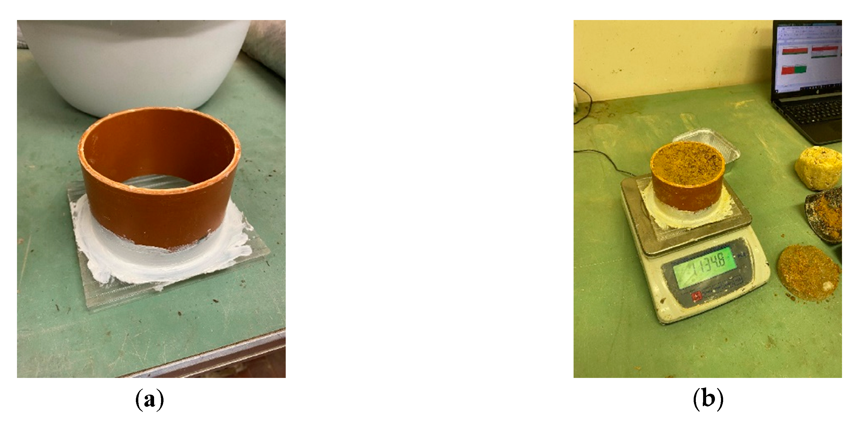
- A portion of soil is placed in a container (Figure 7a) with known mass (Tare) and internal volume (V);
- (2)
- The soil and container are weighed (Figure 7b) so that the wet sample density can be calculated by Equation (2), where is the difference between the mass of the wet soil and container assembly, and the Tare.
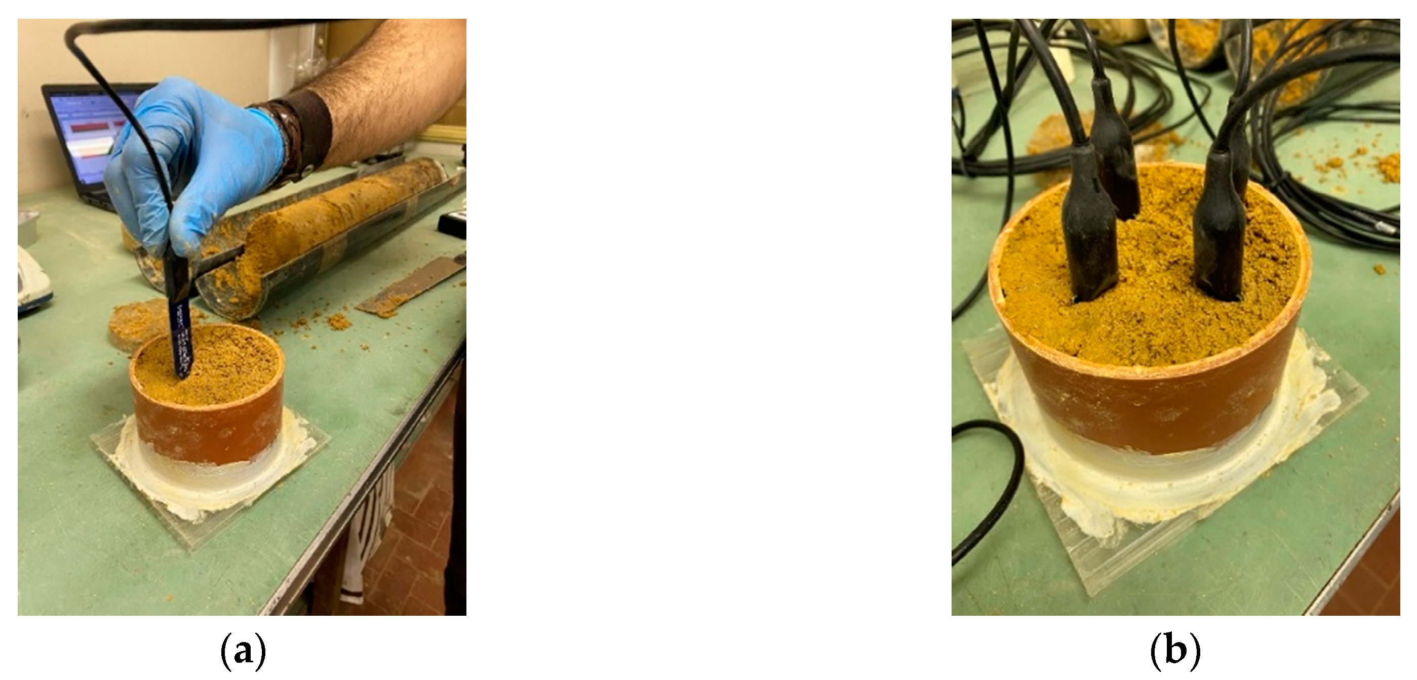
- (3)
- Four WaterScouts are inserted into the sample (Figure 8), and the raw data of the soil water content are collected from each sensor by the FieldScout Soil Sensor Reader.
- (4)
- A portion of the sample is then taken for the measurement of the gravimetric water content , which allows the dry mass of the sample to be determined with Equation (3); the apparent soil density is determined by Equation (4).
This procedure makes it possible to calculate, by means of Equation (1), the volumetric water content of a specific sample and to record the raw data associated with it, as the averages of the four output data of the sensors used in Step 3. The repetition of the above steps on soil samples with different moistures produces a series of data useful for determining the correlation between the raw data and soil moisture content.
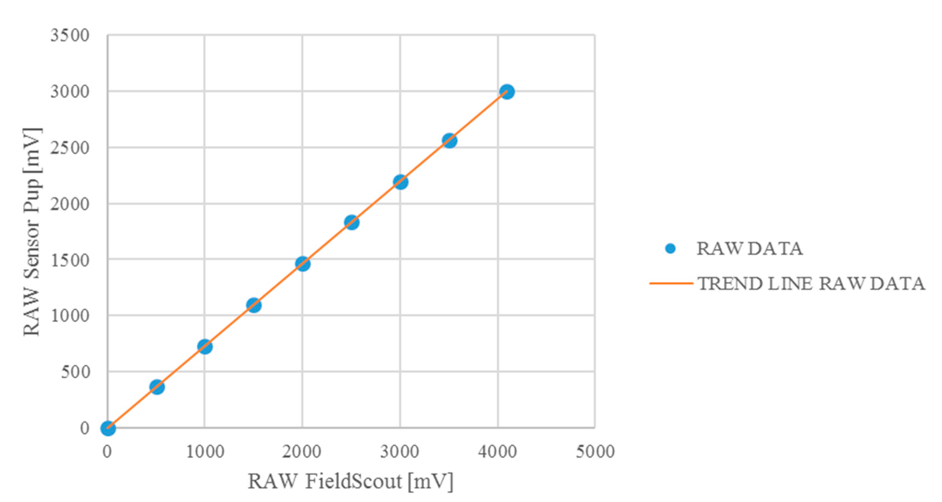
It is appropriate, however, to highlight some fundamental aspects related to the nature of the raw data or the output voltage Vout of the sensors. First, it varies depending on the supply voltage Vin of the sensors, which ranges from 3 to 5 V, and the device one decides to connect to the instrument. In fact, while the Sensor Pup supplies the sensors with an input voltage of about 3 V, the FieldScout Soil Sensor Reader supplies the sensors with that of about 5 V; consequently, the output voltages measured by the two devices are different.
Nevertheless, through an analysis of the A/D converters of the devices, it was possible to define the relationship between the two raw data.
Please note that the actual raw data used in calibration are not the Vout readings but the Vout/Vin ratios. The statistical characteristics of Equation (5) will be discussed in Section 3.2.
2.5. Field Installation
The field installation of the monitoring network starts with an inspection aimed at choosing the points at which to place the sensors and the devices necessary for transmission and reception. The Retriever must be able to pick up the radio signals of the Sensor Pups distributed in the area, and the Modem linked to it must connect to a GSM operator that ensures reliable network coverage. Therefore, the choice of the node locations necessarily depends both on the presence of a small area in which the sensors can be inserted and on the radio signal cover; the latter can be evaluated by connecting the Retriever to a PC via a USB cable and using the appropriate Retriever/Pups interface.
With reference to each measuring node, the sensors are installed in the ground at different depths in order to describe the vertical moisture profile in the upper 90 cm.
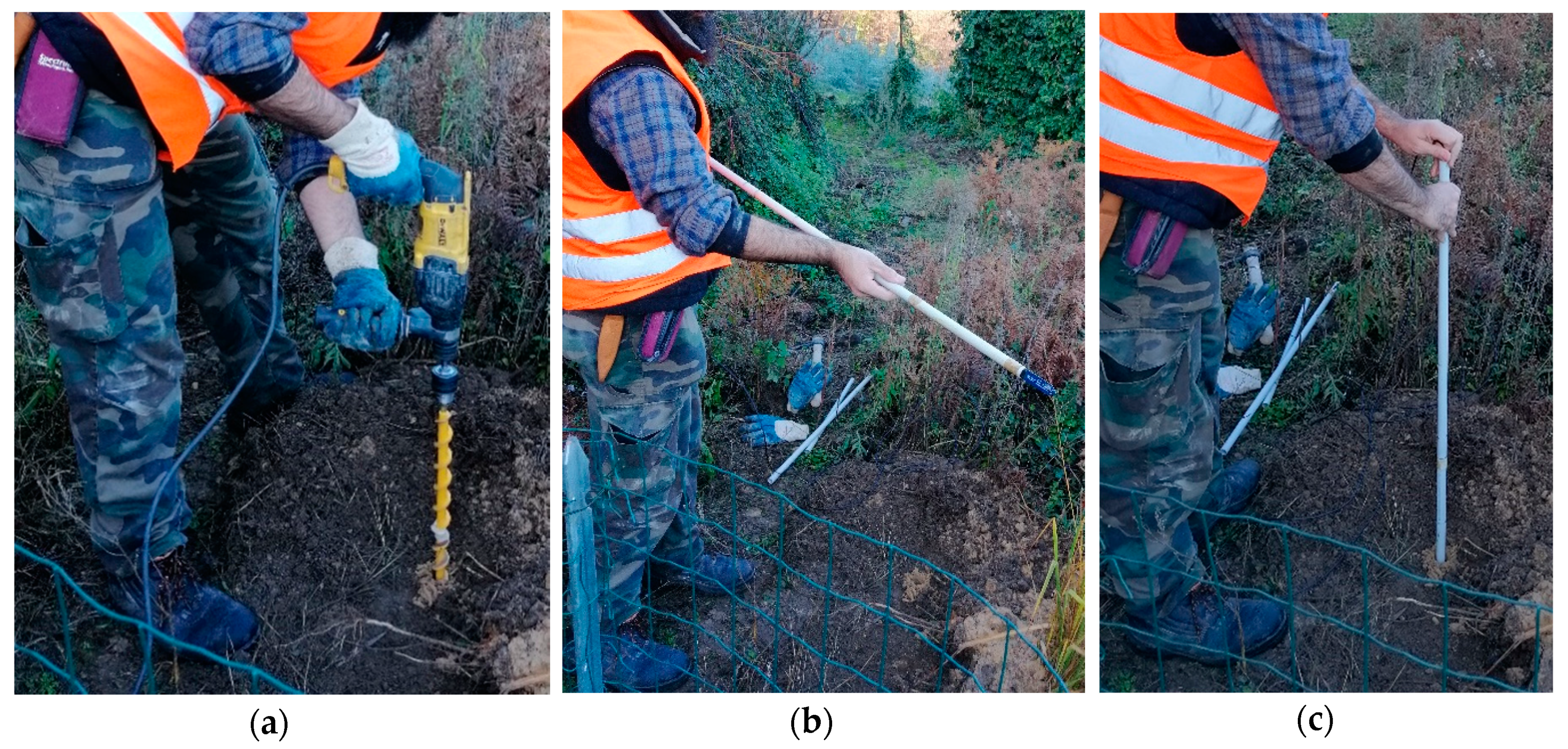
There are two main modes of installation. The fastest one involves inserting each sensor vertically at the desired depth through a pre-installation hole (Figure 9). If this operation is hampered by the presence of stones/pebbles or by meeting a particularly compact soil level, it is necessary to opt for horizontal installation from a trench front (Figure 10).
For the insertion of the WaterScouts in the ground, a PVC pipe is used; the sensor is pushed into the soil along the full probe length, being inserted at the pipe end opening, while its wire exits from the other side; the pipe is then removed when the sensor is properly set.
Whichever installation method is chosen, the sensor surfaces must be in full contact with the soil. Sometimes (especially if the soil to be penetrated by the sensor is particularly stiff), the cuttings, coming out during the drilling phase, are applied directly on the surface of the instrument, which is then simply inserted at the bottom of the pre-drilled hole without pushing, in order to avoid the rupture of the sensor. The functionality of any installed sensor must always be immediately checked, by using the FieldScout Soil Sensor Reader.
The vertical installation involves, after the positioning of the sensors, the application of a certain quantity of dry bentonite in the upper part of the drilled hole, then moistened by pouring water from the top, to seal the installation hole to avoid preferential infiltration paths for the surface runoff water.
Horizontal installation requires the insertion of the WaterScouts in horizontal pre-holes a few centimetres deep. In this case, it is not necessary to use bentonite. Despite this, the opening of a temporary excavation is needed, and once installation is complete, the subsequent backfilling alters the initial conditions with reference to water circulation. Therefore, before backfilling, it is necessary to apply a waterproof sheet on the excavation front where the sensors have been installed.
As mentioned, the Sensor Pups distributed in the area are powered by 5 V solar panels, while the Modem is connected to the power net with a transformer, although it is also possible to power it with a solar panel. The Retriever is powered by the Modem itself, through the same AUX cable used for the data transmission.
The monitoring devices are installed in a natural environment. Therefore, it is advisable to use protective sheaths coated with corrugated aluminium to prevent wild rodents from damaging the sensor cables. It is also advisable to complete the installation of the Sensor Pups and attached sensors with the construction of a small protective fence that locally surrounds the control unit support pole.
The described measuring instruments do not conflict with other monitoring devices in field, such as the GNSS used to acquire the surface displacements.
2.6. Case Studies
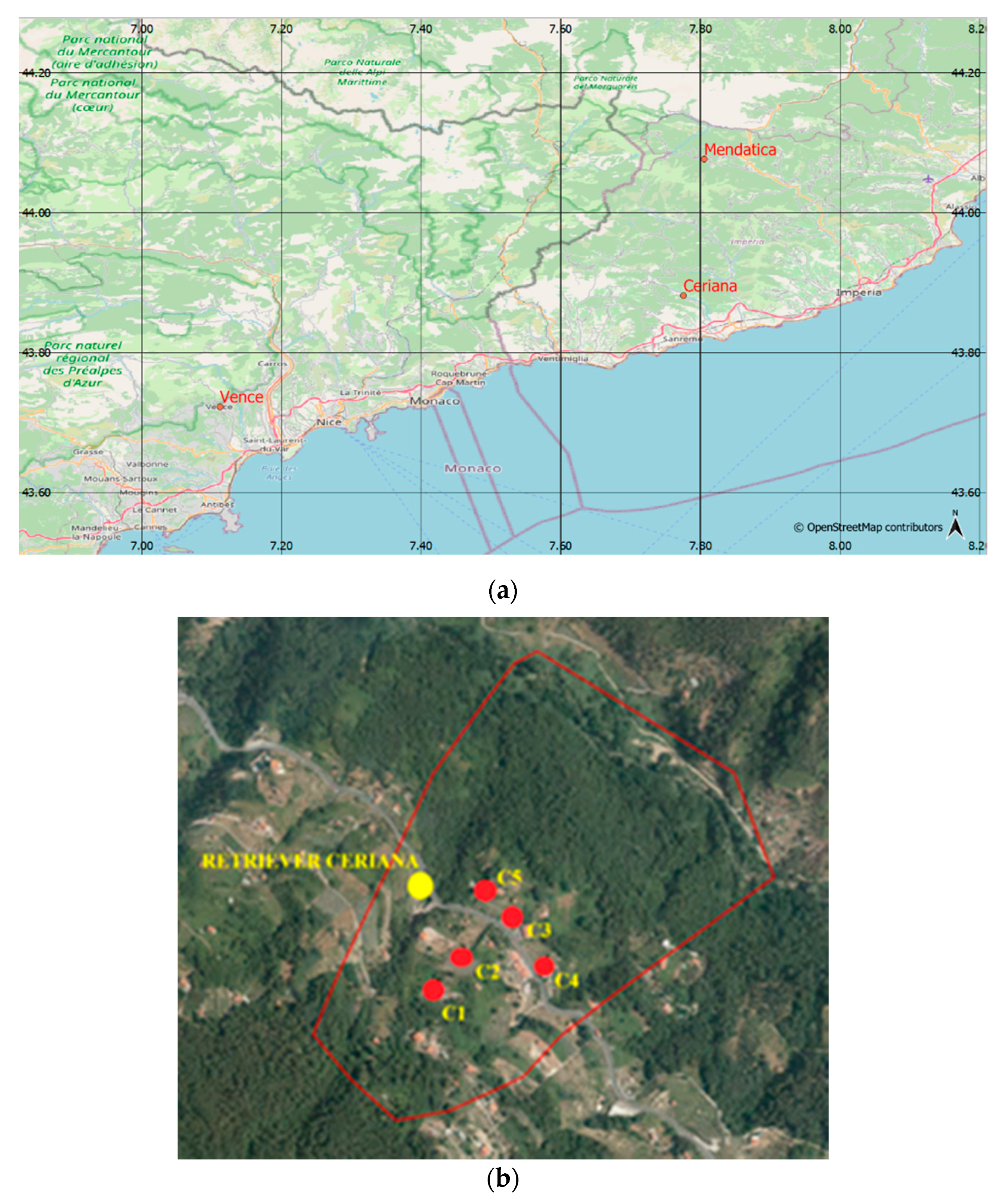
In July 2019, the inspections to decide the monitoring network nodes on the AD-VITAM project sites began (Figure 11a). Between November and December 2019, the monitoring networks at Mendatica and Ceriana-Mainardo (Figure 11b) (Italy) were completed, while the installation in Vence (France) was concluded in February 2020.
To establish the positions of the nodes, all the Sensor Pups (five for each landslide site) were activated so as to enhance the radio signal, determined by the “bridge” effect between the different control units distributed over the area. The instruments were provisionally fixed on telescopic support poles, which were placed in the planned points for ascertaining the connection between the nodes. Furthermore, it was necessary to find a suitable point for the positioning of the Retriever. Although the installation points can be chosen in advance through analysing the cartography of the territory, it is not wise to forgo a field evaluation. In fact, the nodes must be positioned so as to allow good data transmission. Once the location of the nodes was established, how to install the WaterScout sensors according to the soil properties was decided.
The deposits found in Mendatica showed the presence of boulders and particularly dense soil layers, which have repeatedly hindered the insertion of the sensors at the provided depths. Hence, at two of the five installation points, it was necessary to carry out horizontal insertion. On the contrary, the Ceriana site presented favourable installation conditions, with the exception of a single point, where the soil layers below 70 cm became very stiff, such that one of the sensors broke. The realization of the pre-holes for the installation of the WaterScouts is also useful for determining if sampling near the node will be simple. Finally, the Vence site in France (Figure 11a) presented favourable installation conditions. However, even though the deposits did not show a marked presence of boulders, the soil density was such as to contrast the sensor insertion. For this reason, it was decided to apply the soil cuttings directly on the sensor surfaces, as described above; the sensors were then vertically placed at the desired depth.
In the following, there will be exclusive reference to the results from the measurement node named C5 located in Ceriana, as the pertinent calibration of the WaterScouts had already been carried out. The soil water content measurements at node C5 (Figure 11b) will be linked to four rainfall events that occurred between May and June 2020.
3. Results
The following results are related to the behaviour of moisture sensors with the rainfall-induced changes in soil water content in the test-field scenario, described in Section 2.3. The results useful for the definition of Equation (5) are also described. Finally, some evaluations are reported of the characterization of the soil taken from one of the measurement nodes of the Ceriana-Mainardo site, as well as the results of the calibration described in Section 2.4 applied to it. Again, referring to the abovementioned node C5, the first water content measurements obtained through the described monitoring systems are then presented.
3.1. Results of the Preliminary Study on the Test-Field: Comparison between WaterScout SM100 and Drill&Drop Probe
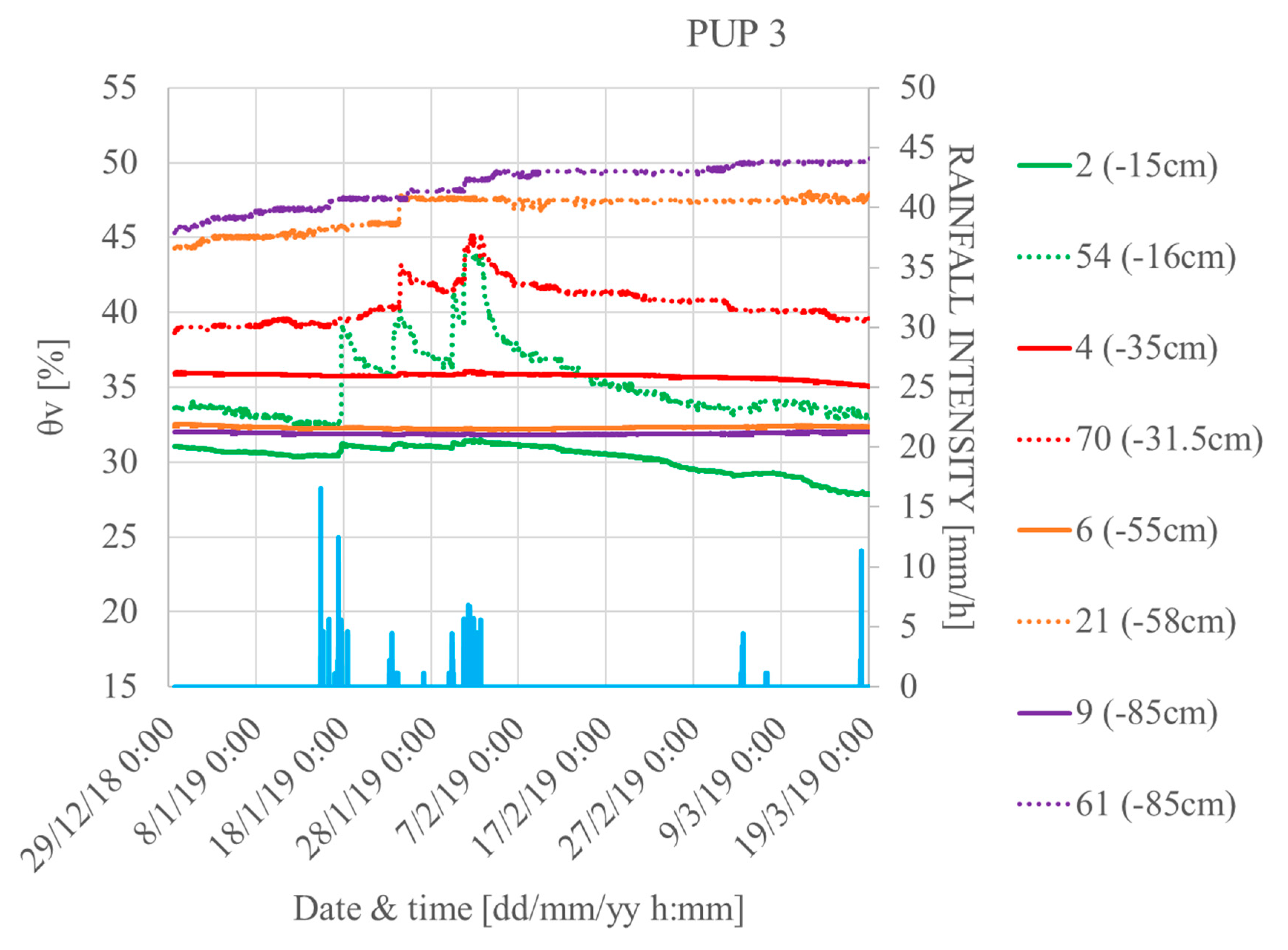
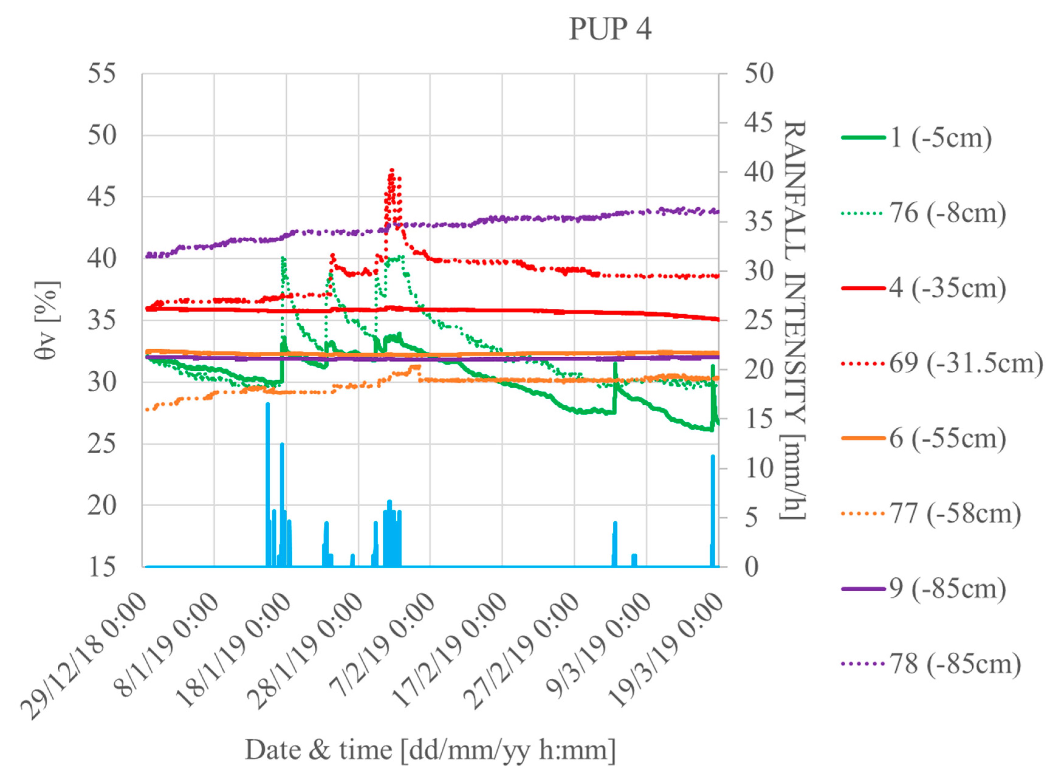
The graphs in Figure 12 and Figure 13 compare the soil water content measurements made by the sensors during the rainfalls that occurred between 29 December 2018 and 19 March 2019 at the test field. It is worth recalling that the test field was characterized by a very shallow soil layer up to a depth of 30 cm (sparsely vegetated with grass) and extremely heterogeneous and heterometric landfill material (containing stones, parts of bricks and small concrete debris) below.
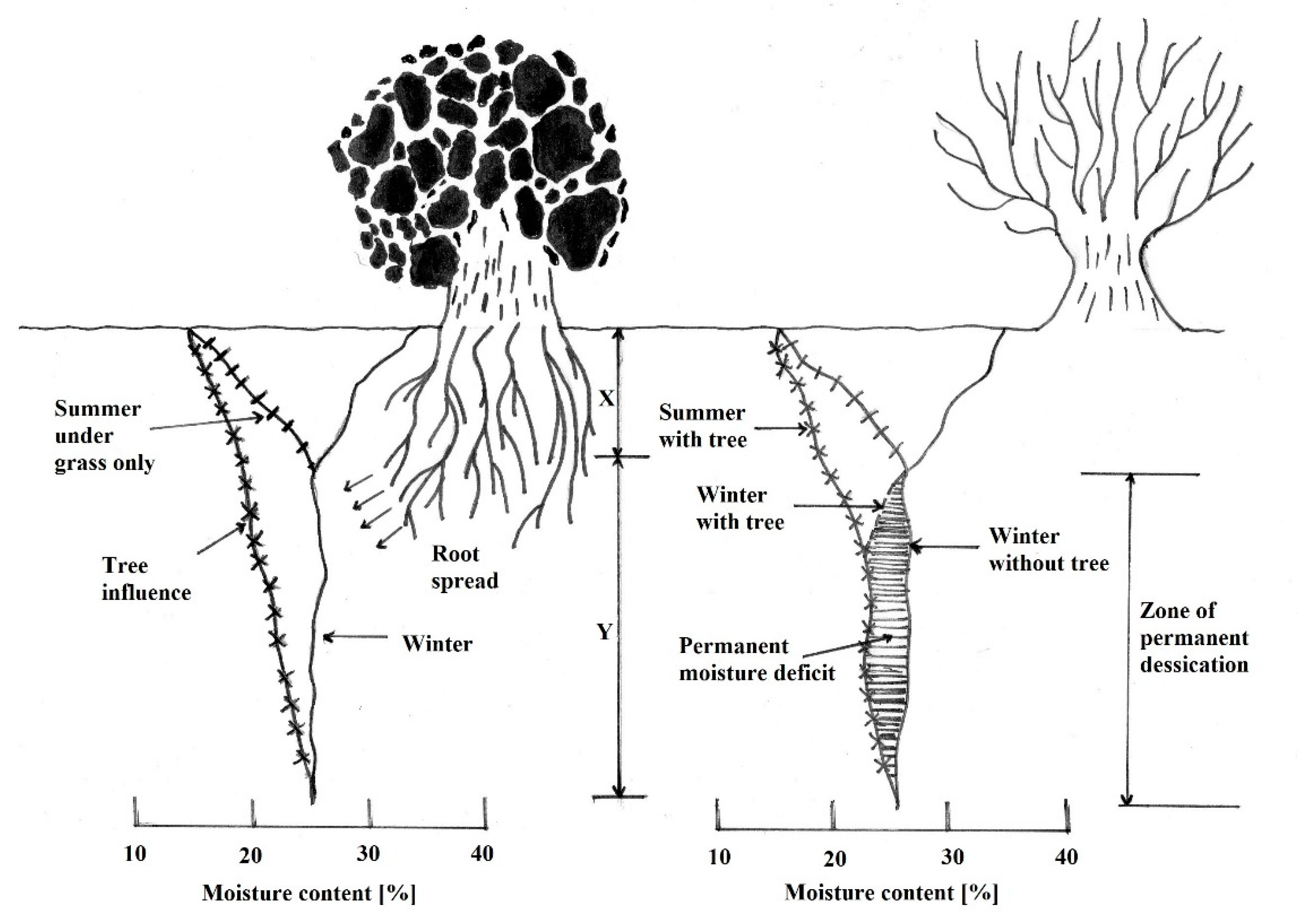
At first glance, the measurements obtained through the WaterScouts appeared to be significantly different from the moisture detected by the Drill&Drop probe, both in terms of the measured values and in terms of their variations. Drift of the signal was particularly evident at depths between 55 and 85 cm, where the soil was not significantly affected by water infiltration and evapotranspiration phenomena. Figure 14 (in accordance to [41]) shows the presence of a zone of almost constant moisture in relatively deep layers of soil and a relatively shallow zone, where a cyclic variation of moisture contents occurs. The profiles shown in Figure 14 are merely qualitative. In fact, the soil moisture profiles are influenced by the specific conditions of the site; they depend on many factors, including the characteristics and texture of the soil, the vegetation and the climate.
Figure 12 and Figure 13 show a substantial difference between the data measured by the two probes under examination. The response of the Drill&Drop sensors is quite flat, and this would have deserved further investigation. On the other hand, the measurements of the WaterScouts were not calibrated by a soil-specific law, suggesting the need to focus subsequent research on the laboratory calibration of the WaterScouts.
The measurements in the test field also indicate that close attention should be paid to the installation of sensors. Therefore, even greater care was dedicated to the subsequent installation of the sensors on site. In fact, correct installation and good soil–sensor contact are extremely important.
Since the WaterScouts are used in the monitoring networks, attention was focused on these probes, as shown in the following.
3.2. Results of the Study about the Relationship between the FieldScout Soil Sensor Reader and Sensor Pup Raw Data
Equation (5) is the result of a specific analysis of the FieldScout Soil Sensor Reader used during the calibration and installation phases. This analysis shows that the power voltage supplied by the instrument is a little more than 4 V and slightly lower than the maximum supply voltage of 5 V specified in the user manuals. Considering, therefore, the supply voltage of the Sensor Pup being equal to 3 V and 12-bit A/D conversion, Table 3 and Figure 15 show the relationship between the two raw data expressed by Equation (5), which perfectly fits the data with a coefficient of correlation R2 = 1. This approach led to a very precise relationship between the Sensor Pup and FieldScout raw data.
3.3. Results of the Characterization of the Soil Sampled in Ceriana-Mainardo for the Calibration Procedure
The described calibration operations were performed on the soil pertinent to a borehole realized at the node, called C5, of the monitoring network in Ceriana-Mainardo (Imperia, Italy). The landslide deposit is composed of heterogeneous and heterometric material.
The core samples, retrieved from the upper 60 cm of the soil, did not show substantial variability with depth. The calibration of the soil moisture sensors confirmed this observation. Therefore, it was decided to report the properties of a single portion of the extracted soil, representative of the material between 35.5 cm and 45.5 cm depth below ground level (Figure 16). This portion was extracted from the core sample, limiting the disturbance in order to evaluate the porosity n, the voids index e and, therefore, the relative density Dr (Table 4).
3.4. Calibration Results for the Soil Sample Taken from Ceriana-Mainardo
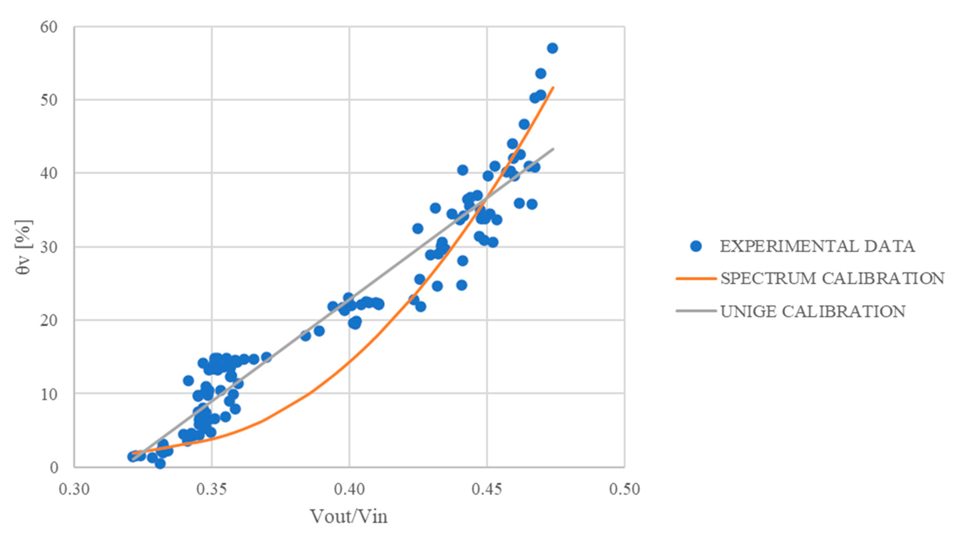
The first results of the calibration procedure for the soil at the node C5 in Ceriana-Mainardo (IM) are shown in Figure 17. By interpolating the data by linear regression, it is possible to obtain the calibration correlation shown in Table 5. Figure 17 also shows the comparison between the calibration function exposed in Table 5 and the relationship provided by Spectrum Tec., which is not linear. The validity range for the calibration function (named UNIGE CALIBRATION in Figure 17) expressed in Table 6 is .
Although the experimental data (Figure 17) suggest that two trends can be identified, a single calibration equation is introduced in the interest of simplicity, which represents the overall trend of the data. In fact, upon analysing other possible calibration laws (e.g., a segmented linear regression and second-degree polynomial curve), the results did not show any significant improvement compared to the simple trend line indicated in Table 5.
3.5. Rain Data and Water Content Measurements in Ceriana-Mainardo
In November 2000, Ceriana-Mainardo was subject to shallow instabilities, which particularly involved the Provincial Road n. 44 and the adjacent areas (Figure 18a). Geognostic investigations (continuous core drillings) and geotechnical and geophysical surveys were carried out. Laboratory soil characterizations, light dynamic penetrations (type Penny30), inclinometers and geophysical tests (seismic refraction alignments and down-holes), allowed the characterization of the subsoil sequences. Monitoring the site with piezometers and rain gauges made it possible to assess the water table fluctuations and occurring rainfalls, respectively.
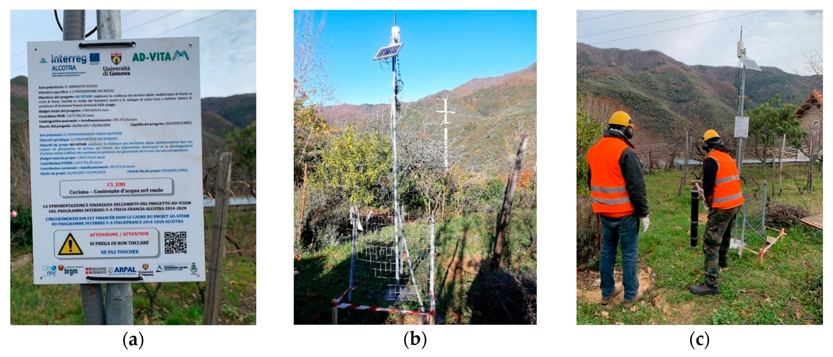
The soil moisture monitoring network installed at the Ceriana-Mainardo site has been in operation since December 2019. At the WSN nodes, distributed as shown in Figure 18b, soil water content values are recorded every 5 min. Four measuring points were installed at each node. At node C5 (represented in Figure 11b), the sensors are placed at 10 cm, 35 cm, 55 cm and 85 cm below ground level. The sensors are similarly located in the other four nodes. All the sensors in Ceriana-Mainardo were installed vertically. Node C5 is shown in Figure 19a,b.
In Ceriana-Mainardo, two core samples were taken (similarly to how samples were taken in Mendatica and Vence). They were adjacent to each of the measuring nodes; only one sampler was broken on site. Figure 19c shows the sampling at node C5.
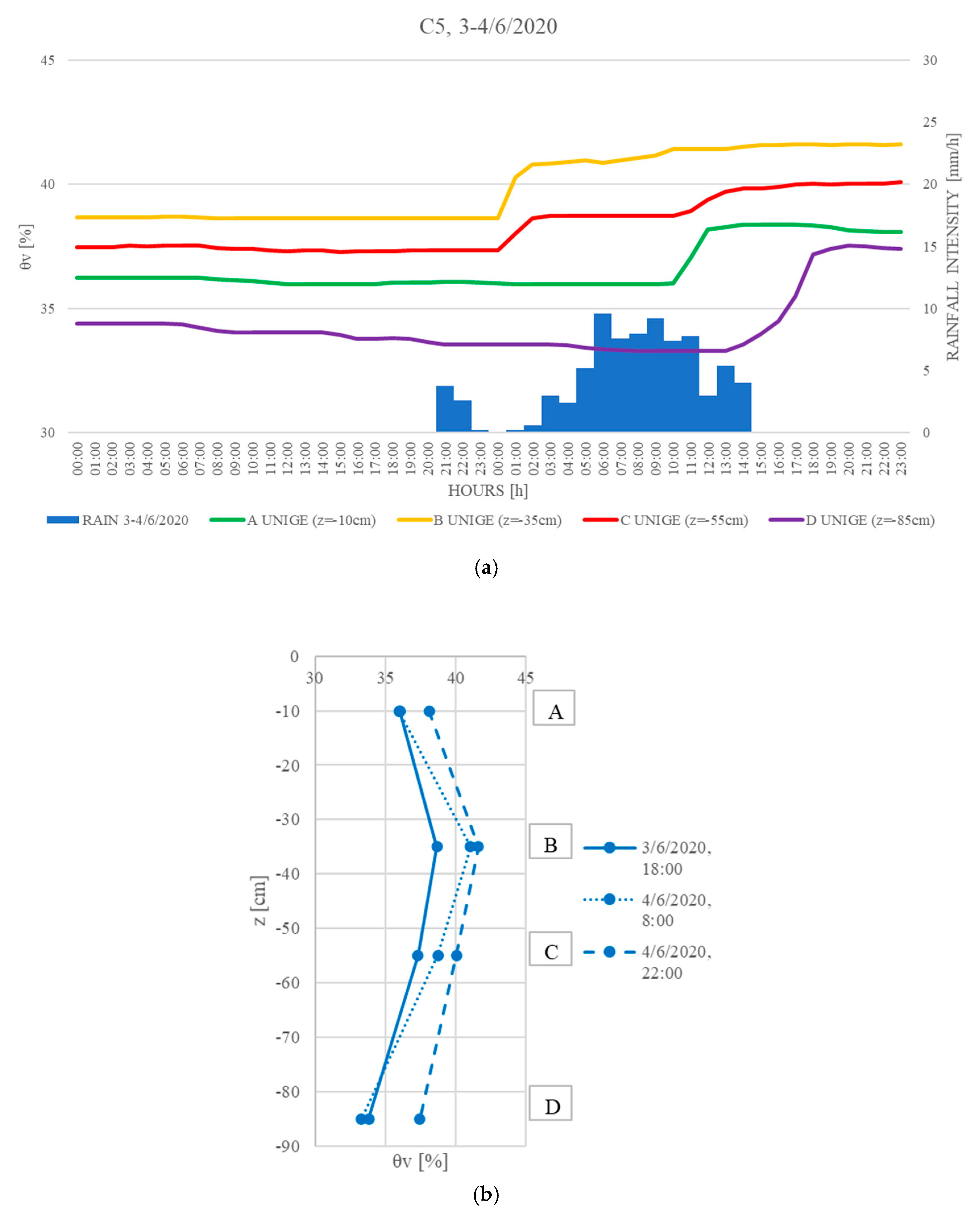
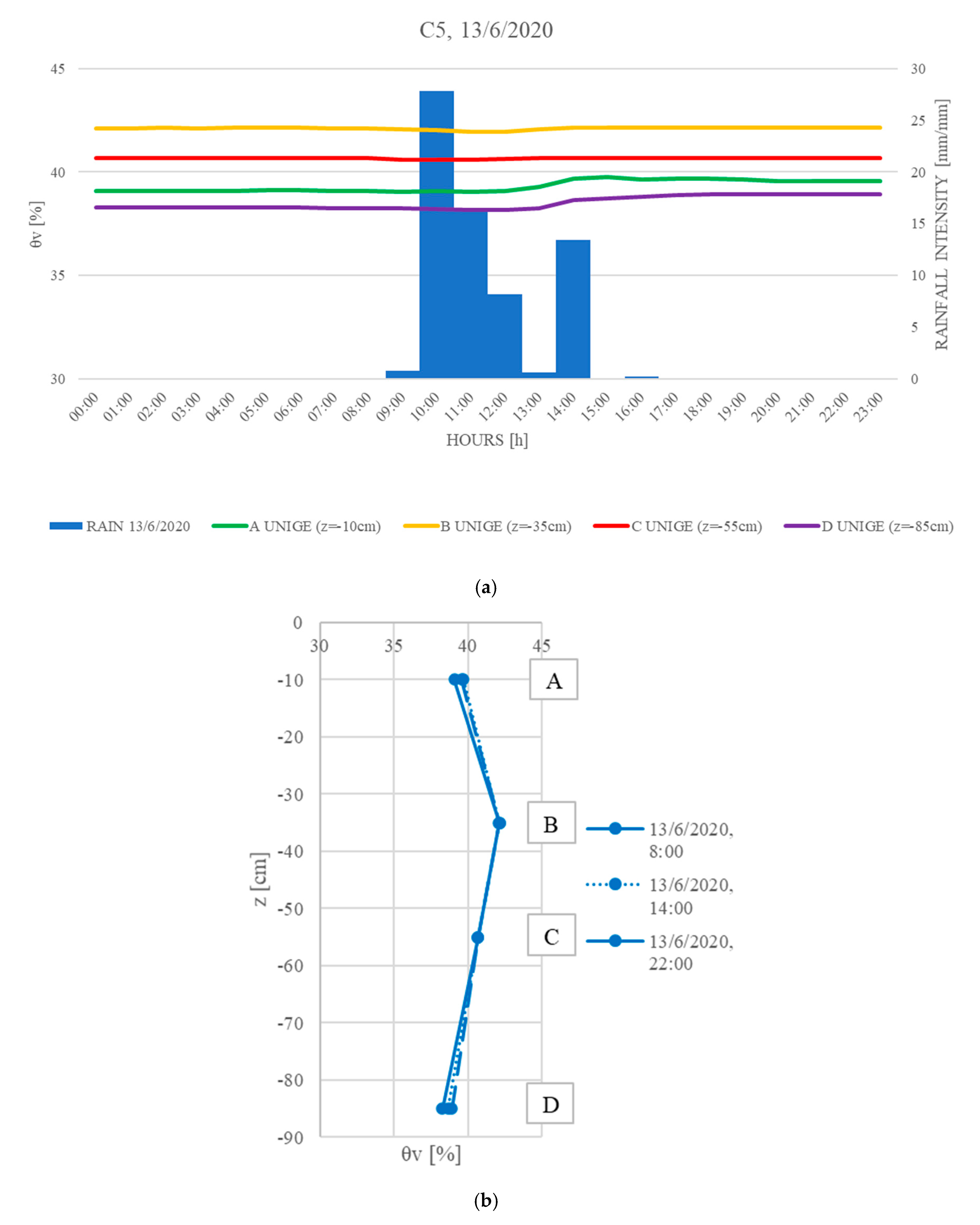
The measurements of the water content in the soil at node C5 during some rainfall events (Table 6, Table 7 and Table 8) are presented below; at C5, the steady water table fluctuates around 21 m below ground level. Figure 20a, Figure 21a and Figure 22a show the trends in water content measured at various depths. The represented soil moisture values were calibrated by the regression law indicated in Table 5 denoted by the acronym UNIGE. The graphs allow the understanding of how the water content varies over time at the four depths where the sensors are positioned. The rainfalls that occurred are also represented.
Figure 20b,c, Figure 21b and Figure 22b show the variations of the vertical moisture profiles obtained by the UNIGE calibration law. Three profiles are represented; they are referred to three time-windows: before the beginning of the rainfall (undisturbed conditions), immediately after the rainfall peak, and at the end of the event.
4. Discussion
The water content measurements reported in this paper were taken at a single node of one of the five sites studied in the AD-VITAM project (the C5 at Ceriana-Mainardo). These measurements correspond to a short period, since the monitoring network was installed a few months ago.
The measurements were suitably calibrated because of the experiments performed on the soil taken on site at this node.
The data obtained by the field measurements are encouraging. In fact, Figure 20a, Figure 21a and Figure 22a not only show good behaviour for the sensors, which continuously detect variations in soil moisture, but also indicate that no preferential infiltration paths were generated during the installation phases. In fact, as shown in those figures, the increases in water content do not occur immediately after the rainfall but are recorded a few hours after the rain peaks. Figure 20b,c, Figure 21b and Figure 22b clearly show the changes in water content at shallow depths when rainfall occurs. Thus, the measurements over time and soil water content profiles seem to capture the soil moisture dynamics, demonstrating their usefulness for describing the slope response to rainfalls.
Full analysis will be possible when water content measurements become available at all nodes and when the database becomes sufficiently rich and representative. All five sites will be equipped with the LAMP system by the end of 2020. This will allow the study of the response of the slopes to the rainfalls, both in real time (thanks to the WSN) and for prediction (if the short-term forecasted rains are considered), as well as improving landslide risk management, the design of mitigation measures and territorial planning [42].
5. Conclusions
The LAMP system was formulated for the analysis and forecasting of susceptibility to landslides triggered by rainfalls. It is based on an integrated hydrological–geotechnical model that is physically based and fed by a low-cost, self-sufficient, remotely manageable and easily replaceable/relocatable monitoring network. WaterScout capacitive sensors are positioned at sites potentially susceptible to landslides, at shallow depths (typically less than 1 m).
Knowledge of the near-surface water content over time is needed for hydrological and geotechnical analysis, the study of the hydro-mechanical contribution from the vegetation and, eventually, landslide risk mitigation with soil bio-engineering countermeasures. Additionally, the monitoring of the soil water content may be useful for analysing the soil moisture conditions immediately after emergencies, to determine when the risk conditions no longer exist.
This paper describes the installation phases for the monitoring networks, pinpointing the care needed in the choice of nodes, the arrangement of the sensors and, not least, the protection of the materials left on site. Particular attention has been paid to experiments conducted to evaluate the reliability of the used sensors and calibrate them. Soil-specific calibration was carried out in the laboratory on soil samples taken very near to the WSN instrumented verticals.
WaterScout calibration is very important. The WaterScout-SM100’s operating frequency range is 70–80 MHz, and relevant variations in the sensor response may occur, especially in clayey soils. A soil-specific calibration is particularly recommended, to take into account the characteristics and textures of the in situ soil.
Although most soil moisture sensors are sensitive to temperature and salinity, the WaterScouts are little affected by these factors [3], so they can be adopted for effective environmental monitoring.
Since these probes must be inserted into the soil and be in contact with it, their use is possible in soils that can be penetrated, and the immediate confirmation of full soil–sensor contact with a FieldScout Soil Sensor Reader is recommended. In fact, such a reading allows the operator to immediately determine if the sensor has made full contact with the soil; a measurement close to zero would indicate partial contact with the air.
These sensors, providing continuous and real-time data, are substantially low in cost, easily relocatable and replaceable. Moreover, a complete and remotely manageable soil moisture monitoring network is relatively inexpensive, does not require onerous preliminary operations and is not bulky or unsightly. A monitoring network made up of five measurement nodes can be installed by three expert operators in only 2–3 days.
The soil water content measurements, so far acquired by the recently installed monitoring networks, are very satisfying and encouraging. The integration of such monitoring system in the LAMP system may be useful for the analysis and prediction of landslides triggered by rainfalls and could be of real support in risk management.
Author Contributions
Conceptualization, R.B., B.F. and R.P.; methodology, R.B., B.F., A.I. and R.P.; software, R.B., B.F., A.I. and R.P.; validation, A.I.; formal analysis. A.I.; investigation, R.B., B.F., A.I. and R.P.; resources, R.B., B.F., A.I. and R.P.; data curation, B.F. and A.I.; writing—original draft preparation, R.B., B.F., A.I. and R.P.; writing—review and editing, R.B., B.F., A.I. and R.P.; visualization, R.B. and A.I.; supervision, R.B. and R.P.; project administration, R.B. and B.F.; funding acquisition, R.B., B.F. and R.P. All authors have read and agreed to the published version of the manuscript.
Funding
This research was funded by Interreg V-A France-Italie, ALCOTRA “AD-VITAM” 2014-2020, Axis 2, Safe Environment programme, grant number 1573. The APC was funded by Roberto Passalacqua’s research funds from the University of Genoa.
Acknowledgments
The authors acknowledge the support given by AD-VITAM Partners. A particular acknowledgement goes to the Unione dei Comuni della Valle Argentina e Armea and to the lab technicians of the Department of Civil, Chemical and Environmental Engineering of the University of Genoa.
Conflicts of Interest
The authors declare no conflict of interest. The funders had no role in the design of the study; in the collection, analyses or interpretation of data; in the writing of the manuscript; or in the decision to publish the results.
References
- Tarantino, A.; Pozzato, A. Strumenti per il monitoraggio della zona non satura. Riv. Ital. Geotec. 2008, 3, 109–125. [Google Scholar]
- Nagahage, E.A.A.D.; Nagahage, I.S.P.; Fujino, T. Calibration and Validation of a Low-Cost Capacitive Moisture Sensor to Integrate the Automated Soil Moisture Monitoring System. Agriculture 2019, 9, 141. [Google Scholar] [CrossRef] [Green Version]
- Adla, S.; Rai, N.K..; Sri Karumanchi, H.; Tripathi, S.; Disse, M.; Pande, S. Laboratory Calibration and Performance Evaluation of Low-Cost Capacitive and Very Low-Cost Resistive Soil Moisture Sensors. Sensors 2020, 20, 363. [Google Scholar] [CrossRef] [PubMed] [Green Version]
- Iverson, R.M. Landslide triggering by rain infiltration. Water Resour. Res. 2000, 36, 1897–1910. [Google Scholar] [CrossRef] [Green Version]
- Crosta, G.B.; Frattini, P. Distributed modelling of shallow landslides triggered by intense rainfall. Nat. Hazards Earth Syst. Sci. 2003, 3, 81–93. [Google Scholar] [CrossRef] [Green Version]
- Vassallo, R.; Mancuso, C.; Vinale, F. Effects of net stress and suction history on the small strain stiffness of a compacted clayey silt. Can. Geotech. J. 2007, 44, 447–462. [Google Scholar] [CrossRef]
- Mancuso, C.; Vassallo, R.; d’Onofrio, A. Small strain behavior of a silty sand in controlled-suction resonant column - Torsional shear tests. Can. Geotech. J. 2011, 39, 22–31. [Google Scholar] [CrossRef]
- Mazzuoli, M.; Bovolenta, R.; Berardi, R. Experimental Investigation on the Mechanical Contribution of Roots to the Shear Strength of a Sandy Soil. Proced. Eng. 2016, 158, 45–50. [Google Scholar] [CrossRef] [Green Version]
- Bordoni, M.; Meisina, C.; Vercesi, A.; Bischetti, G.B.; Chiaradia, E.A.; Vergani, C.; Chersich, S.; Valentino, R.; Bittelli, M.; Comolli, R.; et al. Quantifying the contribution of grapevine roots to soil mechanical reinforcement in an area susceptible to shallow landslides. Soil Tillage Res. 2016, 163, 195–206. [Google Scholar] [CrossRef]
- Bovolenta, R.; Mazzuoli, M.; Berardi, R. Soil bio-engineering techniques to protect slopes and prevent shallow landslides. Riv. Ital. Geotec. 2018, 52, 44–65. [Google Scholar]
- Balzano, B.; Tarantino, A.; Ridley, A. Preliminary analysis on the impacts of the rhizosphere on occurrence of rainfall-induced shallow landslides. Landslides 2019, 16, 1885–1901. [Google Scholar]
- Bittelli, M.; Valentino, R.; Salvatorelli, F.; Rossi Pisa, P. Monitoring soil-water and displacement conditions leading to landslide occurrence in partially saturated clays. Geomorphology 2012, 173, 161–173. [Google Scholar] [CrossRef]
- Comegna, L.; Damiano, E.; Greco, R.; Guida, A.; Olivares, L.; Picarelli, L. Field hydrological monitoring of a sloping shallow pyroclastic deposit. Can. Geotech. J. 2016, 53, 1125–1137. [Google Scholar] [CrossRef] [Green Version]
- Bordoni, M.; Valentino, R.; Meisina, C.; Bittelli, M.; Chersich, S. A simplified approach to assess the soil saturation degree and stability of a representative slope affected by shallow landslides in Oltrepò Pavese (Italy). Geosciences 2018, 8, 472. [Google Scholar] [CrossRef] [Green Version]
- Bovolenta, R.; Passalacqua, R.; Federici, B.; Sguerso, D. Monitoring of Rain-Induced Landslides for the Territory Protection: The AD-VITAM Project. Lect. Notes Civ. Eng. 2020, 40, 138–147. [Google Scholar]
- Bovolenta, R.; Passalacqua, R.; Federici, B.; Sguerso, D. LAMP-LAndslide Monitoring and Predicting for the analysis of landslide susceptibility triggered by rainfall events. In Landslides and Engineered Slopes. Experience, Theory and Practice, Proceedings of the 12th International Symposium on Landslides, Napoli, Italy, 12–19 June 2016; CRC Press, Taylor & Francis Group: London, UK, 2016; Volume 1, pp. 517–522. [Google Scholar]
- Passalacqua, R.; Bovolenta, R.; Federici, B.; Balestrero, D. A physical model to assess landslide susceptibility on large areas: recent developments and next improvements. Proced. Eng. 2016, 158, 487–492. [Google Scholar] [CrossRef] [Green Version]
- Passalacqua, R.; Bovolenta, R.; Federici, B. An integrated hydrological-geotechnical model in GIS for the analysis and prediction of large-scale landslides triggered by rainfall events. In Engineering Geology for Society and Territory: Landslide Processes; Springer: Berlin, Germany, 2015; Volume 2, pp. 1799–1803. [Google Scholar]
- Passalacqua, R.; Bovolenta, R.; Spallarossa, D.; De Ferrari, R. Geophysical site characterization for a large landslide 3-D modelling. In Geotechnical and Geophysical Site Characterization 4-Proceedings of the 4th International Conference on Site Characterization 4, ISC-4; CRC Press, Taylor & Francis Group: London, UK, 2013; Volume 1, pp. 1765–1771. [Google Scholar]
- Federici, B.; Bovolenta, R.; Passalacqua, R. From rainfall to slope instability: an automatic GIS procedure for susceptibility analyses over wide areas. Geomat. Nat. Hazards Risk 2015, 6, 454–472. [Google Scholar] [CrossRef]
- Hydrology, National Engineering Handbook, Supplement A, Section 4, Chapter 10; USDA: Washington, DC, USA, 1956.
- Bordoni, M.; Bittelli, M.; Valentino, R.; Chersich, S.; Persichillo, M.G.; Meisina, C. Soil Water Content Estimated by Support Vector Machine for the Assessment of Shallow Landslides Triggering: The Role of Antecedent Meteorological Conditions. Environ. Model. Assess. 2018, 23, 333–352. [Google Scholar] [CrossRef]
- Coppola, L.; Reder, A.; Rianna, G.; Pagano, L. The Role of Cover Thickness in the Rainfall-Induced Landslides of Nocera Inferiore 2005. Geosciences 2020, 10, 228. [Google Scholar] [CrossRef]
- Skempton, A.W.; DeLory, F.A. Stability of natural slopes in London Clay. In Proceedings of the 4th International Conference on Soil Mechanics and Foundation Engineering; Butterworths: London, UK, 1957; Volume 2, pp. 378–381. [Google Scholar]
- Alvioli, M.; Baum, R.L. Parallelization of the TRIGRS model for rainfall-induced landslides using the message passing interface. Environ. Model. Softw. 2016, 81, 122–135. [Google Scholar] [CrossRef]
- Baum, R.L.; Savage, W.Z.; Godt, J.W. TRIGRS-A Fortran Program for Transient Rainfall Infiltration and Grid-Based Regional Slope-Stability Analysis: Open-File Report 02-424; U.S. Geological Survey: Reston, VA, USA, 2002; p. 38. [Google Scholar]
- Baum, R.L.; Savage, W.Z.; Godt, J.W. TRIGRS-A Fortran Program for Transient Rainfall Infiltration and Grid-Based Regional Slope-Stability Analysis, Version 2.0: Open-File Report 2008-1159; U.S. Geological Survey: Reston, VA, USA, 2008. [Google Scholar]
- Montrasio, L.; Valentino, R. A model for triggering mechanisms of shallow landslides. Nat. Hazards Earth Syst. Sci. 2008, 8, 1149–1159. [Google Scholar]
- Passalacqua, R.; Bovolenta, R. Landslides’ susceptibility on large surfaces triggered by rain histories. In Geotechnical Engineering for Infrastructure and Development, Proceedings of the XVI European Conference on Soil Mechanics and Geotechnical Engineering, Edinburgh, UK, 13–17 September 2015; British Geotechnical Association: London, UK, 2015; Volume 4, pp. 1831–1836. [Google Scholar]
- Chirico, G.B.; Borga, M.; Tarolli, P.; Rigon, R.; Preti, F. Role of vegetation on slope stability under transient unsaturated conditions. Proced. Environ. Sci. 2013, 19, 932–941. [Google Scholar] [CrossRef]
- Sguerso, D.; Labbouz, L.; Walpersdorf, A. 14 years of GPS tropospheric delays in the French–Italian border region: comparisons and first application in a case study. Appl. Geomat. 2015, 8, 1–13. [Google Scholar] [CrossRef]
- Ferrando, I.; Federici, B.; Sguerso, D. 2D PWV monitoring of a wide and orographically complex area with a low dense GNSS network. Earth Planets Space 2018, 70, 1–21. [Google Scholar] [CrossRef]
- Bishop, A.W. The principle of effective stress. Tek. Ukebl. 1959, 106, 859–863. [Google Scholar]
- Fredlund, D.G.; Morgenstern, N.R.; Widger, R.A. The shear strength of unsaturated soils. Can. Geotech. J. 1978, 15, 313–321. [Google Scholar] [CrossRef]
- Lu, N.; Godt, J. Infinite slope stability under steady unsaturated seepage conditions. Water Resour. Res. 2008, 44, 1–13. [Google Scholar] [CrossRef]
- Campora, M.; Palla, A.; Gnecco, I.; Bovolenta, R.; Passalacqua, R. The laboratory calibration of a soil moisture capacitance probe in sandy soils. Soil Water Res. 2019, 15, 75–84. [Google Scholar] [CrossRef] [Green Version]
- Calibration Manual for Sentek Soil Moisture Sensors, Version 2.0; Sentek Sensor Technologies: Stepney, Australia, 2011.
- Retriever & Pup Wireless Network: Product Manual; Spectrum Techologies, Inc.: Thayer Court Aurora, IL, USA, 2015.
- Soil Sensor Reader: Product Manual; Spectrum Techologies, Inc.: Thayer Court Aurora, IL, USA, 2015.
- WaterScout SM100 Soil Moisture Sensor: Product Manual; Spectrum Techologies, Inc.: Thayer Court Aurora, IL, USA, 2015.
- Pineda-Jaimes, J.A.; Murillo-Feo, C.A.; Colmenares, J.E. Characterization of pavement pathologies associated with the action of plant species in a road at western Sabana de Bogota. Épsilon 2015, 25, 39–68. [Google Scholar]
- Bovolenta, R.; Federici, B.; Berardi, R.; Passalacqua, R.; Marzocchi, R.; Sguerso, D. Geomatics in support of geotechnics in landslide forecasting, analysis and slope stabilization. Geoing. Ambient. Miner. 2017, 151, 57–62. [Google Scholar]
Figure 1.
Chronological chart of the research activities.

Figure 2.
Flow chart of the IHG model.

Figure 3.
Flow chart of the monitoring network (Retriever & Pups Launch Utility: Version 1.2.7.3, Copyright 2016 Spectrum Technologies Inc., Aurora, IL, USA 60504).
Figure 3.
Flow chart of the monitoring network (Retriever & Pups Launch Utility: Version 1.2.7.3, Copyright 2016 Spectrum Technologies Inc., Aurora, IL, USA 60504).

Figure 4.
(a) The WaterScout SM100; (b) The FieldScout pocket Soil Sensor Reader.

Figure 5.
The Drill&Drop probe.

Figure 6.
(a) Details of the specifically developed lower ring with a cutting edge; (b) The components as mounted on the sampler during on-site collection.
Figure 6.
(a) Details of the specifically developed lower ring with a cutting edge; (b) The components as mounted on the sampler during on-site collection.

Figure 7.
(a) Container; (b) Weighing of the wet soil sample.

Figure 8.
(a) Insertion of the first moisture sensor into the wet sample; (b) Final arrangement of the four sensors.
Figure 8.
(a) Insertion of the first moisture sensor into the wet sample; (b) Final arrangement of the four sensors.

Figure 9.
Vertical installation: (a) Creation of the vertical hole; (b) Positioning of the WaterScout in the PVC pipe; (c) Insertion of the sensor in the hole.
Figure 9.
Vertical installation: (a) Creation of the vertical hole; (b) Positioning of the WaterScout in the PVC pipe; (c) Insertion of the sensor in the hole.

Figure 10.
Example of a horizontal installation.

Figure 11.
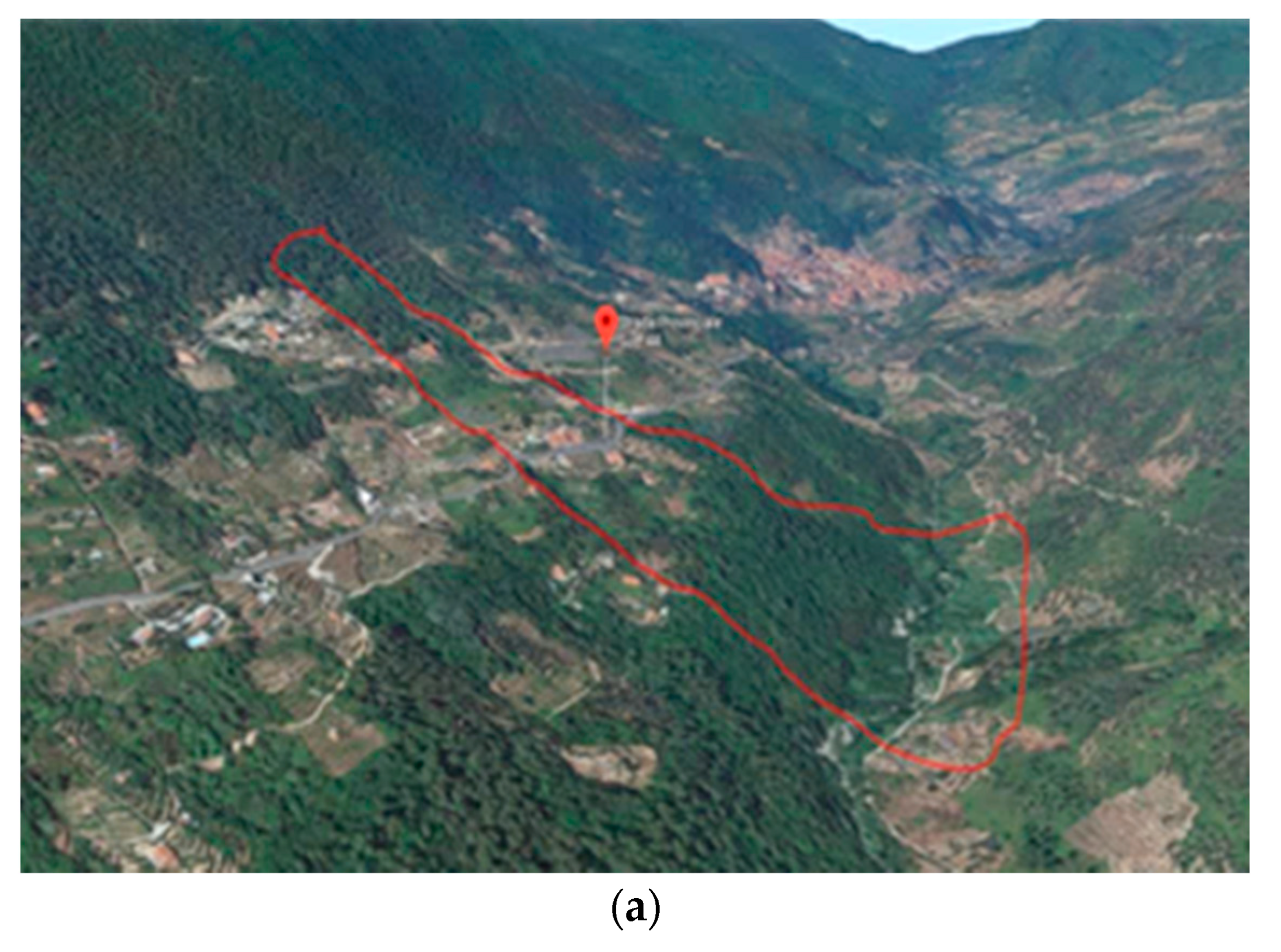
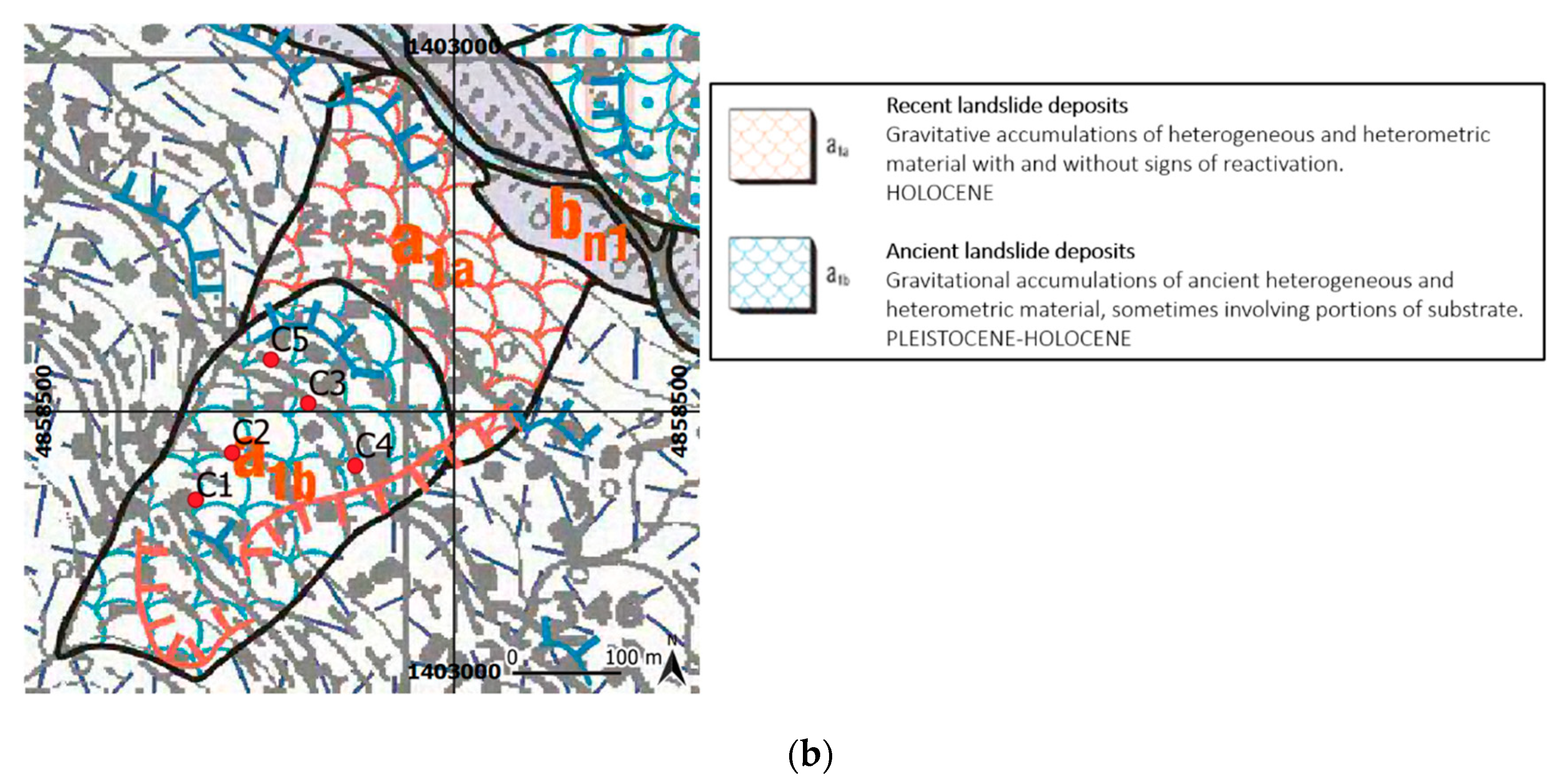
(a) Location of Ceriana, Mendatica and Vence (map in WGS84); (b) Installed monitoring network. The nodes (red dots) are denoted by C1–C5.
Figure 11.
(a) Location of Ceriana, Mendatica and Vence (map in WGS84); (b) Installed monitoring network. The nodes (red dots) are denoted by C1–C5.

Figure 12.
Measurements by WaterScout n.54, n.70, n.21 and n.61 and by the pertinent reference sensors n.2, n.4, n.6 and n.9 of Drill&Drop for 29 December 2018 to 19 March 2019.
Figure 12.
Measurements by WaterScout n.54, n.70, n.21 and n.61 and by the pertinent reference sensors n.2, n.4, n.6 and n.9 of Drill&Drop for 29 December 2018 to 19 March 2019.

Figure 13.
Measurements by WaterScout n.76, n.69, n.77 and n.78 and by the pertinent reference sensors n.1, n.4, n.6 and n.9 of Drill&Drop for 29 December 2018 to 19 March 2019.
Figure 13.
Measurements by WaterScout n.76, n.69, n.77 and n.78 and by the pertinent reference sensors n.1, n.4, n.6 and n.9 of Drill&Drop for 29 December 2018 to 19 March 2019.

Figure 14.
Changes in soil moisture content: tree influence (summer) on the left and tree influence (winter) on the right.
Figure 14.
Changes in soil moisture content: tree influence (summer) on the left and tree influence (winter) on the right.

Figure 15.
Relationship between FieldScout Soil Sensor Reader and Sensor Pup raw data.

Figure 16.
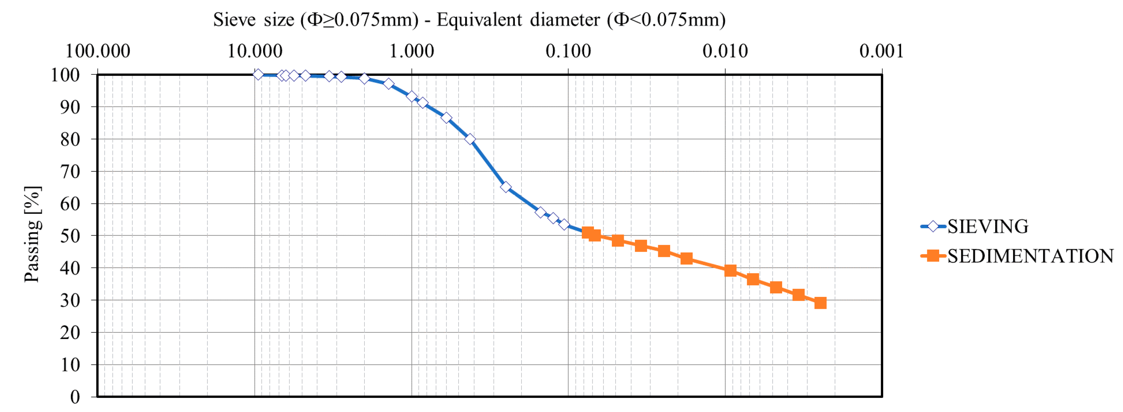
Grain size curve.

Figure 17.
Comparison between the Spectrum Tec. calibration law (SPECTRUM CALIBRATION) and the soil-specific calibration law determined by the University of Genoa (UNIGE CALIBRATION).
Figure 17.
Comparison between the Spectrum Tec. calibration law (SPECTRUM CALIBRATION) and the soil-specific calibration law determined by the University of Genoa (UNIGE CALIBRATION).

Figure 18.
Ceriana-Mainardo: (a) Landslide perimeter view overlapped in 3D; (b) Geological map. The landslide perimeter (red polyline) and the nodes C1–C5 (red dots) are reported.
Figure 18.
Ceriana-Mainardo: (a) Landslide perimeter view overlapped in 3D; (b) Geological map. The landslide perimeter (red polyline) and the nodes C1–C5 (red dots) are reported.


Figure 19.
C5 node: (a) Node identification and warning signboard; (b) Carrying and rising pole of both the Sensor Pup and the solar panel; (c) Soil sampling.
Figure 19.
C5 node: (a) Node identification and warning signboard; (b) Carrying and rising pole of both the Sensor Pup and the solar panel; (c) Soil sampling.

Figure 20.
(a) May 2020 rainfall events and soil water contents; (b) Vertical soil moisture profiles 16 May 2020; (c) Vertical soil moisture profiles 17 May 2020.
Figure 20.
(a) May 2020 rainfall events and soil water contents; (b) Vertical soil moisture profiles 16 May 2020; (c) Vertical soil moisture profiles 17 May 2020.

Figure 21.
(a) 3rd and 4 June 2020 rainfall events and soil water contents; (b) Vertical soil moisture profiles for the 3–4 June 2020 rainfall events.
Figure 21.
(a) 3rd and 4 June 2020 rainfall events and soil water contents; (b) Vertical soil moisture profiles for the 3–4 June 2020 rainfall events.

Figure 22.
(a) 13 June 2020 rainfall event and soil water contents; (b) Vertical soil moisture profiles Figure 13. of June 2020 rainfall event.
Figure 22.
(a) 13 June 2020 rainfall event and soil water contents; (b) Vertical soil moisture profiles Figure 13. of June 2020 rainfall event.


Table 1.
Sensors tested in the field.
| WaterScout-PUP 3 | WaterScout-PUP 4 | Drill&Drop Sensors | |||
|---|---|---|---|---|---|
| Number | Depth [cm] | Number | Depth [cm] | Number | Depth [cm] |
| 54 | −16.0 | 76 | −8.0 | 2 (for PUP3), 1 (for PUP4) | −15.0 |
| 70 | −31.5 | 69 | −31.5 | 4 | −35.0 |
| 21 | −58.0 | 77 | −58.0 | 6 | −55.0 |
| 61 | −85.0 | 78 | −85.0 | 9 | −85.0 |
Table 2.
Characteristics of the test-field soil (the upper 30 cm). D50: mean grain diameter (50% sieve passing); : uniformity coefficient; Gs: specific gravity; n: porosity.
Table 2.
Characteristics of the test-field soil (the upper 30 cm). D50: mean grain diameter (50% sieve passing); : uniformity coefficient; Gs: specific gravity; n: porosity.
| Test Field: Soil Characteristics (z = 0 cm ÷ 30 cm) | |
|---|---|
| D50 [mm] | 1 |
| Cu [−] | 16 |
| Average organic content [%] | 7.8 |
| Gs [−] | 2.6 |
| n [%] (z = −18 cm ÷ −28 cm) | 43 |
Table 3.
Results of the A/D conversion.
| RAW FieldScout [mV] | RAW Sensor Pup [mV] |
|---|---|
| 1 | 0.73 |
| 500 | 366.21 |
| 1000 | 732.42 |
| 1500 | 1098.63 |
| 2000 | 1464.84 |
| 2500 | 1831.05 |
| 3000 | 2197.27 |
| 3500 | 2563.48 |
| 4096 | 3000.00 |
Table 4.
Characteristics of the soil at C5. D50: mean diameter; : uniformity coefficient; Gs: specific gravity; e: void index; emax: maximum void index; emin: minimum void index; Dr: relative density.
Table 4.
Characteristics of the soil at C5. D50: mean diameter; : uniformity coefficient; Gs: specific gravity; e: void index; emax: maximum void index; emin: minimum void index; Dr: relative density.
| Ceriana-Mainardo C5: Characterization of the Soil (z = 0 cm ÷ 30 cm) | |
|---|---|
| D50 [mm] | 0.0679 |
| Cu [−] | 60 |
| Gs [−] | 2.6 |
| e [%] | 82.9 |
| emax [%] | 128.7 |
| emin [%] | 59.4 |
| Dr [%] | 66 |
Table 5.
Calibration function. R2: coefficient of determination; RMSE: root mean square error.
| Equation | Number of Data | a | b | R2 | RMSE [%] |
|---|---|---|---|---|---|
| 122 | 276.5 | −87.7 | 0.92 | 3.7 |
Table 6.
Characteristics of the 16–17 May 2020 rainfall events.
| CERIANA-370 m | ||
|---|---|---|
| Characteristics | 16 May 2020 EVENT | 17 May 2020 EVENT |
| MEAN INTENSITY [mm/h] | 1.3 | 2.3 |
| MAXIMUM INTENSITY [mm/h] | 2.4 | 4.2 |
| CUMULATE [mm] | 8.8 | 11.4 |
| DURATION [h] | 7 | 5 |
Table 7.
Characteristics of the 3–4 June 2020 rainfall events.
| CERIANA-370 m, 3–4 June 2020 EVENT | |
|---|---|
| MEAN INTENSITY [mm/h] | 4.5 |
| MAXIMUM INTENSITY [mm/h] | 9.6 |
| CUMULATE [mm] | 80.0 |
| DURATION [h] | 18 |
Table 8.
Characteristics of the 13 June 2020 rainfall event.
| CERIANA-370 m, 13 June 2020 EVENT | |
|---|---|
| MEAN INTENSITY [mm/h] | 8.4 |
| MAXIMUM INTENSITY [mm/h] | 27.8 |
| CUMULATE [mm] | 67.4 |
| DURATION [h] | 8 |
© 2020 by the authors. Licensee MDPI, Basel, Switzerland. This article is an open access article distributed under the terms and conditions of the Creative Commons Attribution (CC BY) license (http://creativecommons.org/licenses/by/4.0/).
Share and Cite
MDPI and ACS Style
Bovolenta, R.; Iacopino, A.; Passalacqua, R.; Federici, B. Field Measurements of Soil Water Content at Shallow Depths for Landslide Monitoring. Geosciences 2020, 10, 409. https://doi.org/10.3390/geosciences10100409
AMA Style
Bovolenta R, Iacopino A, Passalacqua R, Federici B. Field Measurements of Soil Water Content at Shallow Depths for Landslide Monitoring. Geosciences. 2020; 10(10):409. https://doi.org/10.3390/geosciences10100409
Chicago/Turabian StyleBovolenta, Rossella, Alessandro Iacopino, Roberto Passalacqua, and Bianca Federici. 2020. "Field Measurements of Soil Water Content at Shallow Depths for Landslide Monitoring" Geosciences 10, no. 10: 409. https://doi.org/10.3390/geosciences10100409
Note that from the first issue of 2016, this journal uses article numbers instead of page numbers. See further details here.