Investigations into the First Operational Aquifer Thermal Energy Storage System in Wallonia (Belgium): What Can Potentially Be Expected?

 ,
,
Abstract
1. Introduction
2. Materials and Methods
2.1. Study Site
2.2. Aquifer Characterization through Field Experiments
2.2.1. Pumping Tests
2.2.2. Tracer Tests
2.3. Numerical Model Parametrization
2.4. Model Calibration
2.4.1. Steady State Groundwater Flow Calibration
2.4.2. Transient Mass and Heat Transport Calibration
2.5. Transient Model Validation
2.6. Simulation Run
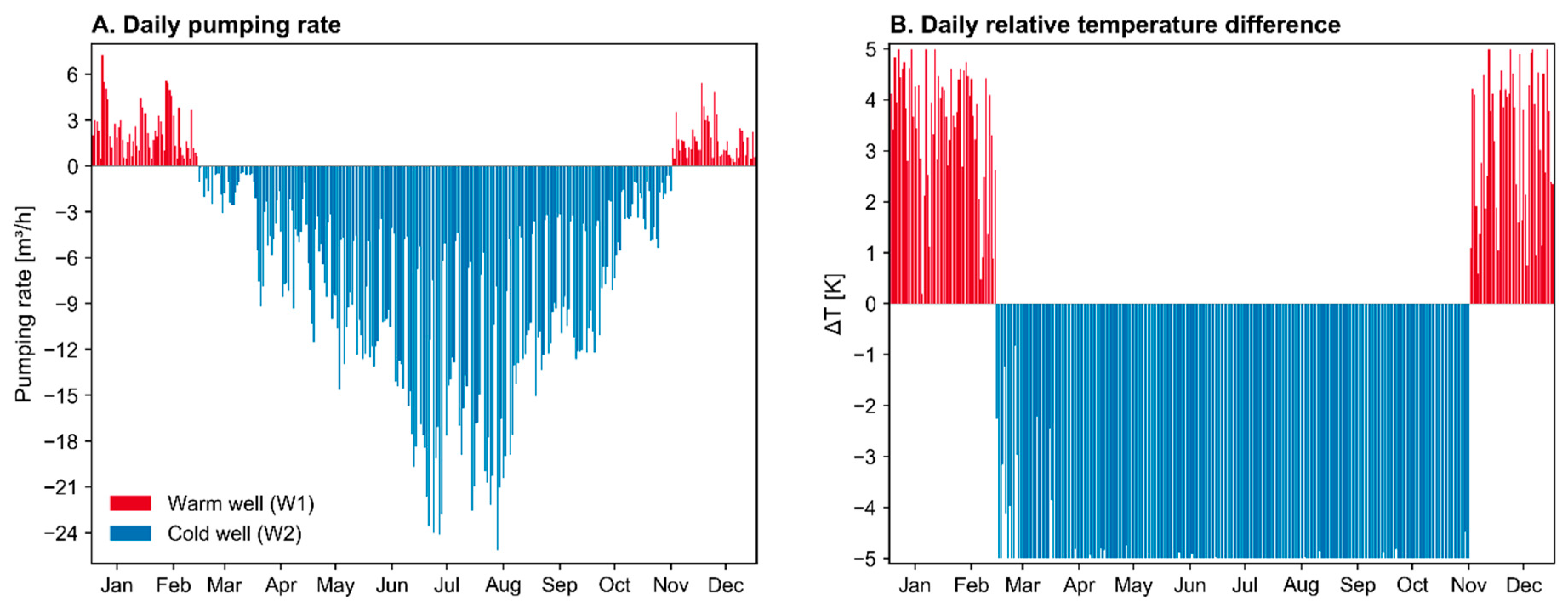
2.6.1. ATES System Operational Characteristics
2.6.2. ATES System Thermal Radii
3. Results
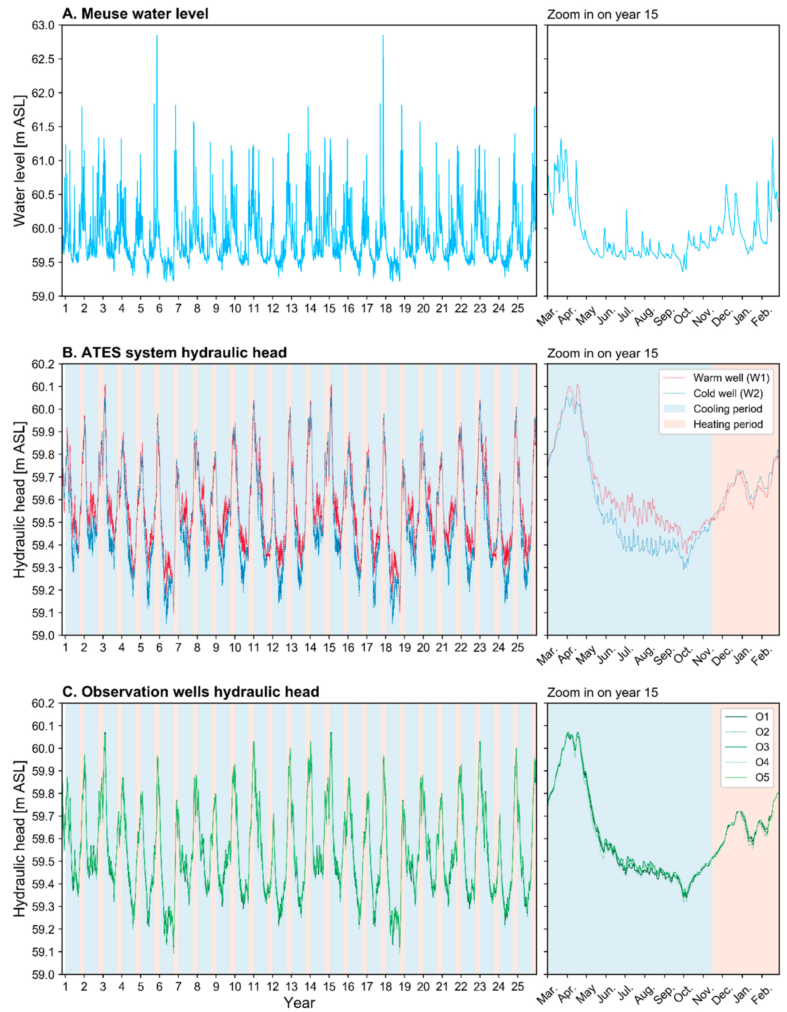
3.1. Groundwater Flow
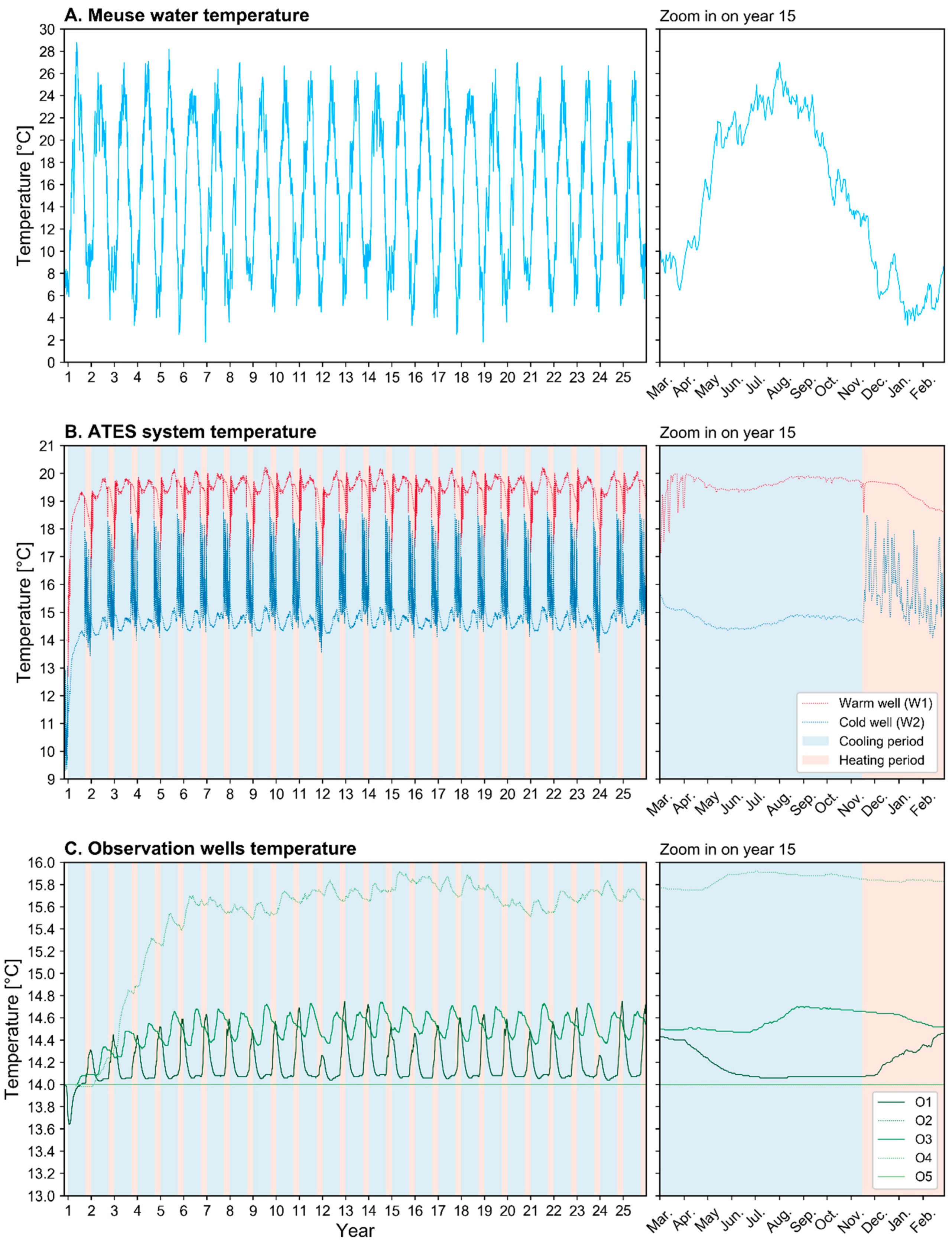
3.2. Groundwater Temperature
4. Discussion
5. Conclusions
Author Contributions
Funding
Acknowledgments
Conflicts of Interest
References
- Dickinson, J.S.; Buik, N.; Matthews, M.C.; Snijders, A. Aquifer thermal energy storage: Theoretical and operational analysis. Géotechnique 2009, 59, 249–260. [Google Scholar] [CrossRef]
- Hesaraki, A.; Holmberg, S.; Haghighat, F. Seasonal thermal energy storage with heat pumps and low temperatures in building projects—A comparative review. Renew. Sustain. Energy Rev. 2015, 43, 1199–1213. [Google Scholar] [CrossRef]
- Fleuchaus, P.; Godschalk, B.; Stober, I.; Blum, P. Worldwide application of aquifer thermal energy storage—A review. Renew. Sustain. Energy Rev. 2018, 94, 861–876. [Google Scholar] [CrossRef]
- Bayer, P.; Saner, D.; Bolay, S.; Rybach, L.; Blum, P. Greenhouse gas emission savings of ground source heat pump systems in Europe: A review. Renew. Sustain. Energy Rev. 2012, 16, 1256–1267. [Google Scholar] [CrossRef]
- Schout, G.; Drijver, B.; Gutierrez-Neri, M.; Schotting, R. Analysis of recovery efficiency in high-temperature aquifer thermal energy storage: A Rayleigh-based method. Hydrogeol. J. 2014, 22, 281–291. [Google Scholar] [CrossRef]
- Andersson, O. Aquifer Thermal Energy Storage (ATES). In Thermal Energy Storage for Sustainable Energy Consumption, 1st ed.; Paksoy, H.Ö., Ed.; Springer: Dordrecht, The Netherlands, 2007; pp. 155–176. ISBN 978-1-4020-5288-0. [Google Scholar]
- Vanhoudt, D.; Desmedt, J.; van Bael, J.; Robeyn, N.; Hoes, H. An aquifer thermal storage system in a Belgian hospital: Long-term experimental evaluation of energy and cost savings. Energy Build. 2011, 43, 3657–3665. [Google Scholar] [CrossRef]
- Hill, M.; DeHouche, Z. A comparative analysis of the effectiveness of aquifer thermal energy storage in expeditionary campaign infrastructure. Appl. Therm. Eng. 2017, 114, 271–278. [Google Scholar] [CrossRef]
- Schüppler, S.; Fleuchaus, P.; Blum, P. Techno-economic and environmental analysis of an Aquifer Thermal Energy Storage (ATES) in Germany. Geotherm. Energy 2019, 7, 11. [Google Scholar] [CrossRef]
- Hartog, N.; Drijver, B.; Dinkla, I.; Bonte, M. Field assessment of the impacts of Aquifer Thermal Energy Storage (ATES) systems on chemical and microbial groundwater composition. In Proceedings of the European Geothermal Conference, Pisa, Italy, 3–7 June 2013. [Google Scholar]
- Bloemendal, M.; Olsthoorn, T.; Boons, F. How to achieve optimal and sustainable use of the subsurface for Aquifer Thermal Energy Storage. Energy Policy 2014, 66, 104–114. [Google Scholar] [CrossRef]
- Andersson, O.; Ekkestubbe, J.; Ekdahl, A. UTES (Underground Thermal Energy Storage)—Applications and market development in Sweden. J. Energy Power Eng. 2013, 7, 669–678. [Google Scholar]
- Wong, B.; Snijders, A. Aquifer Thermal Energy Storage (ATES) applications in Canada. GeoConneXion Mag. 2010, 2010, 30–32. [Google Scholar]
- Sanner, B.; Kabus, F.; Seibt, P.; Bartels, J. Underground thermal energy storage for the German parliament in Berlin, system concept and operational experiences. In Proceedings of the World Geothermal Congress, Antalya, Turkey, 24–29 April 2005. [Google Scholar]
- Chen, H.; Cong, T.N.; Yang, W.; Tan, C.; Li, Y.; Ding, Y. Progress in electrical energy storage system: A critical review. Prog. Nat. Sci. 2009, 19, 291–312. [Google Scholar] [CrossRef]
- Gao, L.; Zhao, J.; Tang, Z. A review on borehole seasonal solar thermal energy storage. Energy Procedia 2015, 70, 209–218. [Google Scholar] [CrossRef]
- Rybach, L.; Kohl, T. Waste heat problems and solutions in geothermal energy. Geol. Soc. Lond. Spec. Publ. 2004, 236, 369–380. [Google Scholar] [CrossRef]
- Lee, K.S. A review on concepts, applications, and models of aquifer thermal energy storage systems. Energies 2010, 3, 1320–1334. [Google Scholar] [CrossRef]
- Xu, J.; Wang, R.Z.; Li, Y. A review of available technologies for seasonal thermal energy storage. Sol. Energy 2014, 103, 610–638. [Google Scholar] [CrossRef]
- Dincer, I. Thermal energy storage systems as a key technology in energy conservation. Int. J. Energy Res. 2002, 26, 567–588. [Google Scholar] [CrossRef]
- Morofsky, E. History of thermal energy storage. In Thermal Energy Storage for Sustainable Energy Consumption, 1st ed.; Paksoy, H.Ö., Ed.; Springer: Dordrecht, The Netherlands, 2007; pp. 3–22. ISBN 978-1-4020-5288-0. [Google Scholar]
- Anibas, C.; Kukral, J.; Possemiers, M.; Huysmans, M. Assessment of seasonal aquifer thermal energy storage as a groundwater ecosystem service for the Brussels-Capital Region: Combining groundwater flow, and heat and reactive transport modeling. Energy Procedia 2016, 97, 179–185. [Google Scholar] [CrossRef]
- Possemiers, M.; Huysmans, M.; Batelaan, O. Influence of aquifer thermal energy storage on groundwater quality: A review illustrated by seven case studies from Belgium. J. Hydrol. Reg. Stud. 2014, 2, 20–34. [Google Scholar] [CrossRef]
- Bolly, P.Y.; Peret, J.; Duren, T.; Wecxsteen, H. Etude hydrogéologique de faisabilité technique d’un projet de chauffage et refroidissement par géothermie du nouveau pôle culturel de Liège—Site Bavière; Technical Report No. R-2017-024; AQUALE: Noville-les-Bois, Belgium, 2017; 137p. (In French) [Google Scholar]
- Pellegrini, M.; Bloemendal, M.; Hoekstra, N.; Spaak, G.; Gallego, A.A.; Comins, J.R.; Grotenhuis, T.; Picone, S.; Murell, A.J.; Steeman, H.J. Low carbon heating and cooling by combining various technologies with Aquifer Thermal Energy Storage. Sci. Total Environ. 2019, 665, 1–10. [Google Scholar] [CrossRef]
- Lund, J.W.; Boyd, T.L. Direct utilization of geothermal energy 2015 worldwide review. Geothermics 2016, 60, 66–93. [Google Scholar] [CrossRef]
- Petitclerc, E.; Laenen, B.; Lagrou, D.; Hoes, H. Geothermal energy use, country update for Belgium. In Proceedings of the European Geothermal Congress 2016, Strasbourg, France, 19–24 September 2016; 7p. [Google Scholar]
- Desmedt, J.; Hoes, H.; van Bael, J. Are underground thermal energy storage projects growing in Belgium? In Proceedings of the 11th International Conference on Thermal Energy Storage for Efficiency and Sustainability (Effstock), Stockholm, Sweden, 14–17 June 2009; 7p. [Google Scholar]
- Loveless, S.; Hoes, H.; Petitclerc, E.; Licour, L.; Laenen, B. Country update for Belgium. In Proceedings of the World Geothermal Congress 2015, Melbourne, Australia, 19–25 April 2015; 6p. [Google Scholar]
- Fossoul, F.; Orban, P.; Dassargues, A. Numerical simulation of heat transfer associated with low enthalpy geothermal pumping in an alluvial aquifer. Geologica Belgica 2011, 14, 45–54. [Google Scholar]
- Wildemeersch, S.; Jamin, P.; Orban, P.; Hermans, T.; Klepikova, M.; Nguyen, F.; Brouyère, S.; Dassargues, A. Coupling heat and chemical tracer experiments for estimating heat transfer parameters in shallow alluvial aquifers. J. Contam. Hydrol. 2014, 169, 90–99. [Google Scholar] [CrossRef]
- Klepikova, M.; Wildemeersch, S.; Hermans, T.; Jamin, P.; Orban, P.; Nguyen, F.; Brouyère, S.; Dassargues, A. Heat tracer test in an alluvial aquifer: Field experiment and inverse modelling. J. Hydrol. 2016, 540, 812–823. [Google Scholar] [CrossRef]
- De Schepper, G.; Paulus, C.; Bolly, P.Y.; Hermans, T.; Lesparre, N.; Robert, T. Short-term aquifer thermal energy storage for demand-side management perspectives: Experimental and numerical developments. Appl. Energy 2019, 242, 534–546. [Google Scholar] [CrossRef]
- Hermans, T.; Lesparre, N.; De Schepper, G.; Robert, T. Bayesian evidential learning: A field validation using push-pull tests. Hydrogeol. J. 2019, 1–12. [Google Scholar] [CrossRef]
- Lesparre, N.; Robert, T.; Nguyen, F.; Boyle, A.; Hermans, T. 4D electrical resistivity tomography (ERT) for aquifer thermal energy storage monitoring. Geothermics 2019, 77, 368–382. [Google Scholar] [CrossRef]
- Robert, T.; Paulus, C.; Bolly, P.Y.; Koo Seen Lin, E.; Hermans, T. Heat as a proxy to image dynamic processes with 4D subsurface thermography. Geosciences 2019, 9, 414. [Google Scholar] [CrossRef]
- Constantz, J. Heat as a tracer to determine streambed water exchanges. Water Resour. Res. 2008, 44, W00D10. [Google Scholar] [CrossRef]
- Trefry, M.G.; Muffels, C. FEFLOW: A finite-element ground water flow and transport modeling tool. Groundwater 2007, 45, 525–528. [Google Scholar] [CrossRef]
- Diersch, H.-J.G. FEFLOW: Finite Element Modeling of Flow, Mass and Heat Transport in Porous and Fractured Media, 1st ed.; Springer: Heidelberg/Berlin, Germany, 2014; 996p. [Google Scholar] [CrossRef]
- Bridger, D.W.; Allen, D.M. Influence of geologic layering on heat transport and storage in an aquifer thermal energy storage system. Hydrogeol. J. 2014, 22, 233–250. [Google Scholar] [CrossRef]
- Stefansson, V. Geothermal reinjection experience. Geothermics 1997, 26, 99–139. [Google Scholar] [CrossRef]
- Ferguson, G.; Woodbury, A.D. Thermal sustainability of groundwater-source cooling in Winnipeg, Manitoba. Can. Geotech. J. 2005, 42, 1290–1301. [Google Scholar] [CrossRef]
- Milnes, E.; Perrochet, P. Assessing the impact of thermal feedback and recycling in open-loop groundwater heat pump (GWHP) systems: A complementary design tool. Hydrogeol. J. 2013, 21, 505–514. [Google Scholar] [CrossRef]
- Sheldon, H.A.; Schaubs, P.M.; Rachakonda, P.K.; Trefry, M.G.; Reid, L.B.; Lester, D.R.; Metcalfe, G.; Poulet, T.; Regenauer-Lieb, K. Groundwater cooling of a supercomputer in Perth, Western Australia: Hydrogeological simulations and thermal sustainability. Hydrogeol. J. 2015, 23, 1831–1849. [Google Scholar] [CrossRef]
- Ganguly, S.; Kumar, M.M.; Date, A.; Akbarzadeh, A. Numerical investigation of temperature distribution and thermal performance while charging-discharging thermal energy in aquifer. Appl. Therm. Eng. 2017, 115, 756–773. [Google Scholar] [CrossRef]
- Vandenbohede, A.; Hermans, T.; Nguyen, F.; Lebbe, L. Shallow heat injection and storage experiment: Heat transport simulation and sensitivity analysis. J. Hydrol. 2011, 69, 262–272. [Google Scholar] [CrossRef]
- Arola, T.; Okkonen, J.; Jokisalo, J. Groundwater utilisation for energy production in the Nordic environment: An energy simulation and hydrogeological modelling approach. J. Water Resour. Prot. 2016, 8, 642–656. [Google Scholar] [CrossRef][Green Version]
- Sommer, W.T.; Doornenbal, P.J.; Drijver, B.C.; van Gaans, P.F.M.; Leusbrock, I.; Grotenhuis, J.T.C.; Rijnaarts, H.H.M. Thermal performance and heat transport in aquifer thermal energy storage. Hydrogeol. J. 2014, 22, 263–279. [Google Scholar] [CrossRef]
- Ferguson, G. Heterogeneity and thermal modeling of ground water. Groundwater 2007, 45, 485–490. [Google Scholar] [CrossRef]
- Ruthy, I.; Dassargues, A. Carte Hydrogéologique de Wallonie, Alleur-Liège (42/1-2); Service Public de Wallonie: Jambes, Belgium, 2009; ISBN 978-2-8056005-3-1. (In French) [Google Scholar]
- Theis, C.V. The relation between the lowering of the piezometric surface and the rate and duration of discharge of a well using groundwater storage. Trans. Am. Geophys. Union 1935, 2, 519–524. [Google Scholar] [CrossRef]
- Renard, P. Hydraulics of well and well testing. In Encyclopedia of Hydrological Sciences, 1st ed.; Anderson, M.G., Ed.; Wiley: New York, NY, USA, 2005; pp. 2323–2340. [Google Scholar]
- Dassargues, A. Modeling baseflow from an alluvial aquifer using hydraulic-conductivity data obtained from a derived relation with apparent electrical resistivity. Hydrogeol. J. 1997, 5, 97–108. [Google Scholar] [CrossRef]
- Bloemendal, M.; Hartog, N. Analysis of the impact of storage conditions on the thermal recovery efficiency of low-temperature ATES systems. Geothermics 2018, 71, 306–319. [Google Scholar] [CrossRef]
- Bloemendal, M.; Jaxa-Rozen, M.; Olsthoorn, T. Methods for planning of ATES systems. Appl. Energy 2018, 216, 534–557. [Google Scholar] [CrossRef]
- Robert, T.; Hermans, T.; Lesparre, N.; De Schepper, G.; Nguyen, F.; Defourny, A.; Orban, P.; Brouyère, S.; Dassargues, A. Towards a subsurface predictive-model environment to simulate aquifer thermal energy storage for demand-side management applications. In Proceedings of the 10th International Conference on System Simulation in Buildings (SSB2018), Liège, Belgium, 10–12 December 2018; p. 18. [Google Scholar]
- Schnegg, P.A. An inexpensive field fluorometer for hydrogeological tracer tests with three tracers and turbidity measurement. Articles of the Geomagnetism Group at the University of Neuchâtel, Groundwater and Human Development. 2002, pp. 1484–1488. Available online: http://doc.rero.ch/record/5068 (accessed on 19 January 2020).
- Becker, M.W.; Shapiro, A.M. Interpreting tracer breakthrough tailing from different forced-gradient tracer experiment configurations in fractured bedrock. Water Resour. Res. 2003, 39, 1014. [Google Scholar] [CrossRef]
- Dassargues, A.; Wildemeersch, S.; Rentier, C. Graviers de la Meuse (alluvions modernes et anciennes) en Wallonie. In Watervoerende lagen & grondwater in België—Aquifères & eaux souterraines en Belgique; Dassargues, A., Walraevens, K., Eds.; Academia Press: Ghent, Belgium, 2014; pp. 37–46. ISBN 978-9-0382236-4-3. (In French) [Google Scholar]
- Epting, J.; Händel, F.; Huggenberger, P. Thermal management of an unconsolidated shallow urban groundwater body. Hydrol. Earth. Syst. Sc. 2013, 17, 1851–1869. [Google Scholar] [CrossRef]
- Somogyvári, M.; Bayer, P.; Brauchler, R. Travel-time-based thermal tracer tomography. Hydrol. Earth. Syst. Sc. 2016, 20, 1885–1901. [Google Scholar] [CrossRef]
- Molson, J.W.; Frind, E.O.; Palmer, C.D. Thermal energy storage in an unconfined aquifer: 2. Model development, validation, and application. Water Resour. Res. 1992, 28, 2857–2867. [Google Scholar] [CrossRef]
- Engie Electrabel. Centrale Nucléaire de Thiange: Déclaration Environnementale 2018; Engie Electrabel Public Report; Electrabel SA: Brussels, Belgium, 2018; 69p, (In French). Available online: http://corporate.engie-electrabel.be/wp-content/uploads/2018/08/cnt-declaration-environnementale-2018.pdf (accessed on 16 February 2019).
- Doherty, J. Calibration and Uncertainty Analysis for Complex Environmental Models; Watermark Numerical Computing: Brisbane, Australia, 2015; 227p, ISBN 978-0-9943786-0-6. [Google Scholar]
- Doherty, J. PEST: Model-Independent Parameter Estimation, User Manual, 6th ed.; Watermark Numerical Computing: Brisbane, Australia, 2016. [Google Scholar]
- De Marsily, G. De L’identification des Systèmes Hydrogéologiques. Ph.D. Thesis, Ecole des Mines de Paris, Centre d’Informatique Géologique, Paris, France, December 1978. (In French). [Google Scholar]
- Renard, P. Stochastic hydrogeology: What professionals really need? Groundwater 2007, 45, 531–541. [Google Scholar] [CrossRef]
- Irvine, D.J.; Simmons, C.T.; Werner, A.D.; Graf, T. Heat and solute tracers: How do they compare in heterogeneous aquifers? Groundwater 2015, 53, 10–20. [Google Scholar] [CrossRef]
- Doughty, C.; Hellström, G.; Tsang, C.F.; Claesson, J. A dimensionless parameter approach to the thermal behavior of an aquifer thermal energy storage system. Water Resour. Res. 1982, 18, 571–587. [Google Scholar] [CrossRef]
- Attard, G.; Rossier, Y.; Winiarski, T.; Eisenlohr, L. Deterministic modeling of the impact of underground structures on urban groundwater temperature. Sci. Total Environ. 2016, 572, 986–994. [Google Scholar] [CrossRef] [PubMed]
- Moore, C.; Doherty, J. The cost of uniqueness in groundwater model calibration. Adv. Water Resour. 2006, 29, 605–623. [Google Scholar] [CrossRef]
- Maneta, M.P.; Wallender, W.W. Pilot-point based multi-objective calibration in a surface–subsurface distributed hydrological model. Hydrol. Sci. J. 2013, 58, 390–407. [Google Scholar] [CrossRef]
- Tordrup, K.W.; Poulsen, S.E.; Bjørn, H. An improved method for upscaling borehole thermal energy storage using inverse finite element modelling. Renew. Energy 2017, 105, 13–21. [Google Scholar] [CrossRef]
- Moeck, C.; Molson, J.; Schirmer, M. Pathline density distributions in a Null-Space Monte Carlo approach to assess groundwater pathways. Groundwater 2019. [Google Scholar] [CrossRef]
- Anderson, M.P. Heat as a ground water tracer. Groundwater 2005, 43, 951–968. [Google Scholar] [CrossRef]
- Schilling, O.S.; Cook, P.G.; Brunner, P. Beyond classical observations in hydrogeology: The advantages of including exchange flux, temperature, tracer concentration, residence time, and soil moisture observations in groundwater model calibration. Rev. Geophys. 2019, 57, 146–182. [Google Scholar] [CrossRef]
- Gianni, G.; Doherty, J.; Brunner, P. Conceptualization and calibration of anisotropic alluvial systems: Pitfalls and biases. Groundwater 2019, 57, 409–419. [Google Scholar] [CrossRef]
- Bloemendal, M.; Olsthoorn, T. ATES systems in aquifers with high ambient groundwater flow velocity. Geothermics 2019, 75, 81–92. [Google Scholar] [CrossRef]
- Rentier, C.; Brouyère, S.; Dassargues, A. Calibration and reliability of an alluvial aquifer model using inverse modelling and sensitivity analysis. In Proceedings of the ModelCARE’99, Zurich, Switzerland, 20–23 September 1999; pp. 343–348. [Google Scholar]
- Epting, J.; Huggenberger, P.; Rauber, M. Integrated methods and scenario development for urban groundwater management and protection during tunnel road construction: A case study of urban hydrogeology in the city of Basel, Switzerland. Hydrogeol. J. 2008, 16, 575–591. [Google Scholar] [CrossRef]
- Schirmer, M.; Leschik, S.; Musolff, A. Current research in urban hydrogeology—A review. Adv. Water Resour. 2013, 51, 280–291. [Google Scholar] [CrossRef]
- Attard, G.; Winiarski, T.; Rossier, Y.; Eisenlohr, L. Review: Impact of underground structures on the flow of urban groundwater. Hydrogeol. J. 2015, 24, 5–19. [Google Scholar] [CrossRef]
- García-Gil, A.; Vázquez-Suñe, E.; Schneider, E.G.; Sánchez-Navarro, J.Á.; Mateo-Lázaro, J. The thermal consequences of river-level variations in an urban groundwater body highly affected by groundwater heat pumps. Sci. Total Environ. 2014, 485, 575–587. [Google Scholar] [CrossRef] [PubMed]
- Hermans, T.; Wildemeersch, S.; Jamin, P.; Orban, P.; Brouyère, S.; Dassargues, A.; Nguyen, F. Quantitative temperature monitoring of a heat tracing experiment using cross-borehole ERT. Geothermics 2015, 53, 14–26. [Google Scholar] [CrossRef]
- Benz, S.A.; Bayer, P.; Blum, P. Identifying anthropogenic anomalies in air, surface and groundwater temperatures in Germany. Sci. Total Environ. 2017, 584, 145–153. [Google Scholar] [CrossRef]
- Allen, A.; Milenić, D.; Sikora, P. Shallow gravel aquifers and the urban heat island effect: A source of low enthalpy geothermal energy. Geothermics 2003, 32, 569–578. [Google Scholar] [CrossRef]
- Ferguson, G.; Woodbury, A.D. Urban heat island in the subsurface. Geophys. Res. Lett. 2007, 34, L23713. [Google Scholar] [CrossRef]
- Epting, J.; Huggenberger, P. Unraveling the heat island effect observed in urban groundwater bodies—Definition of a potential natural state. J. Hydrol. 2013, 501, 193–204. [Google Scholar] [CrossRef]
- Menberg, K.; Bayer, P.; Zosseder, K.; Rumohr, S.; Blum, P. Subsurface urban heat islands in German cities. Sci. Total Environ. 2013, 442, 123–133. [Google Scholar] [CrossRef]
- Bayer, P.; Attard, G.; Blum, P.; Menberg, K. The geothermal potential of cities. Renew. Sustain. Energy Rev. 2019, 106, 17–30. [Google Scholar] [CrossRef]
- Arola, T.; Korkka-Niemi, K. The effect of urban heat islands on geothermal potential: Examples from Quaternary aquifers in Finland. Hydrogeol. J. 2014, 22, 1953–1967. [Google Scholar] [CrossRef]
- Benz, S.A.; Bayer, P.; Menberg, K.; Jung, S.; Blum, P. Spatial resolution of anthropogenic heat fluxes into urban aquifers. Sci. Total Environ. 2015, 524, 427–439. [Google Scholar] [CrossRef] [PubMed]
- Menberg, K.; Blum, P.; Schaffitel, A.; Bayer, P. Long-term evolution of anthropogenic heat fluxes into a subsurface urban heat island. Environ. Sci. Technol. 2013, 47, 9747–9755. [Google Scholar] [CrossRef]
- Mueller, M.H.; Huggenberger, P.; Epting, J. Combining monitoring and modelling tools as a basis for city-scale concepts for a sustainable thermal management of urban groundwater resources. Sci. Total Environ. 2018, 627, 1121–1136. [Google Scholar] [CrossRef]
- Anibas, C.; Fleckenstein, J.H.; Volze, N.; Buis, K.; Verhoeven, R.; Meire, P.; Batelaan, O. Transient or steady-state? Using vertical temperature profiles to quantify groundwater–surface water exchange. Hydrol. Process. 2009, 23, 2165–2177. [Google Scholar] [CrossRef]


| Heat Tracer | Dye Tracer | |
|---|---|---|
| Volume/Concentration | 28 m3 (+34 K) | 50 L (20 g/L) |
| First arrival | 9.2 h | 1.7 h |
| Peak time | 31.2 h | 3.0 h |
| Maximum flow velocity | 1.8 m/h | 9.4 m/h |
| Peak flow velocity | 0.5 m/h | 5.3 m/h |
| Parameter | Initial | Calibrated | Reference |
|---|---|---|---|
| Horizontal hydraulic conductivity [m·s−1] | 5.3 × 10⁻³ | 2.1 × 10⁻² to 3.0 × 10⁻⁴ | Pumping tests |
| Vertical hydraulic conductivity [m·s−1] | 5.3 × 10⁻⁴ | 2.1 × 10⁻³ to 3.0 × 10⁻⁵ | Pumping tests |
| Specific storage [m−1] | 1.2 × 10⁻³ | - | Pumping tests |
| Effective porosity [-] | 0.12 | 0.16 a | [60] |
| Matrix heat capacity [MJ·m−3 K−1] | 2.87 | 2.27 b | [61] |
| Matrix thermal conductivity [J·m−1·s−1·K−1] | 2.7 | 2.7 b | [61] |
| Longitudinal dispersivity [m] | 20 | 10 | [60] |
| Transverse dispersivity [m] | 2 | 1 | [60] |
| Parameter | Loamy Backfill Soil | Reference | Silty Aquitard | Reference |
|---|---|---|---|---|
| Horizontal hydraulic conductivity [m·s−1] | 1.0 × 10⁻⁴ | [32] | 2.0 × 10⁻⁶ | [32] |
| Vertical hydraulic conductivity [m·s−1] | 1.0 × 10⁻⁵ | [32] | 2.0 × 10⁻⁷ | [32] |
| Specific storage [m−1] | 1.0 × 10⁻⁴ | [32] | 1.0 × 10⁻⁴ | [32] |
| Effective porosity [-] | 0.05 | [32] | 0.02 | [32] |
| Matrix heat capacity [MJ·m−3 K−1] | 3.0 | [57] | 2.22 | [31] |
| Matrix thermal conductivity [J·m−1·s−1·K−1] | 1.9 | [57] | 1.37 | [31] |
| Longitudinal dispersivity [m] | 5 | [32] | 5 | [32] |
| Transverse dispersivity [m] | 0.5 | [32] | 0.5 | [32] |
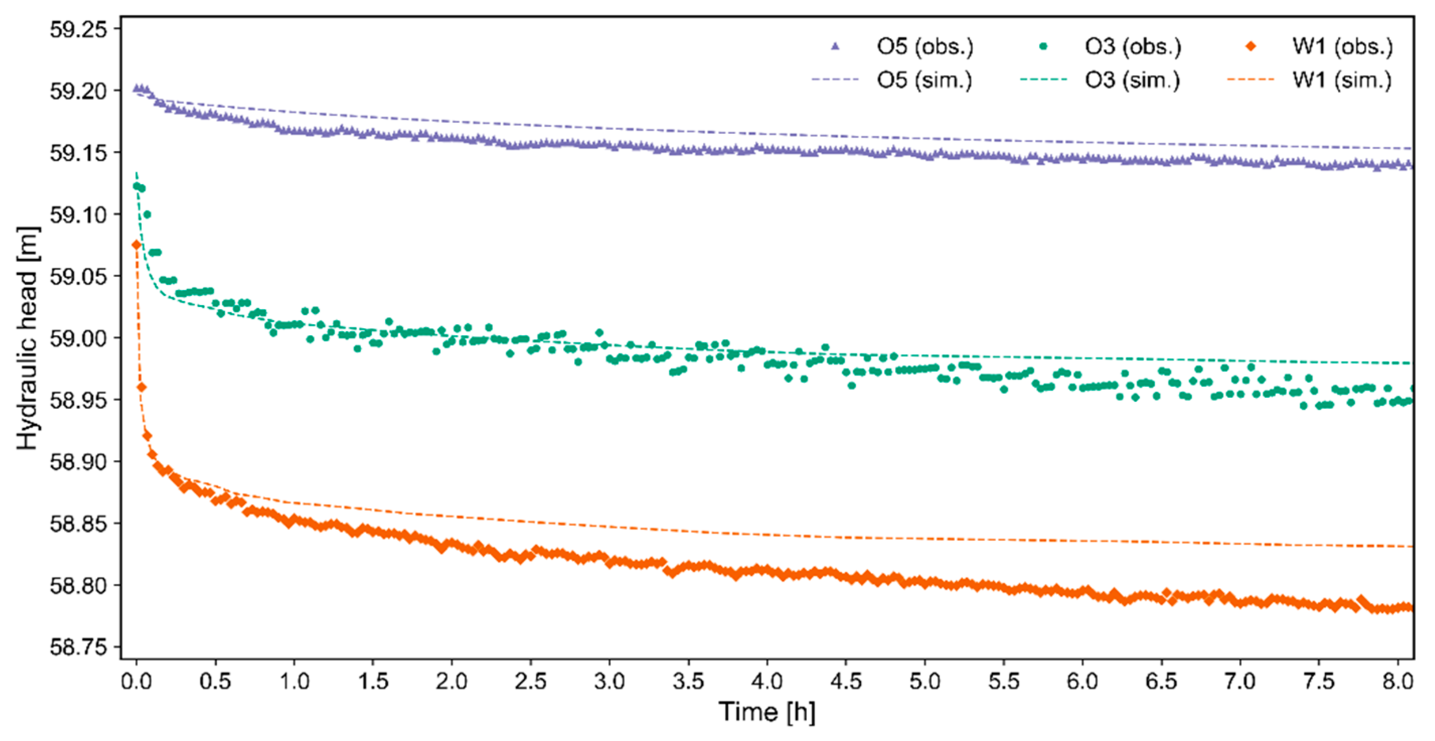
| Observed (m) | Simulated (m) | Residual (m) | |
|---|---|---|---|
| O1 | 59.21 | 59.21 | 0.00 |
| O2 | 59.21 | 59.22 | 0.01 |
| O3 | 59.19 | 59.18 | -0.01 |
| O4 | 59.18 | 59.16 | -0.02 |
| O5 | 59.23 | 59.23 | -0.01 |
| Warm Well (W1) | Cold Well (W2) | |||||
|---|---|---|---|---|---|---|
| Vin [m3] | Rth [m] | L/Rth [-] | Vin [m3] | Rth [m] | L/Rth [-] | |
| January | - | - | - | 1890 | 14.5 | 0.24 |
| February | - | - | - | 1430 | 12.6 | 0.28 |
| March | 585 | 5.9 | 1.10 | - | - | - |
| April | 3552 | 14.6 | 0.44 | - | - | - |
| May | 6170 | 19.3 | 0.34 | - | - | - |
| June | 7588 | 21.4 | 0.30 | - | - | - |
| July | 11,261 | 26.0 | 0.25 | - | - | - |
| August | 10,213 | 24.8 | 0.26 | - | - | - |
| September | 6411 | 19.6 | 0.33 | - | - | - |
| October | 3819 | 15.2 | 0.43 | - | - | - |
| November | 1315 | 8.9 | 0.73 | - | - | - |
| December | - | - | - | 59.23 | 14.5 | 0.24 |
© 2020 by the authors. Licensee MDPI, Basel, Switzerland. This article is an open access article distributed under the terms and conditions of the Creative Commons Attribution (CC BY) license (http://creativecommons.org/licenses/by/4.0/).
Share and Cite
De Schepper, G.; Bolly, P.-Y.; Vizzotto, P.; Wecxsteen, H.; Robert, T. Investigations into the First Operational Aquifer Thermal Energy Storage System in Wallonia (Belgium): What Can Potentially Be Expected? Geosciences 2020, 10, 33. https://doi.org/10.3390/geosciences10010033
De Schepper G, Bolly P-Y, Vizzotto P, Wecxsteen H, Robert T. Investigations into the First Operational Aquifer Thermal Energy Storage System in Wallonia (Belgium): What Can Potentially Be Expected? Geosciences. 2020; 10(1):33. https://doi.org/10.3390/geosciences10010033
Chicago/Turabian StyleDe Schepper, Guillaume, Pierre-Yves Bolly, Pietro Vizzotto, Hugo Wecxsteen, and Tanguy Robert. 2020. "Investigations into the First Operational Aquifer Thermal Energy Storage System in Wallonia (Belgium): What Can Potentially Be Expected?" Geosciences 10, no. 1: 33. https://doi.org/10.3390/geosciences10010033
APA StyleDe Schepper, G., Bolly, P.-Y., Vizzotto, P., Wecxsteen, H., & Robert, T. (2020). Investigations into the First Operational Aquifer Thermal Energy Storage System in Wallonia (Belgium): What Can Potentially Be Expected? Geosciences, 10(1), 33. https://doi.org/10.3390/geosciences10010033