Article

Uncertainty Assessment of Ice Discharge Using GPR-Derived Ice Thickness from Gourdon Glacier, Antarctic Peninsula

by
Stefan Lippl
1,*,
Norbert Blindow
1,
Johannes J. Fürst
1,
Sebastián Marinsek
2,
Thorsten C. Seehaus
1 and
Matthias H. Braun
1
1
Institut für Geographie, Friedrich-Alexander-Universität Erlangen-Nürnberg, Wetterkreuz 15, 91052 Erlangen, Germany
2
Instituto Antártico Argentino, 25 de Mayo 1143, San Martín 1650, Argentina
*
Author to whom correspondence should be addressed.
Geosciences 2020, 10(1), 12; https://doi.org/10.3390/geosciences10010012
Submission received: 11 November 2019 / Revised: 16 December 2019 / Accepted: 23 December 2019 / Published: 27 December 2019
(This article belongs to the Section Hydrogeology)

Abstract

:
Ice cliffs within a glacier represent a challenge for the continuity equations used in many glacier models by interrupting the validity of input parameters. In the case of Gourdon Glacier on James Ross Island, Antarctica, a ∼300–500 m high, almost vertical cliff, separates the outlet glacier from its main accumulation area on the plateau of the island. In 2017 and 2018 we conducted ice thickness measurements during two airborne ground penetrating radar campaigns in order to evaluate differences to older measurements from the 1990s. The observed differences are mostly smaller than the estimated error bars. In comparison to the in situ data, the published “consensus ice thickness estimate” strongly overestimates the ice thickness at the outlet. We analyse three different interpolation and ice thickness reconstruction methods. One approach additionally includes the mass input from the plateau. Differences between the interpolation methods have a minor impact on the ice discharge estimation if the used flux gates are in areas with a good coverage of in situ measurements. A much stronger influence was observed by uncertainties in the glacier velocities derived from remote sensing, especially in the direction of the velocity vector in proximity to the ice cliff. We conclude that the amount of in situ measurements should be increased for specific glacier types in order to detect biases in modeled ice thickness and ice discharge estimations.

Graphical Abstract

1. Introduction

In order to forecast glacier run-off and the potential contribution to sea-level rise, an accurate estimation of the overall ice volume, but also the ice thickness distribution, is essential [1,2]. However, there still exists a large lack in data availability. The Glacier Thickness Database [3] published by the World Glacier Monitoring Service contains information for only ∼1000 out of the overall ∼215,000 glaciers outside of the Greenland and Antarctic ice sheets [4], with data for only seven glaciers in the Antarctica [3]. Therefore, a wide spectrum of techniques has been developed do infer glacier volume from surface characteristics. Beside volume–area scaling (e.g., [5,6]), techniques have been developed that make use of surface velocity information (e.g., [7]), parameterisations of the basal shear stress (e.g., [8,9,10,11]) or mass conservation (e.g., [12,13,14]). Other approaches cast the thickness reconstruction as a minimisation problem (e.g., [15,16,17]). Results from the Ice Thickness Models Intercomparison eXperiment (ITMIX, [18]) revealed that pooling the results from several models can significantly reduce the associated uncertainty as compared to individual results. They combined outcomes of five ice thickness estimation models (for the Randolph Glacier Inventory (RGI) region 19/Antarctic and subantarctic only 1–2) to one ensemble-based “consensus ice thickness estimate” (CIE) [4,19] for each of the glaciers included in the RGI [20]. Nevertheless, peculiarities in the glacier geometry, but also local variations in the morphology of the bedrock, are still difficult to treat due to the lower resolution of input data (e.g., 7 . 5 km in the Modèle Atmosphérique Régional (MAR) applied in this study for the simulation of the surface mass balance (SMB) [21,22,23]). Moreover, ice cliffs exceeding several meters interrupt the continuity equations along flow lines and impose a boundary condition on the ice flux and ice thickness. Yet, along the ice cliff both values are non-zero. In case of marine-terminating Gourdon Glacier (James Ross Island (JRI), Antarctic Peninsula, Figure 1a,b), large parts of the accumulation area are separated from the outlet glacier by a ∼300–500 m high, almost vertical cliff. The transfer of mass from the upper plateau to the lower glacier trunk by ice avalanches is sporadic and not predictable by us in time.
Many approaches participating in ITMIX use the difference between their simulated SMB and the contemporaneous surface elevation changes, also referred as the apparent mass balance [12,17]. However, climate parameters like the SMB abruptly change at the cliff by the large height difference. In situ measurements for Gourdon Glacier reveal that these values can differ between approximately + 0 . 5 m w . e . a 1 on the plateau and negative rates up to 3 m w . e . a 1 on the outlet part. Sensitivity tests for different SMB input data revealed a strong influence on the ice thickness reconstruction [17]. Even if the averaged values of current models reflect the real ice volumes correctly over larger areas, the application of the results for smaller areas such as Gourdon Glacier (∼10 km length and 2 km width) is limited [4]. Thus, validation with in situ data remains an indispensable requisite to evaluate any biases for specific glacier types.
The scope of this study is an evaluation of differences in ice thickness and their influence on ice discharge between the CIE data and in situ measurements derived from ground penetrating radar (GPR) for the cliff-separated glacier type of Gourdon Glacier. For the estimation of ice discharge, we use velocity estimates calculated with radar images from TerraSAR-X and TanDEM-X satellite missions. To answer the question, this study aims at
(1)
describing new ice thickness measurements on JRI;
(2)
assessing the influence of different ice thickness interpolation and reconstruction methods;
(3)
evaluating uncertainties in ice discharge of Gourdon Glacier in dependence on the location of the flux gate;
(4)
integrating the mass input by ice avalanches from the plateau into one ice thickness reconstruction method.
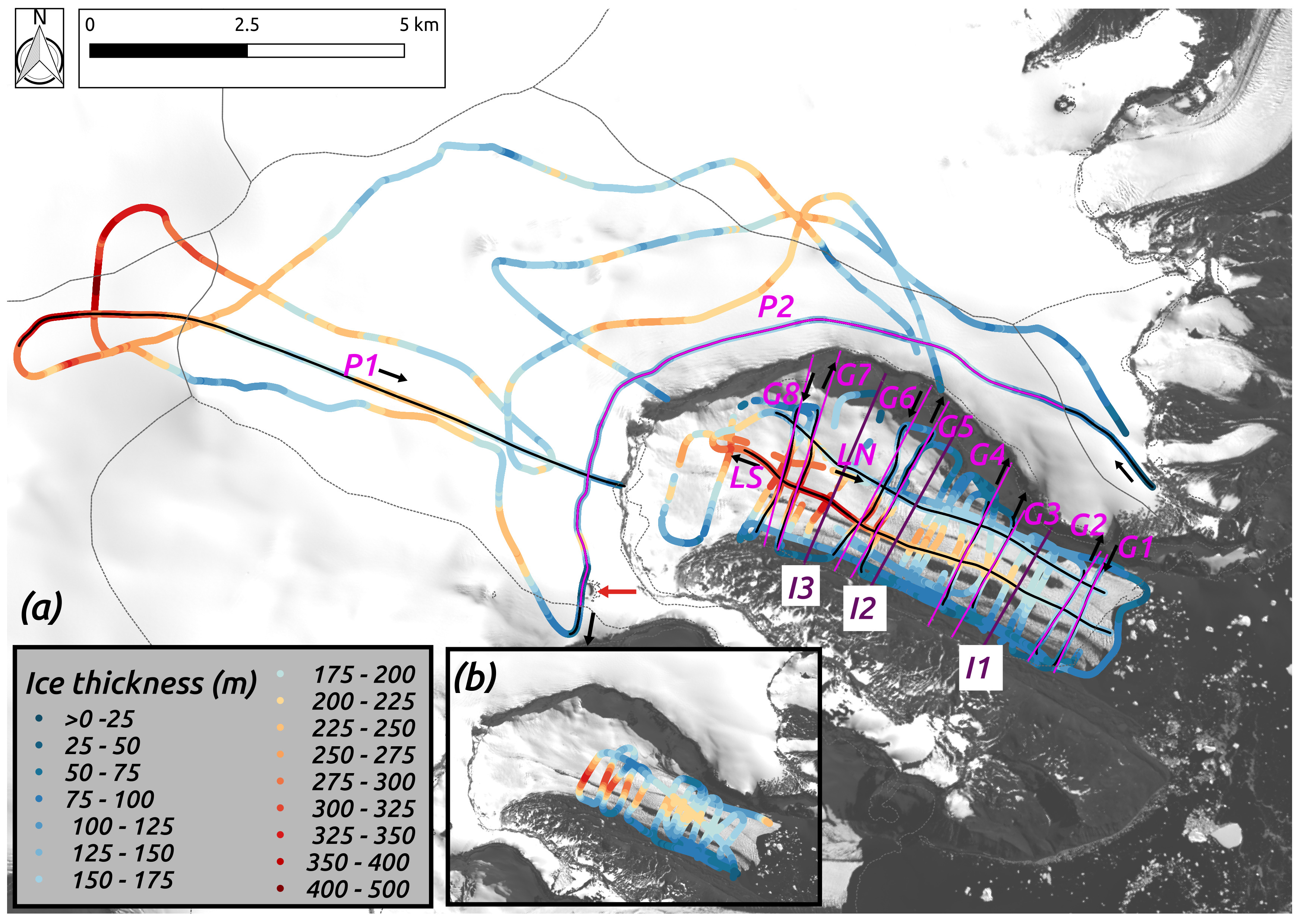
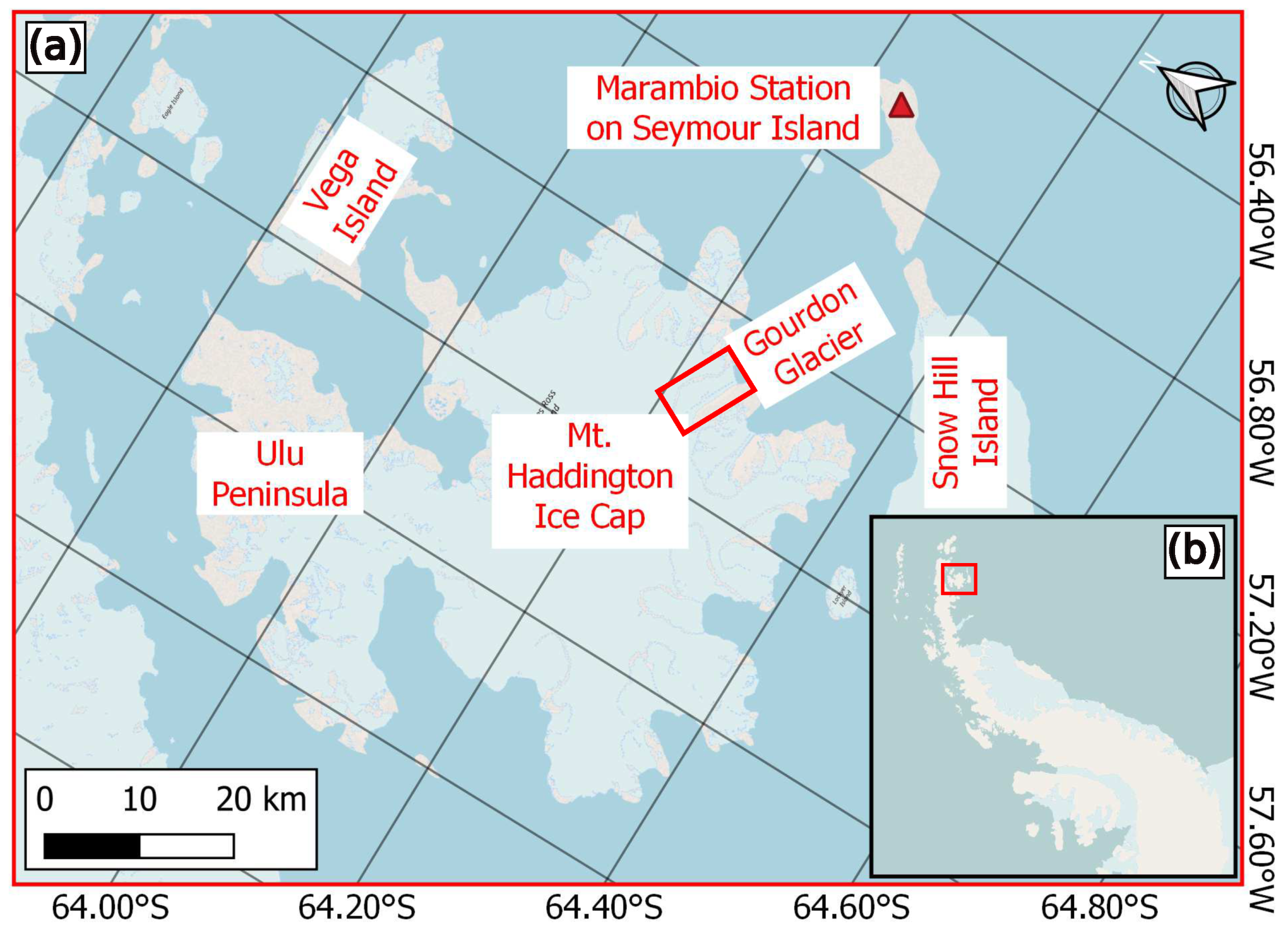
2. Study Site

JRI is located on the eastern side of the northern Antarctic Peninsula (Figure 1a,b). The island is ∼2500 km 2 large of which three quarters are covered by ice [24]. The main part of the island and the main outlet glaciers are dominated by the Mount Haddington Ice Cap, whereas the Ulu Peninsula at the northern part of JRI has considerable ice free areas (Figure 1a). JRI consists of resistant volcanic rock overlying soft Cretaceous sediments [25]. Therefore, most of the marine-terminating outlet glaciers draining the Mount Haddington Ice Cap are separated from the accumulation areas on the plateau by a sharp change in slope at cirque headwalls or cliffs [24]. The glacier trunks at lower elevation typically show gentle slopes and are recognized to be vulnerable to changes in the equilibrium line altitude.

3. Materials and Methods

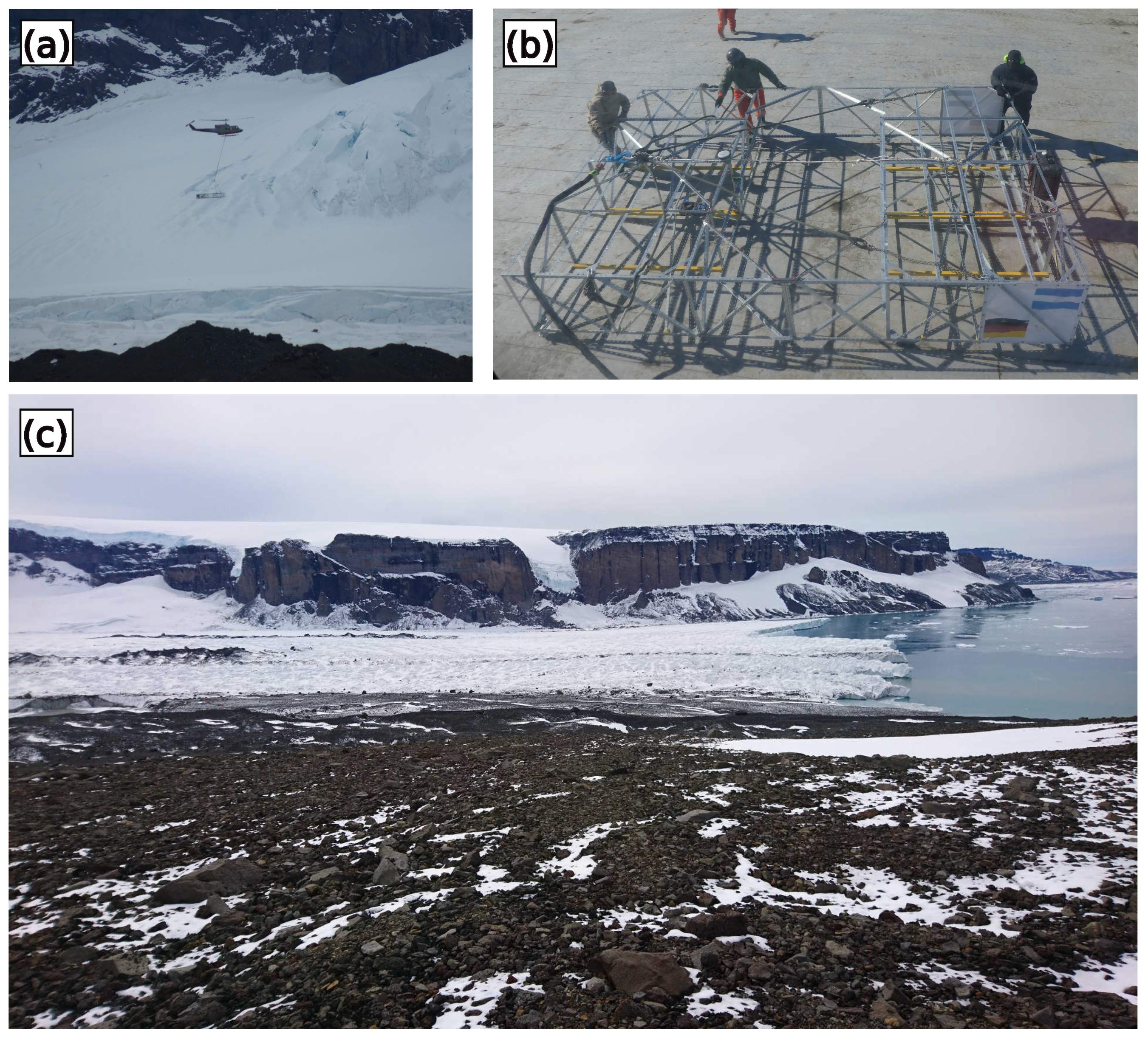
3.1. In Situ Ice Thickness Measurements

In order to improve ice discharge estimates, airborne GPR campaigns were conducted on Gourdon Glacier in February 2017 and February 2018. A 25 MHz GPR system with a L1/L2 differential Global Navigation Satellite System (GNSS), a laser altimeter (Universal Laser Sensor from Laser Technology Inc., Centennial, Colorado, CO 80112, USA), and an Inertial Measurement Unit (Xsens MTi) for a precise geolocation were flown as a sling load by a Bell 212 helicopter (Figure A1). The basic system design was oriented on the BGR-P30 (formerly UMAIR, [26]) and its performance was tested in Blindow et al. [27] at Nef and Colonia Glaciers in Patagonia. The GPR uses a pair of shielded broadband antennas for transmitting and receiving hanging ∼20 m below the helicopter. Their self-contained mechanical structure is carrying battery powered GPR electronics (Unmanned Inc., 5090000 Valdivia, Chile) and the additional sensors mentioned above. A fiberoptic link connects to the control unit inside the helicopter. GPR measurements of the surface and bedrock reflections were collected with a ∼2 m sampling interval at the outlet and catchment area of Gourdon Glacier. At the outlet, profiles were flown mostly transverse to the main glacier flow direction. Due to the ambiguity of possible reflector locations for profiles along glacier flow, longitudinal measurements were done only in the middle of the glacier where no backscatter from the side walls arrived previous to the bedrock reflection [28]. At the catchment area on the plateau of the island we conducted measurements with the aim to include repetitions of profiles flown by previous ice thickness surveys in the years 1995/96 and 1997/98. These earlier datasets were obtained by radio echo sounding using a linear frequency modulation (chirp) waveform with 10 MHz bandwidth and a position accuracy of 0.2–0.5 m (UK-ARG 9596 and UK-ARG 9798, data from AWI/BAS Bedmap 1 mission summary). However, higher elevations (∼1500 m a . s . l . ) and difficult wind conditions on the plateau limited the measurements, resulting in a sparse profile pattern. The lower density of measurements does not allows an interpolation over the whole catchment area with sufficient accuracy. Thus, the estimation of ice discharge was done only directly along in situ measurements.

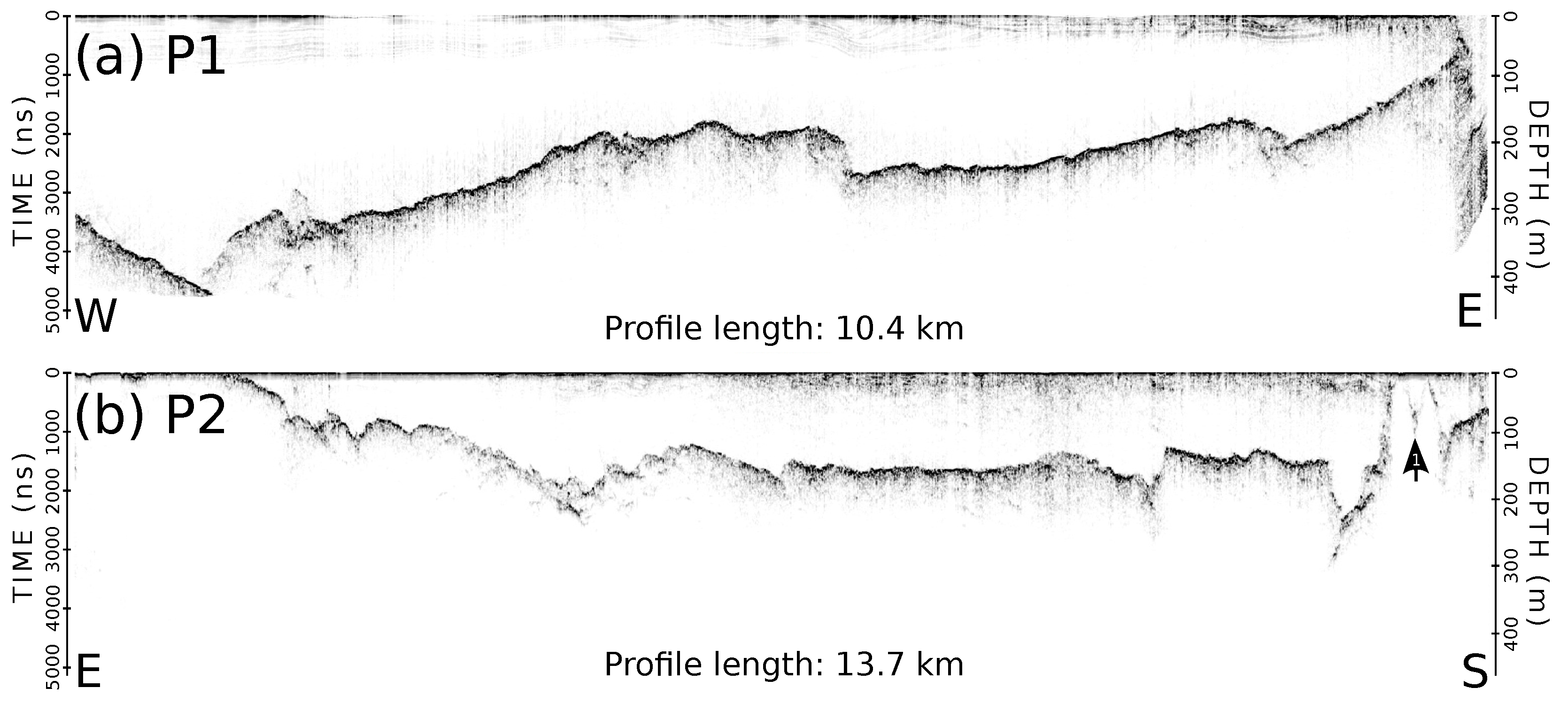
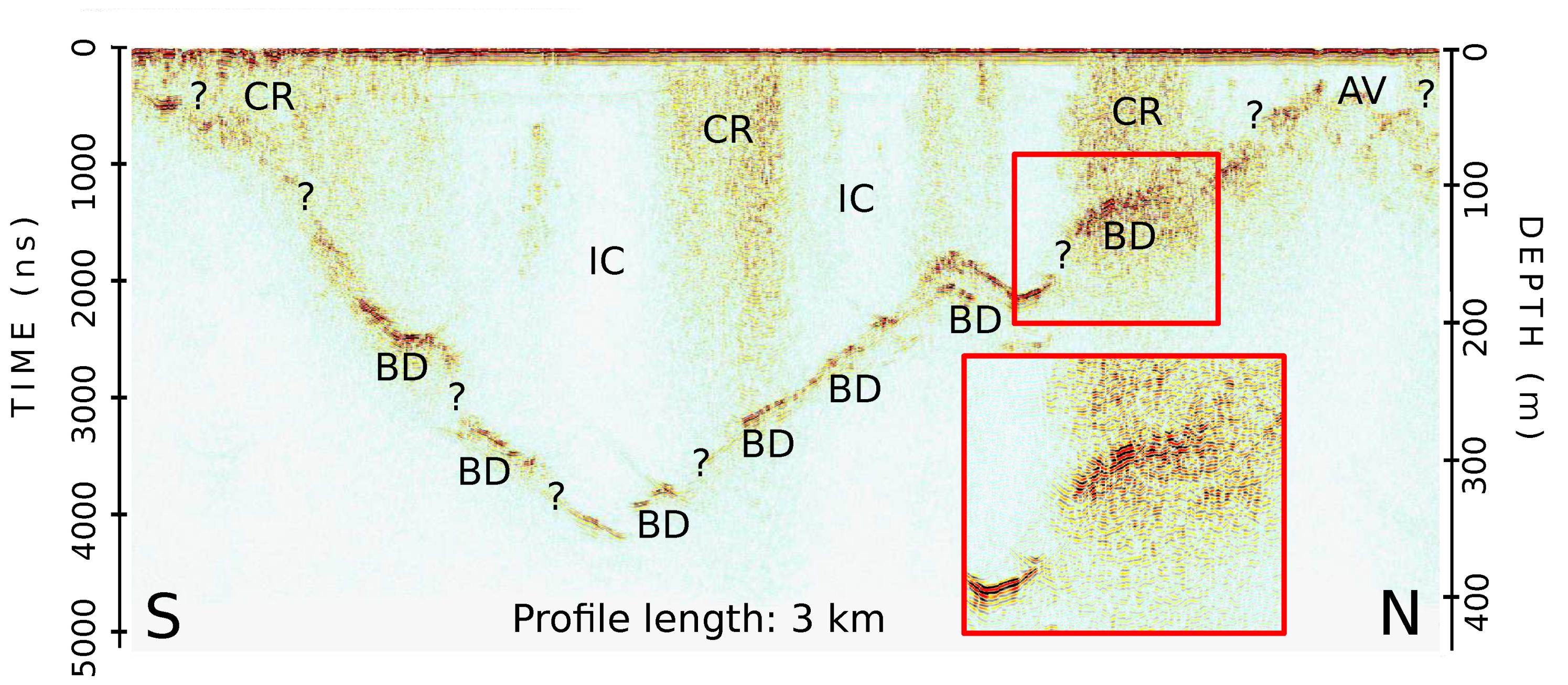
3.2. Processing of GPR Data

All data were processed with the software REFLEXW v.8.5 (Sandmeier geophysical research). The GPR collects data at a rate of 10 Hz while flying nominally at ∼20 m s 1 , corresponding to a sampling interval of ∼2 m . For one trace (time series) of 10 . 24 μ s duration (consisting of 4096 samples) the radar averages 256 measurements in order to improve the signal-to-noise ratio. In the post-processing, the external 10 Hz GNSS data are matched to the internal 1 Hz time stamps of the logger unit to provide precise georeferencing of the antenna position. Trace header coordinates are updated with the corresponding GNSS data and the traces are interpolated for a constant ( 2 m ) trace interval. Afterwards, filtering with a 10 MHz to 50 MHz bandpass to reduce e.g., high frequency radio noise and a spike removal are applied. A gain function was used to compensate for geometrical spreading and absorption by assuming a constant absorption coefficient of 0 . 02 dB m 1 typical for cold ice [29]. Surface reflections were picked manually to derive an air/ice model which was used for a 2D finite-difference migration. Finally, the travel time in ice was picked at the bedrock reflection and converted to ice thickness by applying a constant velocity of 168 m μ s 1 [29]. Because Gourdon Glacier consists mainly of solid ice formed by regelation, no correction for firn density was applied for profiles on the outlet part. In case of data from the plateau, we applied the same standard correction value for firn and snow ( + 10 m , AWI/BAS Bedmap 1 mission summary) as used in the British-Argentinian survey to ensure data comparability. For the grayscale-plots of profiles shown in this paper the surface reflection has been shifted to time zero and a Hilbert envelope was applied to enhance the amplitude contrast.

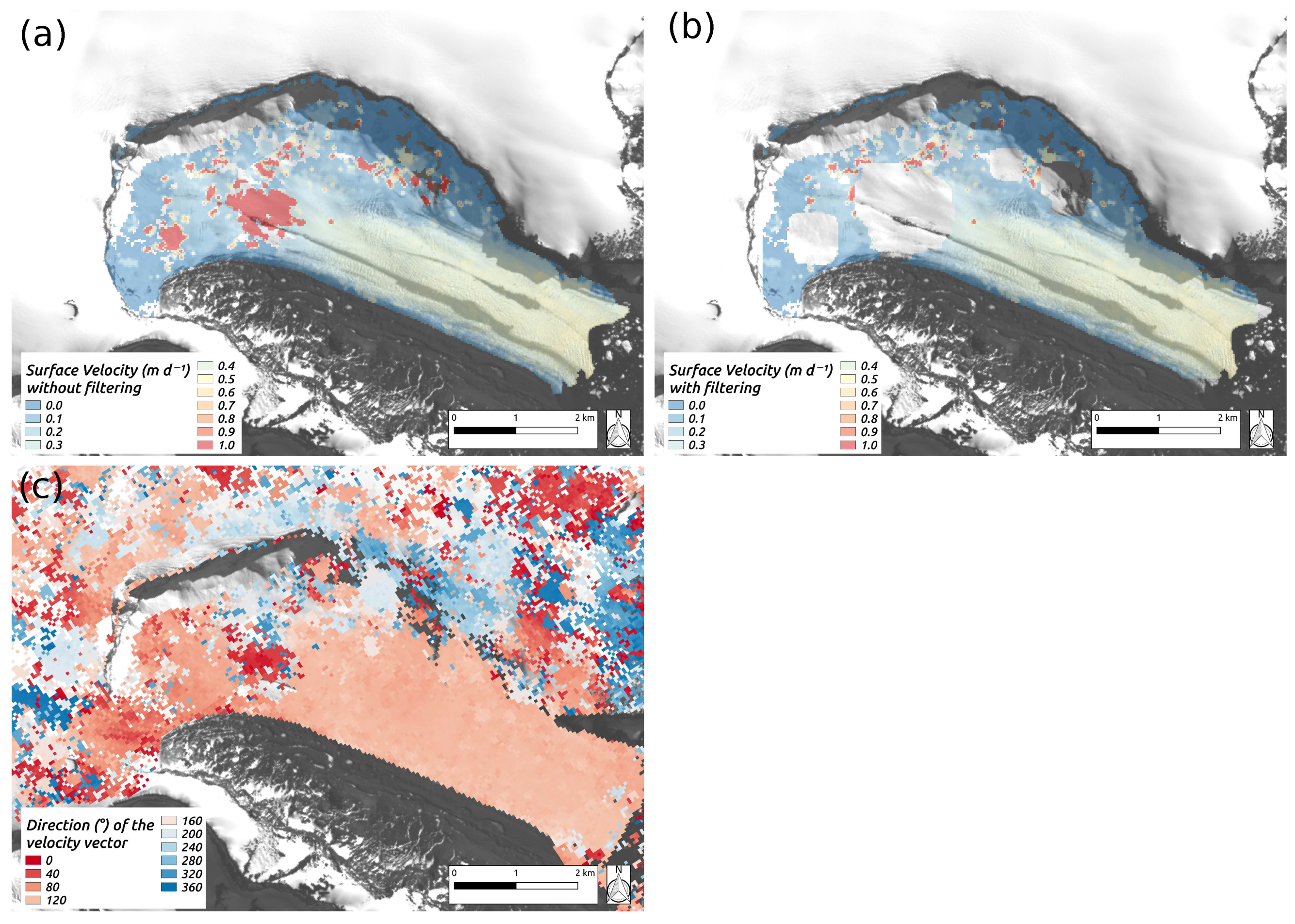
3.3. Estimation of Surface Velocities from Satellite Data

Surface velocity magnitudes and directions were calculated using synthetic aperture radar (SAR) images from TerraSAR-X and TanDEM-X satellite missions. An intensity offset tracking algorithm implemented in the GAMMA remote sensing software [30] co-registers two consecutive scenes and calculates the displacement by tracking consistent image structures like crevasses or rocks on the glacier surface. Details to the processing can be found in Seehaus et al. [31]. Furthermore, unreliable velocity estimates, mostly near to the cliff where the standard deviation in a 21 × 21 pixel moving window is larger than 0 . 5 m d 1 , were excluded [23]. Velocity maps of Gourdon Glacier are available for the period August 2014 until April 2018 (Table A1) at Pangaea doi:10.1594/PANGAEA.907062. One example is shown in (Figure A2a,b) in the Appendix A. Data gaps, which occur after the filtering, where filled along the flux gates by linear interpolation between the last available measurements. The fraction of data gaps for each flux gate and time frame can be found in Table A3.

3.4. Ice Thickness Interpolation and Reconstruction

Following Blindow et al. [32], a triangular irregular networks (TIN) method is applied for the interpolation of the spatially uneven distributed ice thickness measurements. A TIN approximates e.g., a terrain surface by a set of triangles [33]. Afterwards, a linear interpolation is applied by using the sample points within each triangle and a plane equation is fitted through the three grid points at the triangle vertices [34]. Additionally, zero ice thickness was assumed at the glacier margins except along the calving front. The calving front thickness coincides closely with a GPR profile. Thus, values were filled using nearest neighbour interpolation.
Additionally, the ice thickness is interpolated by a mass-conserving reconstruction approach (MCRA) [17]. Ice thickness was set to zero for the land-terminating margin like in case of the TIN method, while a free boundary condition was used at the calving front. In this approach, a glacier-wide flux field is inferred from the difference between the surface mass balance (SMB) and elevation changes using mass conservation. Relying on the shallow ice approximation [35], the flux field is then translated into thickness values. The necessary ice viscosity is estimated from thickness measurements. In the case of this study, no glacier elevation changes were assumed and the surface geometry was derived from the 8 m Reference Elevation Model of Antarctica [36] (imagery acquired over JRI between August 2015 and July 2016). Accumulated SMB data for the year 2017 on Gourdon Glacier were taken from the nearest grid cells in the MAR regional climate model in the version 3.9 with a spatial resolution of 7.5 km [21,22]. In Lippl et al. [23], the suitability of MAR regarding the differences between the lower lying outlet glaciers and the higher elevated plateau on JRI were evaluated by in situ measurements for different climate variables. Data revealed that for temperature, surface pressure and relative humidity, MAR is able to reflect the temporal variability at the outlet glaciers with a reasonable constant bias. Wind data were more suspicious to possible uncertainties, which holds true probably also for precipitation/SMB [23]. Interpolation approaches like the MCRA relying on mass conservation are dependent on accurate surface mass balance data [17]. The above described MCRA only considers the SMB at the outlet glacier. In case of cliff-separated, small outlets like Gourdon Glacier, the spatial resolution of MAR is not sufficient to resolve the high ablation at the frontal part correctly. Additionally to the uncertainty in the SMB data, mass input from its catchment area on the plateau is neglected in the SMB, but has to be taken into account when the outlet is considered as a own system. Therefore, the ice discharge estimate from the flux gate P2 (Figure 2a) for the GPR measurements from 2018 was included as an additional mass input. We name this model as MCRA+. The effect of the SMB between P2 and the ice cliff is negligible due to the small affected area.

3.5. Calculation of Ice Discharge

For grounded parts of the glacier, the ice discharge Φ can be calculated with the following formula as the mass flux through a given surface S approximated per area bin n (after [37]):
Φ = S ρ v d S = n ρ L n H n f v n cos α n
with the density of ice ρ , L n and H n the width and thickness of each area bin n, f the ratio of the surface to the depth-averaged velocity, v n the magnitude of surface velocity, and α n the angle between the surface velocity vector and the perpendicular line to the flux gate (in the following stated as “velocity direction”). The flux gates G1-G8 and P2 (purple lines in Figure 2a) were chosen with the intention to maximize their overlap with real GPR profiles (black lines in Figure 2a). This procedure should minimize an impact through the interpolation. The only small differences resulting from missing data near to the cliffs or non-linear flight paths can be seen by comparing the purple flux gates with the black lines. Due to the small size of data gaps at the cliff and the slow glacier velocity in this area, the effect on the overall ice discharge is assumed to be negligible. For the sake of simplicity, we state data along these flux gates in the following as “non-interpolated”.

3.6. Error Estimation

3.6.1. Ice Thickness Measurements

According to Lapazaran et al. [38], for each measurement point i the error in the ice thickness measurements ϵ H D a t a can be split into two independent error sources: the error resulting from the pulsed radar measurement ϵ H G P R , and the error in the horizontal positioning ϵ H x y at the measurement point, defined by
ϵ H D a t a i = ϵ H G P R i 2 + ϵ H x y i 2
The error resulting from the GPR measurements can be calculated by [38]
ϵ H G P R i = 1 2 τ i 2 ϵ c 2 + c 2 ϵ τ 2
with τ i the two-way travel time for each measurement point i, c the radar wave velocity, and ϵ c and ϵ τ the corresponding errors. We applied a single value of c = 168 m μ s 1 [29] for the whole glacier. Thus, according to Lapazaran et al. [38], in the areas containing firn, a value of ϵ c up to 8 . 4 m μ s 1 is possible. ϵ τ can be estimated by 1 f and is 0 . 04 μ s for the applied 25 MHz antenna when considering a constant velocity equal to 168 m μ s 1 . The uncertainty of 8 . 4 m μ s 1 for ϵ c is supposed to be too high over large areas of the outlet. However, in proximity to the cliff, the snow avalanches from the plateau can increase the uncertainty. Thus, a very conservative value was chosen. Moreover, errors due to misinterpretation of the bedrock reflectors or variations in the GNSS accuracy can arise [28]. These systematic errors are difficult to quantify due to their variability in dependence of the location on the glacier, but are described in the interpretation of observed ice thickness differences in Section 4.2 and in the Appendix A (Figure A3).
The positioning related ice thickness error ϵ H x y i can be estimated by [38]
ϵ H x y i = ϵ H x y P a r a i 2 + ϵ H x y P e r p i 2
with ϵ H x y P e r p i and ϵ H x y P a r a i the components of the ice thickness error perpendicular and along the flight track. Each component can be estimated by searching for the maximum ice thickness deviation for each i within a search radius determined by the positioning errors ϵ x y P e r p and ϵ x y P a r a . Both can be estimated with [38]
ϵ x y P e r p = ϵ x y G P S
and
ϵ x y P a r a = ϵ x y G P S 2 + ϵ Δ x y 2
ϵ x y G P S is the horizontal positioning uncertainty in the GPS measurement and ϵ Δ x y is the horizontal positioning uncertainty accounting for the movement along the flight path between two measurements.

3.6.2. Surface Velocity and Direction

The summed error σ v S U M of the derived velocities is assumed to be the square root of the quadratic sum of two independent error sources, the co-registration error ( σ v c ) and the error of the tracking algorithm ( σ v T ) (Seehaus 2015: S2). σ v c is calculated as the root-mean-square error (RMSE) of velocities measured over non-moving ground, which is not influenced by SAR layover and shadowing. The tracking error (in m d 1 ) is estimated using the following formula [39]:
σ v T = C Δ x z Δ t
where C is the uncertainty of the tracking algorithm, Δ x is the image ground range resolution, z is the oversampling factor, and Δ t is the time interval between the SAR images. We followed the approach from Seehaus et al. [31] with z = 2 , C = 0 . 2 , and Δ x = 2 . 5 m for TerraSAR-X/TanDEM-X [39]. The error estimates associated to each single combination of TerraSAR-X/TanDEM-X scene pairs are in Table A1. σ v S U M is used as Δ v i in Formula (9). More details e.g., to the location of the stable areas can be found in Lippl et al. [23]. The error in the velocity direction Δ α i is estimated similar to Sánchez-Gámez and Navarro [37] as the standard deviation of α j for j i 4 , i + 4 . In Figure A2c it is visible that the calculated directions of the velocity vector are relatively constant at the lower part of the glacier. At the upper part of the outlet glacier, difficulties in the feature tracking, e.g., due to avalanches, cause a much higher variability, resulting in higher errors for the flux gates G7 and G8.

3.6.3. Ice Discharge

Applying error propagation, the deviation in ice discharge σ Φ can be estimated using the propagated errors from the density of ice ρ , the width L, the ice thickness H, the ratio of the surface to the depth-averaged velocity f, as well as the magnitude v and direction α of the surface velocity vector by
σ Φ = ( σ Φ ρ 2 + σ Φ L 2 + σ Φ H 2 + σ Φ f 2 + σ Φ v 2 + σ Φ α 2 )
Using the rules of error propagation, for each x ρ , L , H , f , v , α ; the error σ x as the sum over all area bins n with x n ρ n , L n , H n , f n , v n , α n can be calculated by
σ x = ( n ( Φ n x n Δ x n ) 2 )
Following the approach from Sánchez-Gámez and Navarro [37], we assume L n to be free of errors, especially in the case of Gourdon Glacier. The glacier border at the northern side can be differentiated very sharply from the cliff, and the influence at the southern border can be neglected due to the measured low ice thickness values. ρ is estimated with 900 ± 17 kg m 3 for the whole glacier area. The ratio between depth-averaged and surface velocity can vary between 0 . 8 and 1 . 0 , depending on the influence from basal sliding [40]. Thus, we tested the influence on the summed error with a value of 0 . 9 and an uncertainty of ± 0 . 1 . H i , v i and α i are depending on the specific location at the glacier. Therefore, the adjacent deviations are calculated directly from the measured radar and velocity data. Δ H n is the calculated average of all errors ϵ H D a t a i for each radar measurement i within one area bin n. The spatial resolution of the velocity product is already 10 m such as the step size n. Thus, Δ v n = Δ v i is the error in velocity magnitude, whereas Δ α n = Δ α i is the error in velocity direction. The calculation of both is described in Section 3.6.2.

4. Results

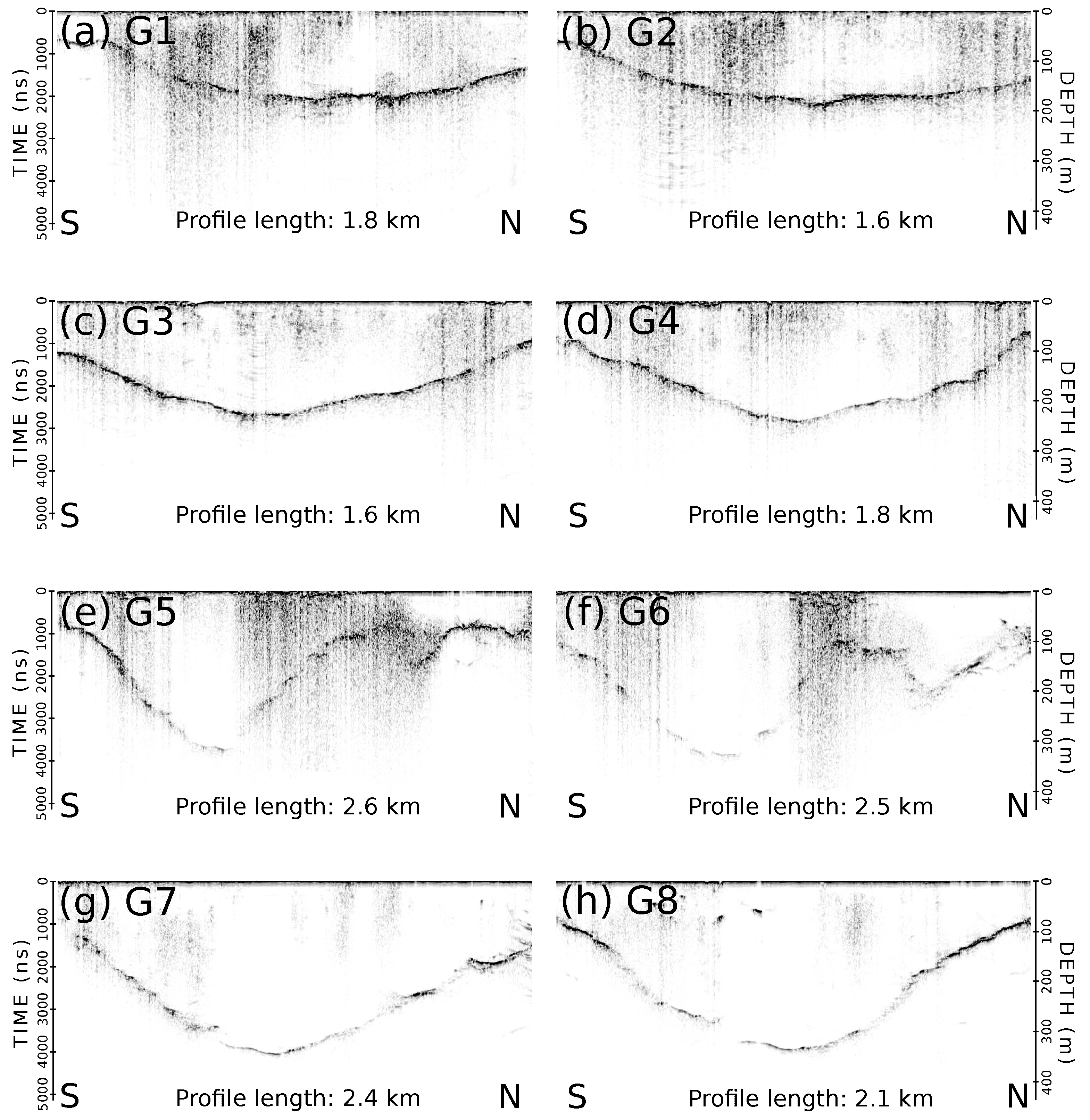
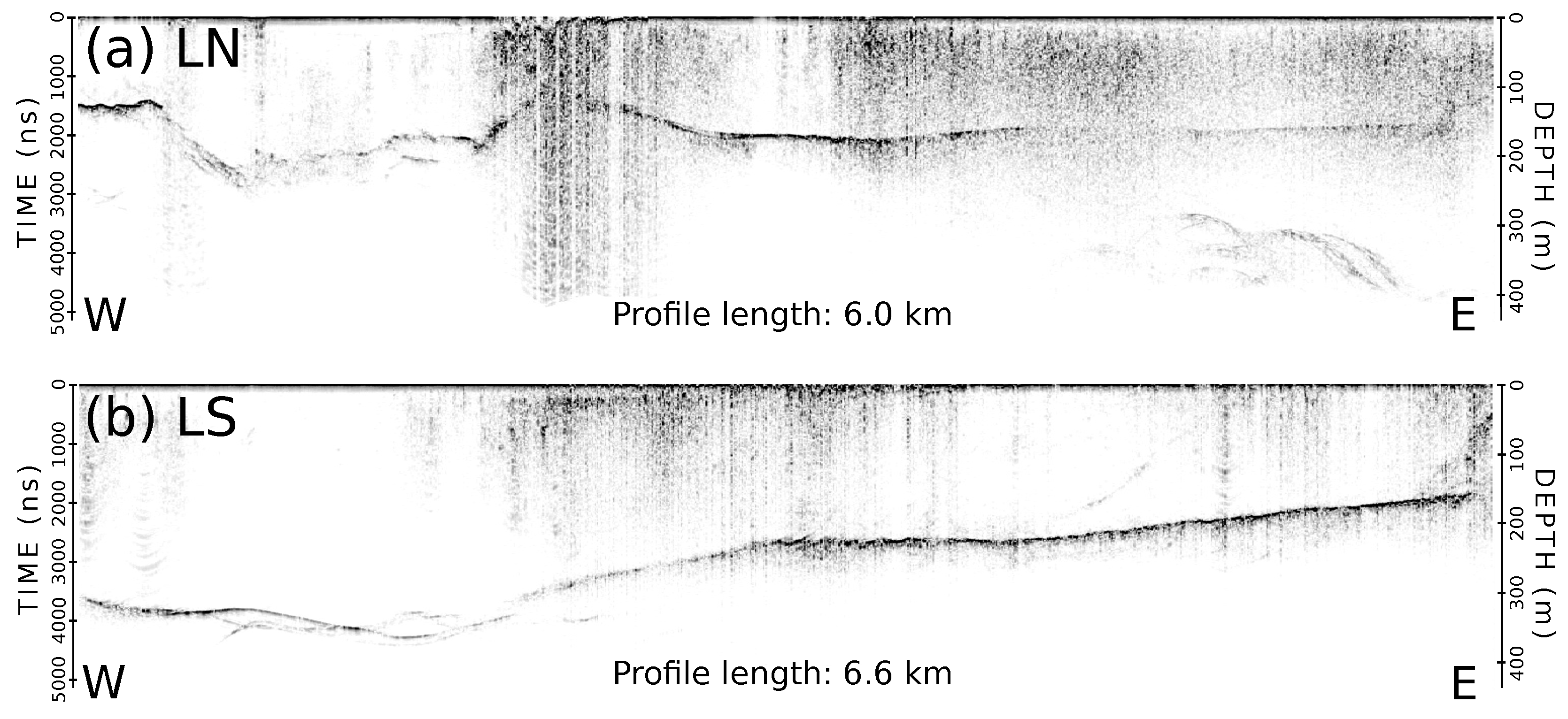
4.1. Report of Ice Thickness Measurements

The ice thickness measurements from the GPR campaign in 2018 are shown in Figure 2a and the measurements from 2017 in the subset Figure 2b. The overall maximum ice thickness is observed at the measurements on the most upper part of the plateau with values of more than 400 m . In the lower part of the catchment area on the plateau the ice thickness shows high lateral variations, which slightly decreases in proximity to the cliff at flux gate P2. The ice thickness measurements on the outlet part of Gourdon Glacier are showing a smooth pattern with the largest ice thickness ∼3 km south-east from the ice cliff. In this area, the bedrock is below sea-level.
In order to investigate if ice discharge variability is resulting from short-distance ice thickness variations, we compare two adjacent radar profiles (G1 and G2, G3 and G4, G5 and G6, G7 and G8, Figure 3). No larger differences are found between the ice thickness profiles on the left of Figure 3 compared with their counterpart on the right. Ice thickness measurements at the flux gates G1 and G2 are ranging from ∼60 m at the southern moraine up to ∼170 m for G1 and 180 m for G2 close to the middle of the glacier bed. Ice thickness at the northern end is still larger than ∼110 m , but it has to be considered that measurements with a distance smaller than ∼500 m to the cliff were not possible. The largest ice thickness values of ∼220 m or ∼230 m are reached for G3 and G4. Data from G5 and G6 are showing a structural bump within the glacier (shortly after the middle of the profile) with ice thickness values lower than 100 m , before a second depression occurs more to the north. The ice over the bump is strongly affected by crevasses hampering the detection of the bedrock signal in the GPR profiles. This is also the case in the southern parts of G1 and G2, but not as strong that bedrock detection is not doable anymore. Largest ice thickness values for G5 (∼305 m ) and G6 (∼315 m ) are almost at the same level than for G7 (∼330 m ) and G8 (∼320 m ). Further radar measurements indicate that the glacier reaches its thickest point between G6 and G7, slightly shifted to the south of the glacier center.
In Figure 4, the northern (LN) and southern (LS) longitudinal GPR profiles (Figure 2a) are shown. The bump observed in the transverse profiles is also visible in the northern longitudinal profile ∼2 km from the western cliff margin. The different length scale has to be considered for comparisons with the cross profiles. Additionally to a blurring of backscatter in regions with more crevasses, a clear second backscatter profile is visible for the last 1 km 1 . 5 km before the frontal margin of the northern profile. The reason is probably backscattering from the side walls, but it can be clearly distinguished from the true bedrock.
On the plateau of JRI two profiles P1 and P2 were acquired (Figure 5). The location with the highest ice thickness of ∼400 m is found just outside of Gourdon Glaciers’ catchment area (Figure 2a). About 800 m to the north-east, our measurements in 2018 observed an ice thickness of more than 400 m . However, ice thickness at the catchment boundary of Gourdon Glacier is not more than 290 m . The ice thickness in profile P2, also used as a flux gate for the estimation of ice discharge from the plateau, shows variability along the cliff. Whereas ice thickness along the first part at the eastern corner is almost zero, ice thickness varies mostly between ∼100 m and ∼160 m . There are several major bedrock depressions in the profile P2. The ice thickness at the deepest depression at the southern end of the profile reaches ∼210 m . In immediate proximity to the southern end, the ice thickness reaches zero, corresponding to the bedrock outcrop observable in the background Landsat image (red arrow in Figure 2a). The topography in the radargram with the depression in the middle (Figure 5, arrow 1) looks like a caldera, a remnant of the volcanic history of JRI.

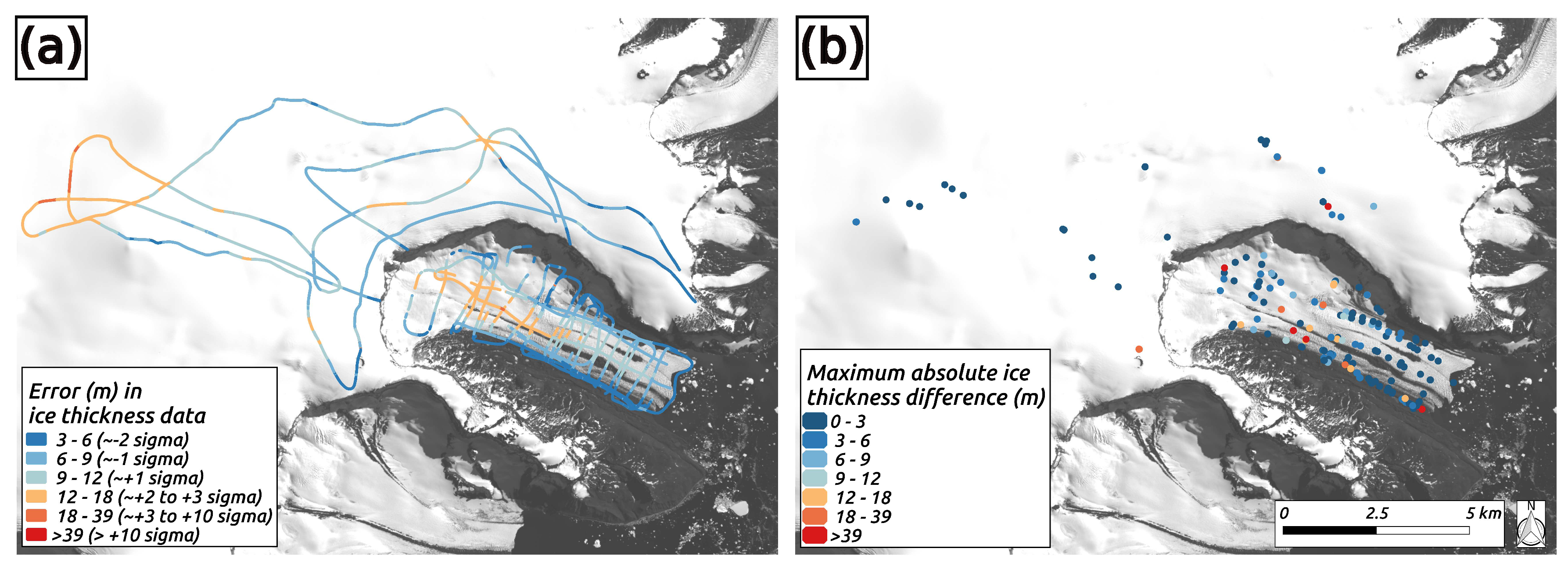
4.2. Error Estimation for Ice Thickness Measurements

Applying Formula (3) with the observed travel times at each measurement point i for the measurements from 2018, we get ϵ H G P R i between 3 . 62 m and 18 . 08 m for the outlet part of Gourdon Glacier. The mean of all measurement points is 8 . 30 m with a standard deviation of 3 . 36 m . At the plateau, values range between 3 . 37 m and 20 . 21 m (Mean: 9 . 50 m , Std: 3 . 01 m ). Considering an average helicopter velocity of 27 m s 1 and a GNSS sampling interval of 10 Hz , ϵ Δ x y is 2.7 m. Together with a horizontal uncertainty of ϵ x y G P S = 0 . 08 m in the GNSS measurements, this results in ϵ x y P e r p = 0 . 08 m and ϵ x y P a r a = 2 . 70 m by applying Formulas (5) and (6). Due to the low error in the GNSS measurements, ϵ x y P e r p can be neglected. By searching for the maximum deviation in ice thickness along track, ϵ H x y = 0 . 49 m is observed in average for the outlet part. The average deviation within a 2 . 70 m radius on the plateau is ϵ H x y = 0 . 29 m . Taking ϵ H x y for each i in Formula (2) implicates in summary an average error of ϵ H D a t a = 8 . 36 m .
In case of the plateau, the mean ϵ H D a t a is 9 . 53 m . Due to stronger velocity variations of the helicopter on the plateau, the maximal deviation in ice thickness was calculated also within a search radius of 5 m (according to a maximum velocity of 50 m s 1 ) and revealed an average of ϵ H x y = 0 . 42 m . However, the overall error ϵ H D a t a is as well dominated by ϵ H G P R . The final ice thickness error for each data point is shown in Figure 6a.
The error in the ice thickness measurements is in general below 20 m (Figure 6a), with the highest values in the areas of the largest ice thickness at the upper catchment of the outlet part and the western part on the plateau. In most of the other areas, the error is between 6 m and 12 m .
In order to assess ice thickness differences introduced by the different flight directions, the search radius of 2 . 70 m was applied also for the estimation of the maximum absolute ice thickness difference at crossing flight paths in Figure 6b. For Gourdon Glacier the average deviation is 5 . 74 m , for the plateau it is 12 . 88 m . However, the higher average deviation at the plateau can be explained by the low amount of data and the higher influence from single outliers, but also the overall higher ice thickness values causing an increase of the uncertainty. Within the outlet part there is a slightly higher average deviation of 6 . 93 m for all values above the flux gate I2 (Figure 2a) in comparison to 5 . 11 m below of I2. Outliers with ice thickness differences of more than 40 m are observed e.g., in immediate proximity to the cliff and strongly crevassed areas. Especially these regions can suffer from higher errors in case of a misinterpretation of the bedrock backscatter. We visualize these potential problems in Figure A3 in the Appendix A.

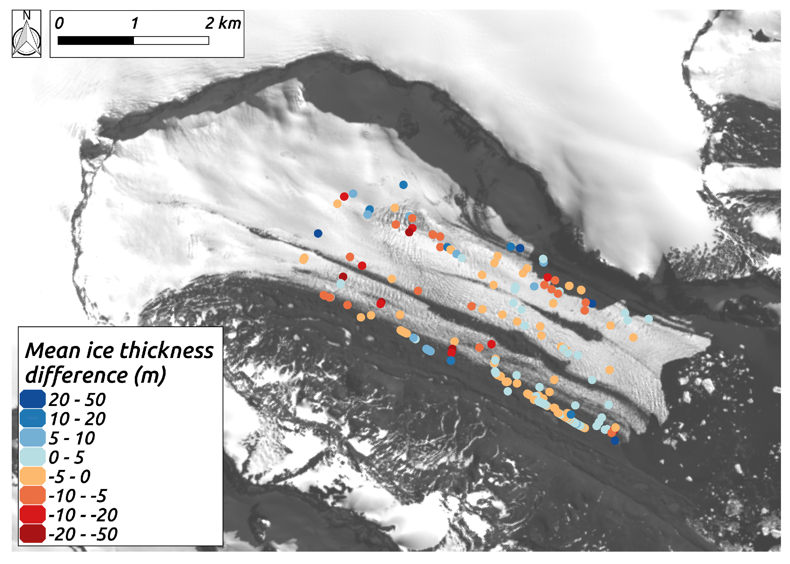
4.3. Comparison with Data from 2017

For the comparison of the ice thickness data from 2018 with the measurements from 2017, a search radius of 2 . 7 m was applied (according to the position accuracy ϵ Δ x y , resulting in 860 intersects). In Figure 7, the average absolute deviation between the GPR measurements of the different years is 4 . 10 m , which sums up to a decrease by 0 . 39 m when considering the sign of the deviation. Both values are smaller than the error of ϵ H D a t a = 8 . 36 m . Outliers with higher deviations at the upper parts could be influenced by a higher amount of thicker ice, but also by a stronger influence from differences due to ice avalanches. No further spatial pattern of ice thickness differences between the two years can be observed.

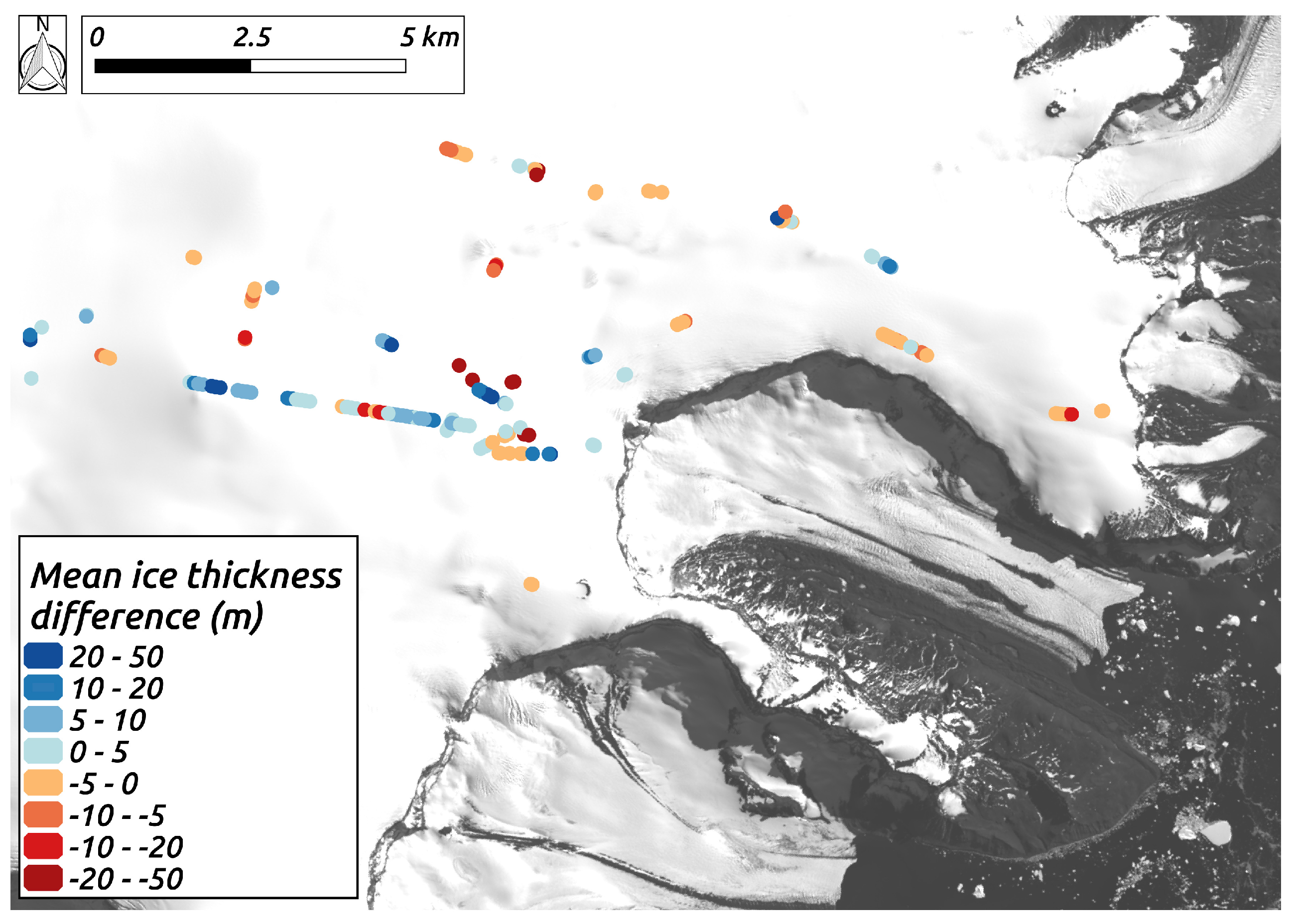
4.4. Comparison with Data from 1995–1998

The measurements on the plateau from 2018 of this study were compared with data from the British-Argentinian missions in the years 1995/96 and 1997/98. Besides their specified uncertainty in ice thickness of 10 m , differences in the along track discretization intervals hamper a comparison with our dataset. The search radius for intersecting points had to be increased to at least 10 m (31 intersects) where an average absolute deviation of 7 . 11 m and an average thinning of 0 . 35 m is observed. By applying a search radius of 100 m (331 intersects), the average in absolute deviation is 8 . 33 m , for a search radius of 50 m (174 intersects, Figure 8) we obtained an average absolute deviation of 8 . 00 m .

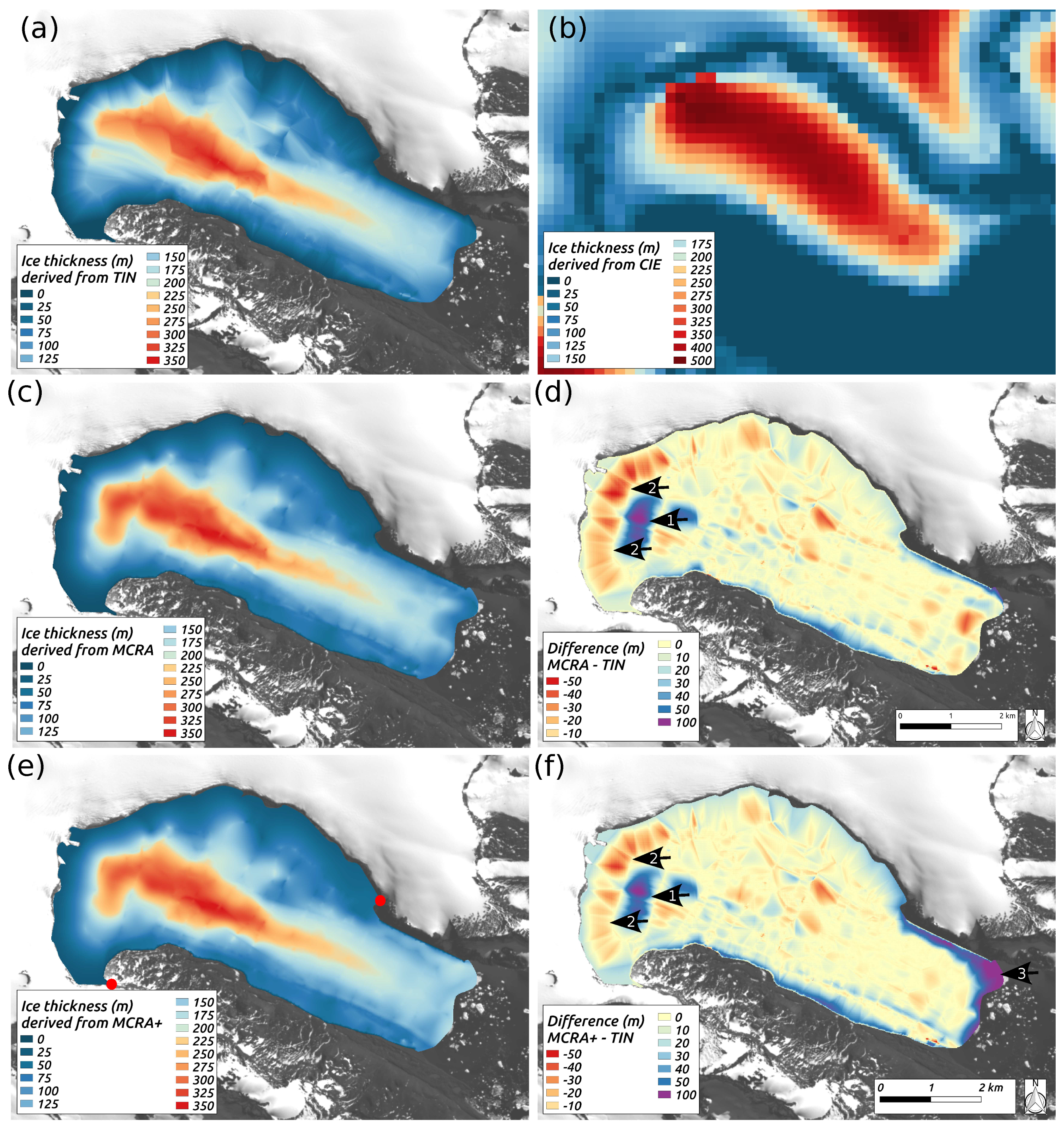
4.5. Interpolation and Reconstruction

Figure 9 illustrates the interpolated or reconstructed ice thickness data from the GPR measurements from 2018 applying the TIN method (Figure 9a), the MCRA (Figure 9c), and the MCRA+ (Figure 9e). Ice thickness simulated by the CIE [19] from the models participating in ITMIX [4] is presented in Figure 9b. The CIE at Gourdon Glacier does not rely on field data and only uses interpolated surface and bedrock elevation data.
The mean difference between the results from the MCRA and the TIN method is 3 . 70 m (Figure 9d). The area with higher ice thickness values larger than 200 m elongates slightly further to the western end of the glacier in the MCRA, resulting in strong positive differences up to 70–80 m (Figure 9d, Arrow 1). Directly at the border to the cliff, the ice thickness is slightly higher for the MCRA at most parts of the glacier (∼10–20 m ). However, between the larger maximum ice thickness values (Figure 9d, Arrow 1) and the larger ice thickness directly at the western cliff, the thickness is lower in the MCRA (up to 50 m in Figure 9d, Arrows 2) than in the approach using the TIN. In general, the results from the MCRA (Figure 9c) appear more smoothed, whereas the results from the TIN (Figure 9a) show more variability resulting from the interpolation between the measurements along the GPR flight paths. Throughout the nearly complete glacier outlet the ice thickness from the CIE is more than 300 m , introducing a large error for the outlet part of Gourdon Glacier. Moreover, the maximum ice thickness is over-estimated by ∼100 m . The impact on ice discharge estimates will be assessed in the next section.
The interpolated ice thickness from the MCRA+ is shown in Figure 9e. An annual mass input of 77 Mt (Cumulated ice discharge in 2017 from Figure 10) was distributed equally along the ice cliff between the two red dots and used as a mass-input boundary condition in the reconstruction approach. Considering the difference between the MCRA+ and the TIN (Figure 9f), increased values (∼10 m higher than in the MCRA without the additional mass input) can be observed near the ice cliff. Toward the center of the glacier (Figure 9f, Arrows 2), the negative differences in the MCRA (in comparison to the TIN) can be compensated by the additional mass input along the cliff using the MCRA+. Higher differences to the TIN are introduced by the larger ice thickness at the glacier front for the MCRA+ (up to 100 m ), especially at the northern part (Arrow 3). It can be expected that the model approach adds two much additional mass input at the northern cliff boundary of the frontal part, resulting in an overall increase of the mean difference between the MCRA+ and the TIN ( 8 . 49 m in comparison to 3 . 70 m for the MCRA).

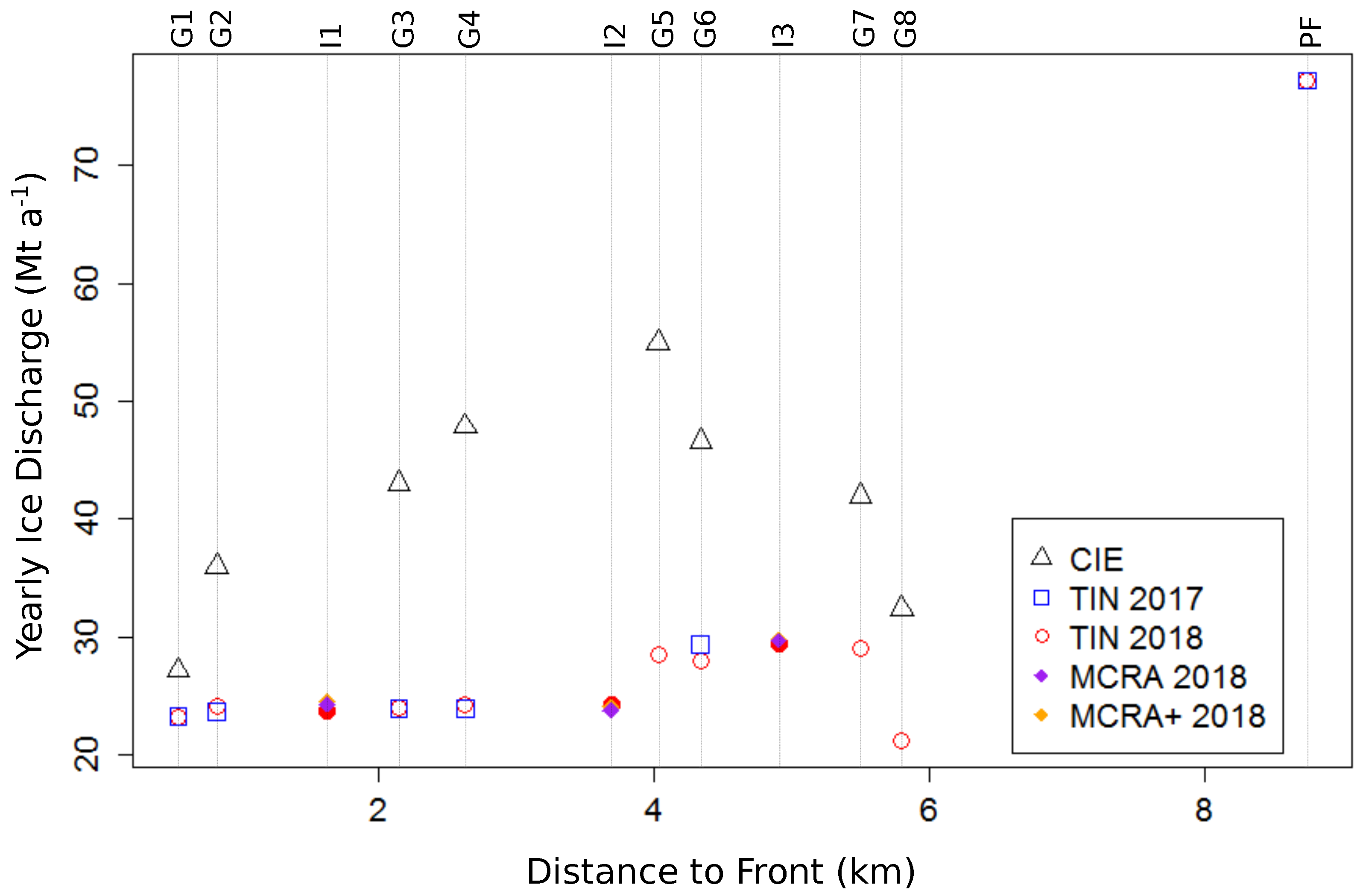
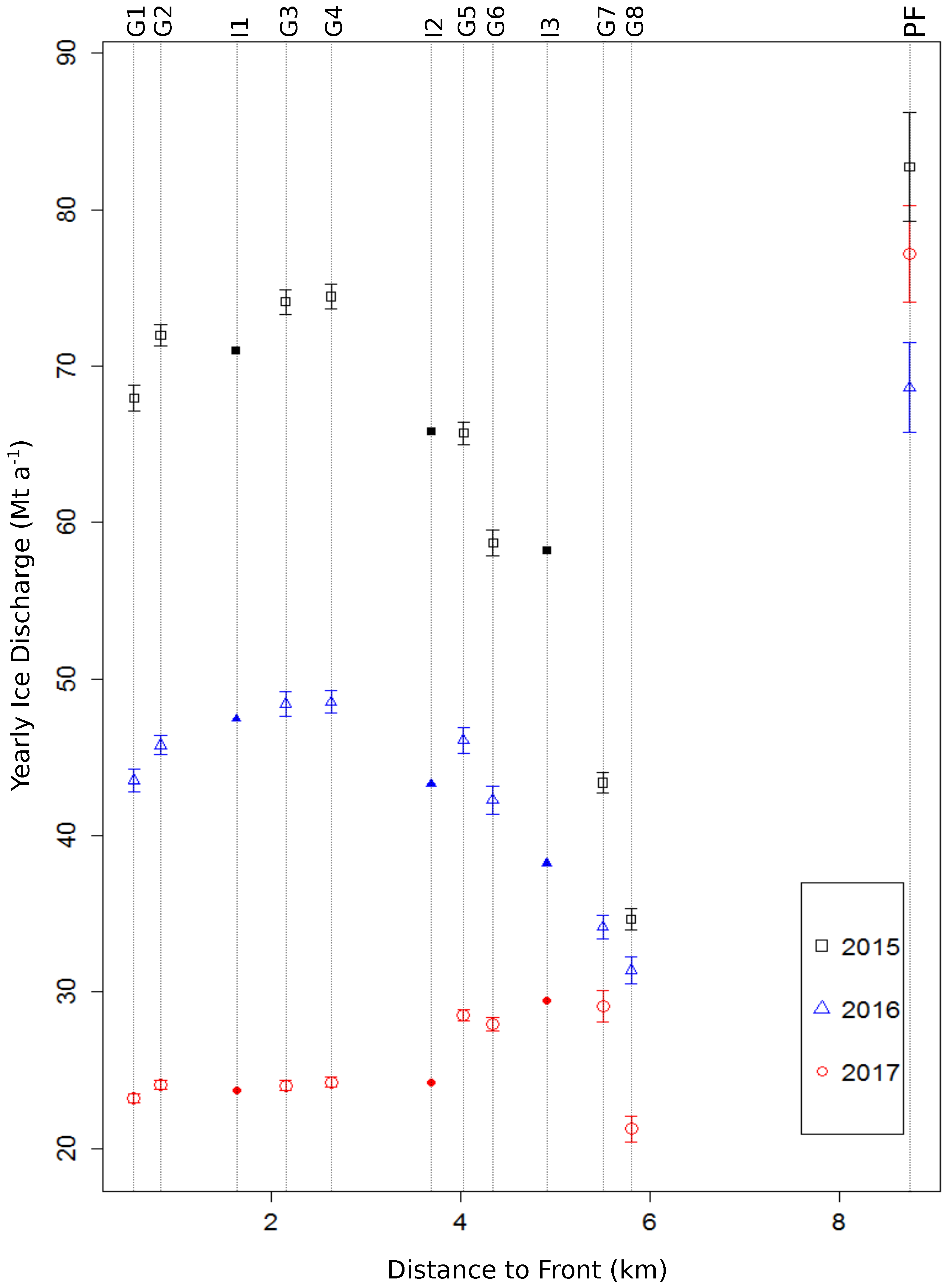
4.6. Estimation of Ice Discharge

The flux gates G1-G8 and I1-I3 on Gourdon Glacier as well as P2 on the plateau shown in Figure 2a were used for the estimation of ice discharge. Three different ice thickness datasets were applied for the calculation of ice discharge along G1-G8: Firstly, the ice thickness dataset generated by the TIN interpolation from the 2018 GPR measurements (TIN 2018). Secondly, we used a TIN-interpolated ice thickness from 2017 (TIN 2017) where possible (flux gates G1–G4, G6) to evaluate differences introduced by variations in ice thickness. Third, the simulated data from the CIE are applied to assess the difference in ice discharge by using observational unconstrained ice thickness values. To evaluate the influence from the different interpolation/reconstruction methods, the ice discharge is calculated additionally along the flux gates I1–I3 where all ice thickness measurements are interpolated. Additionally to the TIN interpolation from the 2018 GPR measurements we did the flux analysis for the MCRA (MCRA 2018) and the MCRA+ (MCRA+ 2018) products.
The resulting ice discharge for the time frame 1 January 2017 until 31 December 2017 is shown in Figure 10 for the different flux gates ordered by their distance from the glacier front. The estimated surface velocities from the TerraSAR-X scene pairs within this time step were used and weighted according their proportional amount of days. Results using the ice thickness from the 2017 and from the 2018 GPR measurements show only slightly differences for G6, whereas the ice discharge for the flux gates G1–G4 is almost the same in both cases. The ice discharge from the simulated CIE data is much higher. The difference to the TIN 2018 is minimal 4 Mt a 1 in case of G1, but reaches much higher values for the upper located flux gates with a maximum of ∼30 Mt a 1 for G5. Ice discharge from the interpolated data (I1–I3) using the TIN 2018 method and for both the MCRA 2018 and the MCRA+ 2018 datasets are fitting very well to the results from the flux gates along in situ data.
In Figure 11, the yearly ice discharge calculated with the TIN interpolation from the 2018 GPR measurements is shown for the years 2015, 2016, and 2017. The associated error estimates are calculated using Formulas (8) and (9) with the ice thickness data from 2018. Thus, the error is calculated only for the flux gates G1–G8 and PF where a correct error estimation in ice thickness without a considerable impact from the interpolation is possible. The estimated ice discharge can be biased by changes in ice thickness between the different years which we were not able to observe. However, we assume that these changes are within the estimates errors of ice thickness measurements in Section 4.2. In 2016 the ice discharge is about twice the value of 2017, and in 2015 the threefold. This is mostly due to the higher glacier velocities. The ice discharge pattern described for the velocity estimates from 2017 with increasing discharge from G1 to G6 and a decrease for G8 is different in 2015 and 2016. In these years, the highest discharge is reached closer to the glacier front at flux gate G4. A constant decrease is observed for the upper located flux gates. In 2017 the calculated errors are very low with values ∼0.2–0.3 Mt a 1 , especially for G1–G6. In 2015 and 2016 the errors for the lower flux gates are ∼1 Mt a 1 . The ice discharge from the plateau at flux gate PF is between 68 Mt a 1 and 83 Mt a 1 for the different years. An error of ∼3 Mt a 1 is the case for the ice discharge from the plateau in all three years.
In Table 1, error estimates split into each single parameter (except σ Φ L which is neglected) of Formula (8) are presented for the flux gates. In the following we focus on the values for G1 and G8 as the two most contrary flux gates. For both flux gates the lowest source of error is normally the density in ice ( σ ρ ), followed by the error in ice thickness ( σ H ), where the error accounts between 0 . 09 Mt a 1 and 0 . 26 Mt a 1 .
For G1 with more reliable velocity data, the error in the ratio between surface and depth-averaged velocity ( σ f ) is often the largest source of error, with a value about the double of σ H . The error from the velocity magnitude ( σ v ) is in the same range like σ f in 2016 and 2017, and less in 2015. The yearly error in the velocity direction ( σ α ) in 2017 is very low with 0 . 011 Mt a 1 , but in the same range like the other error sources in 2015 and 2016 with values ∼0.3 Mt a 1 .
For G8, σ v is only about the half of σ f in 2015, but about the double in 2016. σ α does not show exactly the same pattern as σ v . The yearly error in σ v is between 0 . 50 Mt a 1 and 0 . 71 Mt a 1 and the highest source of error in all three years.
Due to the reason that the ice thickness of the GPR measurements from 2017 is similar to the values for 2018, we resign a specific error calculation for the radar measurements from 2017. The unknown error in ice thickness for the CIE data is surely much higher, influencing the overall higher ice discharge estimates for all flux gates. The ice discharge estimates for 2017 are mostly in the same range like the values for 2018. The higher uncertainty from the upper located flux gates such as for G8 can be a result from the higher amount of no-data values (Table A3) which additionally introduced uncertainty.

5. Discussion

5.1. Ice Thickness Measurements

The in situ GPR measurements revealed a variability in ice thickness between the plateau of JRI and the outlet part of Gourdon Glacier, which is not resolved in large-scale simulated CIE data. The mass input from the plateau by ice avalanches creates a strong gravitational force on the catchment area of the outlet part. In this area, the glacier starts to deepen its glacier bed, with the largest ice thickness at a distance of ∼3 km from the cliff margin. At the deepest point the glacier bed lies below sea-level.
Ice thickness differences in the comparison with the 2018 GPR measurements at crossing flight paths are mostly smaller than 3 m for the frontal part of the outlet. This implies that at least in this area a bias within one flight campaign is unlikely. The mean absolute differences of ∼7–8 m of the datasets from 1995–1998 and ∼4 m for 2017 in regard to the ice thickness from 2018 are too low to detect any temporal changes when considering the errors in ice thickness.
However, both the in situ ice thickness measurements from 2017 and 2018 are much lower than the ice thickness simulated by the CIE [4]. Beside of an over-estimation of the maximum ice thickness of ∼100 m , the over-estimation extends also to the outer and frontal parts of the glacier into regions normally applied as flux gates in glacier mass balance estimates.

5.2. Ice Thickness Interpolation

Stronger differences between the interpolation and reconstruction methods TIN, MCRA, and MCRA+ are visible especially in the upper part of the glacier outlet, where in situ measurements are rare, and at the outlet glacier boundaries. In the TIN method the latter one occurs mainly due to the introduced boundary condition of zero ice thickness at the cliff, which probably does not reflect the reality, due to relevant mass input by avalanches. The MCRA uses the same boundary condition, but simulates slight higher ice thickness values than the TIN in the direct proximity of the internal western cliff-boundary (∼10–20 m ), followed by a reversal to negative differences (up to 50 m , Arrows 2 in Figure 9d) and to positive differences (up to 100 m , Arrow 1 in Figure 9d) within a distance of only ∼1 km . The reason of this effect could be related to differences in the generation of the interpolated data between the TIN method and the MCRA. Whereas the TIN method relies on a linear interpolation between the available in situ measurements, the MCRA tries to model the underlying physical principles in glacier ice dynamic by varying the viscosity of the ice in dependence of the mass input from the SMB. However, the MCRA is “re-fitted” to in situ measurements when available again. In the case of the rare measurements at the upper part of the outlet, this could introduce the above described differences in ice thickness. Moreover, if the modeled SMB does not reflect the real conditions on the glacier outlet (which is very likely due to the abrupt elevation changes at the cliff and the resolution of 7 . 5 km in the MAR SMB data), the MCRA will pass on this bias to the reconstructed ice thickness data.
The negative differences (Arrows 2 in Figure 9d,f) can be decreased by including the additional mass input from the plateau in the MCRA+, resulting in even larger ice thickness values directly at the cliff. Nevertheless, the abrupt changes between the negative and positive deviations to the TIN method are still existing. The additional mass input in the MCRA+ is introduced only at the glacier boundaries, but due to the high cliff the influence of the avalanches could extend further to the interior of the glacier.
Directionality artefacts occur in the interpolation along the flight paths (Figure 9a). These artefacts are smaller in the MCRA approaches (Figure 9c), and can potentially be improved in the interpolation by a kriging approach with a larger or even variable search space to consider the distinct sampling interval along and across the glacier flow direction.

5.3. Ice Discharge

The overestimated ice thickness at large areas of Gourdon Glacier’s outlet in the CIE (Figure 9b) lead to an ice discharge twice to threefold the values from the TIN 2018 dataset (Figure 10). Adding the additional mass input from the plateau in the MCRA+ 2018 dataset has no effect on the ice discharge at the flux gates I1–I3. This implies that the effect of the larger ice thickness at the northern border at the front is negligible due to the slow movement of the glacier in this area. Data from MCRA 2018 and MCRA+ 2018 at the flux gates I1–I3 over interpolated data fit to the ice discharge from TIN 2018. This implicates that the interpolation using both the TIN method and the MCRA is producing an accurate estimate of ice discharge. In the case of the MCRA it has to be considered that ice thickness is calibrated to each available in situ measurement. Thus, in case of large in situ data gaps such as in the upper part of the glacier outlet, artefacts can occur when input parameters such as the SMB do not reflect the reality. The underlying glacier geometry could force errors in the SMB and therefore also in the simulated ice thickness data. This could be the case in the CIE where no in situ measurements are used for calibration.
All different data sources show the same dependence of ice discharge on the distance from the glacier front. This implicates that differences in ice thickness are supposed to have a lower impact on ice discharge than the glacier velocity. Moreover, the small differences between the interpolation using the ice thickness from the 2017 and these from the 2018 GPR measurements supports the hypothesis from the error estimates (Table 1), that the summed discharge error is mainly affected by the velocity magnitude and the velocity direction measurements. Difficult conditions for the applied intensity feature tracking algorithm due to avalanche input and melting conditions hamper the estimation of surface velocities. This results in a high amount of no-data values (especially for the flux gates G7 and G8, Table A3), but also a higher variability of measurements near to the cliff.
Considering the ice discharge at the glacier front in the year 2017 with values ∼23–25 Mt , the ice discharge from the plateau with values larger than 68 Mt in all three years seem unlikely high. However, in 2015 the ice discharge was higher with values ∼70 Mt also for the lower located flux gates. Thus, the high discharge from the plateau could be reasonable, implying the accumulation of mass at the upper part of the glacier outlet. This mass input would be transported further down in the following years as a kind of wave that passes through the glacier. The higher velocities in 2015 can be a previous wave, whereas a further acceleration would be expected after the lower velocities in 2016 and 2017. However, the acceleration could skip the upper located flux gates if the mass input was already transported further down the glacier by the avalanches.

6. Conclusions

This study has reported in situ GPR ice thickness measurements at the outlet and the plateau area of Gourdon Glacier in consideration of the internal ice cliff. A detailed error estimation of ice thickness data and their propagated error into ice discharge was given. Ice thickness from 2018 was compared with measurements from 2017 and 1995–1998, but the observed differences are within the error bars of ∼8-10 m , hampering any predictions on changes between the different time steps. Ice thickness over the outlet area was interpolated with a triangular irregular networks method and a mass-conserving reconstruction approach [17] without and with additional mass input from the plateau. Results were compared with simulated data from the CIE [4] which show a large over-estimation of ice thickness over most parts of the outlet area. This over-estimation is propagated into the estimation of ice discharge with values the twice or threefold of the values using in situ ice thickness. Differences in ice thickness using the triangular irregular networks interpolation or both mass reconstruction approaches do not have a strong impact on the estimated ice discharge in this study. However, a good coverage of in situ measurements in the area of the flux gates is required in this case. Moreover, differences in ice thickness occurred mostly on the glacier outlet margins where a slow glacier velocity diminishes their impact on the ice discharge. The importance of the accuracy of the velocity estimates is underlined by the results from the error estimation. An increase in the error of ice discharge is observed for the time frames with higher velocities (2015 and 2016), but at the upper outlet part also in 2017 with slow velocities. In the case of the latter one, the higher uncertainty results mainly from the error in the direction of the velocity vector. Moreover, the consideration of temporal variations in glacier velocity is very important due to their large influence on the error in ice discharge.
To prevent wrong ice discharge estimations e.g., for projections of sea-level rise, the usability of simulated data has to be ensured. This is necessary especially for specific glacier types such as the cliff-separated glacier in this study, which are common at the Antarctic Peninsula. In the case of Gourdon Glacier, depending on the location of the flux gate, the ice discharge by using the CIE data [4] is over-estimated by up to ∼30 Mt a 1 . Farinotti et al. [4] proposed to consider in situ ice thickness measurements at the same level like glacier outlines or surface elevation models to improve the consistency and completeness of global datasets as well as the reliability of regional-scale estimates. The results of this study have shown that the bedrock topography can be highly variable, and dedicated campaigns in data-scarce regions with a small sampling interval are required. Moreover, we propose a comparison of more in situ measurements with simulated ice thickness from projects such as ITMIX [18] with the aim to investigate potential biases and to decrease the uncertainties in glacier mass balance and sea-level rise estimates.

Author Contributions

Conceptualization, S.L. and M.H.B.; Formal analysis, S.L. and N.B.; Funding acquisition, M.H.B.; Investigation, S.L., N.B., S.M., T.C.S. and M.H.B.; Methodology, S.L., N.B., J.J.F. and T.C.S.; Project administration, S.M. and M.H.B.; Software, S.L., J.J.F. and T.C.S.; Supervision, M.H.B.; Visualization, S.L.; Writing—original draft, S.L.; and Writing—review and editing, S.L., N.B., J.J.F., S.M., T.C.S. and M.H.B. All authors have read and agreed to the published version of the manuscript.

Funding

This study was funded by the Deutsche Forschungsgemeinschaft (DFG) under the grants BR 2105/13-1 as well as BR 2105/9-1. Latter formed part of the DFG priority programme “Antarctic Research with comparative investigations in Arctic ice areas”. We would like to thank the HGF Alliance “Remote Sensing of Earth System Dynamics” for additional support. TS was financially supported by the DLR/BMWi grant GEKKO (50EE1544). Costs covered by our Argentinian partner were funded by the project from ’Balance de masa y dinámica de glaciares en la Península Antártica’ from Instituto Antártico Argentino. Access to satellite data was kindly provided by various space agencies, e.g., under ESA AO 4032, DLR TerraSAR-X Background Mission Antarctic Peninsula and Ice Shelves, TSX AO LAN0013, TanDEM-X Mission TDX AO XTI_GLAC0264, ASF, and GLIMS as well as NASA and USGS.

Conflicts of Interest

The authors declare no conflict of interest. The funders had no role in the design of the study; in the collection, analyses, or interpretation of data; in the writing of the manuscript, or in the decision to publish the results.

Abbreviations

The following abbreviations are used in this manuscript:
CIEconsensus ice thickness estimate
GNSSGlobal Navigation Satellite System
GPRground penetrating radar
GPSGlobal Positioning System (in the context of this paper single frequency GPS measurements)
ITMIXIce Thickness Models Intercomparison eXperiment
JRIJames Ross Island
MARModèle Atmosphérique Régional
MCRAmass-conserving reconstruction approach
MCRA+mass-conserving reconstruction approach with additional mass input from the plateau
RGIRandolph Glacier Inventory
RMSEroot-mean-square error
SARsynthetic aperture radar
SMBsurface mass balance
TINtriangular irregular networks

Appendix A

Figure A1. (a) The GPR antenna flown as a sling load by a Bell 212 helicopter. (b) Detailed view of the GPR antenna system. (c) The frontal part of Gourdon Glacier with the northern cliff boundary, photographed from the southern moraine.
Geosciences 10 00012 g0a1
Table A1. Satellite scenes used as slave and master image in intensity feature tracking with aquisition dates, path and orbit informations, as well as the associated error estimates in m d 1 . σ v T is the error of the tracking algorithm, σ v C the co-registration error, and  σ v S U M the square root of the quadratic sum of both [23].
Sensor Scene 1PathDate Scene 1Abs. Orbit Scene 1Date Scene 2Abs. Orbit Scene 2Time Step (days) σ v T
(m d 1 )
σ v C
(m d 1 )
σ v SUM
(m d 1 )
TSX0140-01413 August 201422,9897 October 201423,824550.0050.0090.010
TDX0140-0147 October 201423,82429 October 201424,158220.0110.0140.018
TDX0140-01429 October 201424,1581 December 201424,659330.0080.0210.022
TSX0140-0141 December 201424,6593 January 201541,890330.0080.0100.013
TSX0140-0143 January 201541,89016 February 201542,558440.0060.0220.023
TSX0140-01416 February 201542,5581 April 201543,226440.0060.0030.007
TSX0140-0141 April 201543,22626 May 201544,061550.0050.0070.008
TSX0140-01426 May 201544,06128 June 201544,562330.0080.0100.013
TSX0140-01428 June 201544,56211 August 201545,230440.0060.0100.011
TSX0140-01411 August 201545,23024 September 201545,898440.0060.0070.009
TSX0140-01424 September 201545,89818 November 201546,733550.0050.0180.018
TSX0140-01418 November 201546,73318 March 201648,5701210.0020.0180.018
TSX0140-01418 March 201648,5701 May 201649,238440.0060.0090.011
TSX0140-0141 May 201649,23825 June 201650,073550.0050.0060.007
TSX0140-01425 June 201650,0738 August 201650,741440.0060.0060.008
TDX0140-0148 August 201650,74121 September 201634,679440.0060.0090.010
TDX0140-01421 September 201634,6794 November 201635,347440.0060.1050.105
TDX0140-0144 November 201635,34729 December 201636,182550.0050.1660.166
TDX0140-01429 December 201636,18220 January 201736,516220.0110.0590.061
TDX0140-01420 January 201736,51622 February 201737,017330.0080.0200.022
TDX0140-01422 February 201737,01727 March 201737,518330.0080.0070.010
TDX0140-01427 March 201737,51810 May 201738,186440.0060.0080.010
TDX0140-01410 May 201738,1861 June 201738,520220.0110.0110.016
TDX0140-0141 June 201738,52015 July 201739,188440.0060.0070.009
TDX0140-01415 July 201739,18828 August 201739,856440.0060.0110.012
TSX0140-01428 August 201739,85611 October 201757,254440.0060.0130.014
TSX0140-01411 October 201757,25424 November 201757,922440.0060.0720.072
TSX0140-01424 November 201757,9227 January 201858,590440.0060.0070.009
TSX0140-0147 January 201858,59020 February 201859,258440.0060.0060.009
TSX0140-01420 February 201859,2585 April 201859,926440.0060.0530.053
TSX0140-0145 April 201859,92619 May 201860,594440.0060.0080.010
Table A2. Statistics for the errors and different datasets in the result section.
Data SetMeanStdMinMaxFigure
ϵ H G P R 2018 Gourdon8.303.363.6218.08
ϵ H G P R 2018 Plateau9.503.013.3720.21
ϵ H x y 2018 Gourdon (Radius 2 . 7 m )0.492.120217.06
ϵ H x y 2018 Plateau (Radius 2 . 7 m )0.290.83076.57
ϵ H x y 2018 Plateau (Radius 5 m )0.420.49014.28
ϵ H D a t a 2018 Gourdon8.363.873.62217.58Figure 6a
ϵ H D a t a 2018 Plateau9.533.073.3776.64Figure 6a
2018-2018 Gourdon (Radius 2 . 7 m )5.7412.090100.49Figure 6b
2018-2018 Plateau (Radius 2 . 7 m )12.8814.86072.88Figure 6b
2018-2017 Gourdon (Radius 2 . 7 m )4.106.05054.14Figure 7
2018-BAS Plateau (Radius 10m)7.119.060.0146.2
2018-BAS Plateau (Radius 50m)8.008.770.0751.80Figure 8
2018-BAS Plateau (Radius 100m)8.338.760.0449.87
Figure A2. (a,b) Average Surface Velocity ( m d 1 ) in the time frame 22 February 2017 until 27 March 2017 for (a) without filtering and (b) by applying the additional filter using the standard deviation in a 21 × 21 pixel window. (c) Flow direction ( ) of the velocity vector in the time frame 22 February 2017 until 27 March 2017, clockwise beginning from north. Background image: Landsat-8 (20 February 2017, courtesy of the U.S. Geological Survey).
Geosciences 10 00012 g0a2
Figure A3. Processed radargram used for interpretation with the main materials and structures, including bedrock (BR), ice (IC), crevasses (CR), and areas influenced by ice and snow avalanches (AV). Regions in the profile indicated with a question mark were discarded due to ambiguous backscatter information. The profile is from the next flight path up from flux gate G6 (Figure 2). The close-up in the bottom right corner shows a region (marked with the red rectangle) with gaps in the bedrock reflector, crevassed area, and the loss of a clear reflector in avalanche area at the right end.
Geosciences 10 00012 g0a3
Table A3. Fraction of data gaps in % for the surface velocity magnitude (Mag) and direction (Dir) measurements along each flux gate. Relatively constant values such as for G1–G4 are a sign of missing values at the southern glacier boundary where velocities and ice thickness are small, resulting in almost no influence on ice discharge. High variability such as especially for G7 and G8 is a sign of sporadic data gaps in areas with high velocity and ice thickness, resulting in a large influence on ice discharge.
Date Scene 1Date Scene 1G1G1G2G2G3G3G4G4G5G5G6G6G7G7G8G8PFPF
MagDirMagDirMagDirMagDirMagDirMagDirMagDirMagDirMagDir
13 August 20147 October 201414.00.718.74.819.90.019.46.65.70.05.80.717.312.021.523.11.81.8
7 October 201429 October 201412.90.018.74.819.60.015.10.013.812.25.80.019.015.220.217.80.00.0
29 October 20141 December 201412.90.019.45.519.66.615.13.69.26.97.11.619.514.726.827.85.85.8
1 December 20143 January 201514.01.533.95.920.50.918.27.946.216.623.99.266.327.761.724.77.67.6
3 January 201516 February 201543.55.524.95.219.90.015.11.334.910.38.04.531.130.129.127.814.414.4
16 February 20151 April 201513.30.018.716.319.60.015.33.151.517.038.818.369.926.371.747.224.824.8
1 April 201526 May 201514.00.718.74.822.43.815.10.013.19.49.24.720.515.419.216.05.15.1
26 May 201528 June 201512.50.018.74.823.34.715.10.06.00.26.73.618.111.819.416.06.36.3
28 June 20111 August 201513.30.418.74.819.25.017.14.67.61.86.55.817.813.019.216.02.42.4
11 August 201524 September 201514.04.419.74.819.90.315.10.09.44.85.80.917.311.819.216.80.00.0
24 September 201518 November 201512.90.018.74.819.60.015.10.013.19.412.37.820.017.619.417.14.34.3
18 November 201518 March 201614.42.618.74.820.82.217.15.95.50.010.58.718.112.521.320.29.39.3
18 March 20161 May 201612.50.018.74.819.60.015.10.011.310.36.93.318.311.820.717.68.88.8
1 May 201625 June 201612.90.018.74.819.60.017.62.812.09.98.95.119.517.622.320.711.411.4
25 June 20168 August 201614.00.718.74.819.62.215.10.016.35.713.68.021.216.119.417.32.42.4
8 August 201621 September 201613.30.018.74.819.20.015.30.35.70.05.60.017.311.819.216.35.25.2
21 September 20164 November 201612.50.018.74.819.90.015.10.844.85.137.91.120.518.332.531.84.34.3
4 November 201629 December 201612.90.018.74.819.67.915.10.08.04.15.80.025.320.525.725.78.08.0
29 December 201620 January 201712.90.018.74.819.60.015.31.05.50.25.80.053.515.273.825.71.11.1
20 January 201722 February 201712.90.018.74.819.60.015.10.05.50.05.80.019.811.819.416.07.57.5
22 February 201727 March 201712.50.018.74.819.60.015.10.015.61.812.92.970.432.874.826.02.62.6
27 March 201710 May 201712.90.018.74.819.90.015.10.031.017.232.612.152.514.761.427.63.63.6
10 May 20171 June 201712.90.018.74.819.60.015.10.09.03.98.94.019.314.719.417.60.00.0
1 June 201715 July 201715.53.018.74.819.90.015.10.810.66.77.41.818.613.024.421.50.40.4
15 July 201728 August 201712.50.018.74.819.60.015.12.813.69.45.61.321.716.419.416.55.05.0
28 August 201711 October 201712.90.018.74.819.60.015.10.05.50.07.63.624.620.020.518.10.30.3
11 October 201724 November 201712.50.018.74.819.60.915.10.015.210.66.94.226.520.220.518.65.75.7
24 November 20177 January 201812.50.021.56.219.60.035.50.037.723.723.210.062.239.868.041.24.74.7
7 January 201820 February 201812.50.021.59.319.60.015.10.08.73.05.10.018.311.819.417.15.85.8
20 February 20185 April 201813.70.020.89.350.20.017.10.033.13.036.40.091.611.891.317.13.65.8
5 April 201819 May 201813.30.018.74.819.60.015.12.07.44.48.56.721.417.820.519.74.34.3

References

  1. Gabbi, J.; Farinotti, D.; Bauder, A.; Maurer, H. Ice volume distribution and implications on runoff projections in a glacierized catchment. Hydrol. Earth Syst. Sci. 2012, 16, 4543–4556. [Google Scholar] [CrossRef] [Green Version]
  2. Huss, M.; Hock, R. A new model for global glacier change and sea-level rise. Front. Earth Sci. 2015, 3. [Google Scholar] [CrossRef] [Green Version]
  3. GlaThiDa. Consortium: Glacier Thickness Database 3.0.1; World Glacier Monitoring Service: Zurich, Switzerland, 2019. [Google Scholar] [CrossRef]
  4. Farinotti, D.; Huss, M.; Fürst, J.J.; Landmann, J.; Machguth, H.; Maussion, F.; Pandit, A. A consensus estimate for the ice thickness distribution of all glaciers on Earth. Nat. Geosci. 2019, 12, 168–173. [Google Scholar] [CrossRef] [Green Version]
  5. Radić, V.; Hock, R. Regional and global volumes of glaciers derived from statistical upscaling of glacier inventory data. J. Geophys. Res. Earth Surf. 2010, 115, F01010. [Google Scholar] [CrossRef]
  6. Grinsted, A. An estimate of global glacier volume. Cryosphere 2013, 7, 141–151. [Google Scholar] [CrossRef] [Green Version]
  7. Gantayat, P.; Kulkarni, A.V.; Srinivasan, J.; Schmeits, M.J. Numerical modelling of past retreat and future evolution of Chhota Shigri glacier in Western Indian Himalaya. Ann. Glaciol. 2017, 58, 136–144. [Google Scholar] [CrossRef] [Green Version]
  8. Paul, F.; Linsbauer, A. Modeling of glacier bed topography from glacier outlines, central branch lines, and a DEM. Int. J. Geogr. Inf. Sci. 2012, 26, 1173–1190. [Google Scholar] [CrossRef]
  9. Linsbauer, A.; Paul, F.; Haeberli, W. Modeling glacier thickness distribution and bed topography over entire mountain ranges with GlabTop: Application of a fast and robust approach. J. Geophys. Res. Earth Surf. 2012, 117, F03007. [Google Scholar] [CrossRef] [Green Version]
  10. Frey, H.; Machguth, H.; Huss, M.; Huggel, C.; Bajracharya, S.; Bolch, T.; Kulkarni, A.; Linsbauer, A.; Salzmann, N.; Stoffel, M. Estimating the volume of glaciers in the Himalayan–Karakoram region using different methods. Cryosphere 2014, 8, 2313–2333. [Google Scholar] [CrossRef] [Green Version]
  11. Carrivick, J.L.; Davies, B.J.; James, W.H.M.; Quincey, D.J.; Glasser, N.F. Distributed ice thickness and glacier volume in southern South America. Glob. Planet. Chang. 2016, 146, 122–132. [Google Scholar] [CrossRef] [Green Version]
  12. Farinotti, D.; Huss, M.; Bauder, A.; Funk, M.; Truffer, M. A method to estimate the ice volume and ice-thickness distribution of alpine glaciers. J. Glaciol. 2009, 55, 422–430. [Google Scholar] [CrossRef] [Green Version]
  13. Huss, M.; Farinotti, D. A high-resolution bedrock map for the Antarctic Peninsula. Cryosphere 2014, 8, 1261–1273. [Google Scholar] [CrossRef] [Green Version]
  14. Maussion, F.; Butenko, A.; Champollion, N.; Dusch, M.; Eis, J.; Fourteau, K.; Gregor, P.; Jarosch, A.H.; Landmann, J.; Oesterle, F.; et al. The Open Global Glacier Model (OGGM) v1.1. Geosci. Model Dev. 2019, 12, 909–931. [Google Scholar] [CrossRef] [Green Version]
  15. Morlighem, M.; Rignot, E.; Seroussi, H.; Larour, E.; Dhia, H.B.; Aubry, D. A mass conservation approach for mapping glacier ice thickness. Geophys. Res. Lett. 2011, 38, L19503. [Google Scholar] [CrossRef] [Green Version]
  16. Brinkerhoff, D.J.; Aschwanden, A.; Truffer, M. Bayesian Inference of Subglacial Topography Using Mass Conservation. Front. Earth Sci. 2016, 4. [Google Scholar] [CrossRef]
  17. Fürst, J.J.; Gillet-Chaulet, F.; Benham, T.J.; Dowdeswell, J.A.; Grabiec, M.; Navarro, F.; Pettersson, R.; Moholdt, G.; Nuth, C.; Sass, B.; et al. Application of a two-step approach for mapping ice thickness to various glacier types on Svalbard. Cryosphere Discuss. 2017, 2017, 1–43. [Google Scholar] [CrossRef] [Green Version]
  18. Farinotti, D.; Brinkerhoff, D.J.; Clarke, G.K.C.; Fürst, J.J.; Frey, H.; Gantayat, P.; Gillet-Chaulet, F.; Girard, C.; Huss, M.; Leclercq, P.W.; et al. How accurate are estimates of glacier ice thickness? Results from ITMIX, the Ice Thickness Models Intercomparison eXperiment. Cryosphere 2017, 11, 949–970. [Google Scholar] [CrossRef] [Green Version]
  19. Farinotti, D.; Huss, M.; Fürst, J.J.; Marian, L.J.; Machguth, H.; Maussion, F.; Pandit, A. A Consensus Estimate for the Ice Thickness Distribution of All Glaciers on Earth-Dataset. 2019. Available online: https://doi.org/10.3929/ethz-b-000315707 (accessed on 26 February 2019).
  20. RGI. Consortium. Randolph Glacier Inventory—A Dataset of Global Glacier Outlines: Version 6.0; Technical Report; Global Land Ice Measurements from Space: Boulder, CO, USA, 2017. [Google Scholar]
  21. Kittel, C.; Amory, C.; Agosta, C.; Delhasse, A.; Doutreloup, S.; Huot, P.V.; Wyard, C.; Fichefet, T.; Fettweis, X. Sensitivity of the current Antarctic surface mass balance to sea surface conditions using MAR. Cryosphere 2018, 12, 3827–3839. [Google Scholar] [CrossRef] [Green Version]
  22. Agosta, C.; Amory, C.; Kittel, C.; Orsi, A.; Favier, V.; Gallée, H.; van den Broeke, M.R.; Lenaerts, J.T.M.; van Wessem, J.M.; van de Berg, W.J.; et al. Estimation of the Antarctic surface mass balance using the regional climate model MAR (1979–2015) and identification of dominant processes. Cryosphere 2019, 13, 281–296. [Google Scholar] [CrossRef] [Green Version]
  23. Lippl, S.; Friedl, P.; Kittel, C.; Marinsek, S.; Seehaus, T.C.; Braun, M.H. Spatial and Temporal Variability of Glacier Surface Velocities and Outlet Areas on James Ross Island, Northern Antarctic Peninsula. Geosciences 2019, 9, 374. [Google Scholar] [CrossRef] [Green Version]
  24. Davies, B.J.; Carrivick, J.L.; Glasser, N.F.; Hambrey, M.J.; Smellie, J.L. Variable glacier response to atmospheric warming, northern Antarctic Peninsula, 1988–2009. Cryosphere 2012, 6, 1031–1048. [Google Scholar] [CrossRef] [Green Version]
  25. Smellie, J.L.; Johnson, J.S.; McIntosh, W.C.; Esser, R.; Gudmundsson, M.T.; Hambrey, M.J.; van Wyk de Vries, B. Six million years of glacial history recorded in volcanic lithofacies of the James Ross Island Volcanic Group, Antarctic Peninsula. Palaeogeogr. Palaeoclimatol. Palaeoecol. 2008, 260, 122–148. [Google Scholar] [CrossRef]
  26. Blindow, N. The University of Münster Airborne Ice Radar (UMAIR): Instrumentation and first results of temperate and polythermal glaciers. In Proceedings of the 2009 5th International Workshop on Advanced Ground Penetrating Radar (IWAGPR), Vienna, Austria, 19–24 April 2009; Volume 11, p. 13619. [Google Scholar]
  27. Blindow, N.; Salat, C.; Gundelach, V.; Buschmann, U.; Kahnt, W. Performance and calibration of the helicoper GPR system BGR-P30. In Proceedings of the 2011 6th International Workshop on Advanced Ground Penetrating Radar (IWAGPR), Aachen, Germany, 22–24 June 2011; pp. 1–5. [Google Scholar] [CrossRef]
  28. Forte, E.; Bondini, M.B.; Bortoletto, A.; Dossi, M.; Colucci, R.R. Pros and Cons in Helicopter-Borne GPR Data Acquisition on Rugged Mountainous Areas: Critical Analysis and Practical Guidelines. PApGe 2019, 176, 4533–4554. [Google Scholar] [CrossRef]
  29. Johari, G.P.; Charette, P.A. The Permittivity and Attenuation in Polycrystalline and Single-Crystal Ice Ih at 35 and 60 MHz. J. Glaciol. 1975, 14, 293–303. [Google Scholar] [CrossRef] [Green Version]
  30. Strozzi, T.; Luckman, A.; Murray, T.; Wegmuller, U.; Werner, C.L. Glacier motion estimation using SAR offset-tracking procedures. IEEE Trans. Geosci. Remote Sens. 2002, 40, 2384–2391. [Google Scholar] [CrossRef] [Green Version]
  31. Seehaus, T.; Cook, A.J.; Silva, A.B.; Braun, M. Changes in glacier dynamics in the northern Antarctic Peninsula since 1985. Cryosphere 2018, 12, 577–594. [Google Scholar] [CrossRef] [Green Version]
  32. Blindow, N.; Salat, C.; Casassa, G. Airborne GPR sounding of deep temperate glaciers—Examples from the Northern Patagonian Icefield. In Proceedings of the 2012 14th International Conference on Ground Penetrating Radar (GPR), Shanghai, China, 4–8 June 2012; pp. 664–669. [Google Scholar] [CrossRef]
  33. LEE, J. Comparison of existing methods for building triangular irregular network, models of terrain from grid digital elevation models. Int. J. Geogr. Inf. Syst. 1991, 5, 267–285. [Google Scholar] [CrossRef]
  34. Wu, C.; Wu, J.; Luo, Y.; Zhang, H.; Teng, Y.; DeGloria, S.D. Spatial interpolation of severely skewed data with several peak values by the approach integrating kriging and triangular irregular network interpolation. Environ. Earth Sci. 2011, 63, 1093–1103. [Google Scholar] [CrossRef]
  35. Hutter, K. Theoretical Glaciology: Material Science of Ice and the Mechanics of Glaciers and Ice Sheets; Mathematical Approaches to Geophysics; Springer Netherlands: Dordrecht, The Netherlands, 2017. [Google Scholar]
  36. Howat, I.M.; Porter, C.; Smith, B.E.; Noh, M.J.; Morin, P. The Reference Elevation Model of Antarctica. Cryosphere 2019, 13, 665–674. [Google Scholar] [CrossRef] [Green Version]
  37. Sánchez-Gámez, P.; Navarro, F.J. Ice discharge error estimates using different cross-sectional area approaches: A case study for the Canadian High Arctic, 2016/17. J. Glaciol. 2018, 64, 595–608. [Google Scholar] [CrossRef] [Green Version]
  38. Lapazaran, J.J.; Otero, J.; Martín-Español, A.; Navarro, F.J. On the errors involved in ice-thickness estimates I: Ground-penetrating radar measurement errors. J. Glaciol. 2016, 62, 1008–1020. [Google Scholar] [CrossRef] [Green Version]
  39. Seehaus, T.; Marinsek, S.; Helm, V.; Skvarca, P.; Braun, M. Changes in ice dynamics, elevation and mass discharge of Dinsmoor–Bombardier–Edgeworth glacier system, Antarctic Peninsula. Earth Planet. Sci. Lett. 2015, 427, 125–135. [Google Scholar] [CrossRef]
  40. Cuffey, K.M.; Paterson, W.S.B. The Physics of Glaciers, 4th ed.; Butterworth-Heinemann/Elsevier: Burlington, MA, USA, 2010. [Google Scholar]
Figure 1. (a) Map of JRI with the Ulu Peninsula on the left, Mt. Haddington at the central part, and Gourdon Glacier on the eastern side, as well as the adjacent islands. (b) Overview map with the marked location (red rectangle) of JRI at the northern Antarctic Peninsula. © OpenStreetMap contributors
Geosciences 10 00012 g001
Figure 2. (a,b) Ice thickness measurements from the GPR campaigns 2018 (a) and 2017 (b). Profile lines (G1–G8, LN/LS, P1/P2) used for the radargrams are shown in black with arrows indicating the flight direction. In the foreground of the GPR profiles are the flux gates G1–G8 and P2 with a maximum overlap with the in situ GPR data (bright purple lines) and at glacier areas with purely interpolated data (I1–I3, dark purple lines). The red arrow indicates a bedrock outcrop within the ice cap. Background image: Landsat-8 (20 February 2017, courtesy of the U.S. Geological Survey).
Geosciences 10 00012 g002
Figure 3. (ah) GPR measurements from 2018 for the profiles G1–G8 in Figure 2a.
Geosciences 10 00012 g003
Figure 4. (a,b) GPR measurements from 2018 for the profiles LN and LS in Figure 2a.
Geosciences 10 00012 g004
Figure 5. (a,b) GPR measurements from 2018 for the profiles P1 and P2 in Figure 2a. The arrow 1 marks bedrock structures assumed to be a caldera.
Geosciences 10 00012 g005
Figure 6. (a) Summed data error ϵ H D a t a i in ice thickness data for 2018. The values in the brackets within the legend describe the deviation from the mean error of ∼9 m in terms of the standard deviation of ∼3 m . (b) Maximum absolute ice thickness difference at crossing flight paths for 2018. Background image: Landsat-8 (20 February 2017, courtesy of the U.S. Geological Survey).
Geosciences 10 00012 g006
Figure 7. Mean ice thickness difference between 2018 and 2017 within a search radius of 2.7 m . Background image: Landsat-8 (20 February 2017, courtesy of the U.S. Geological Survey).
Geosciences 10 00012 g007
Figure 8. Mean ice thickness difference between 2018 and 1995–1998 within a search radius of 50 m . Background image: Landsat-8 (20 February 2017, courtesy of the U.S. Geological Survey).
Geosciences 10 00012 g008
Figure 9. (a) Ice thickness measurements from 2018 with (a) TIN interpolation, (c) reconstruction using the MCRA, and (e) reconstruction using the MCRA+ with adding mass input from the plateau. (b) Simulated CIE data (Farinotti 2019). (d,f) Ice thickness differences (m) between the MCRA and the TIN (d) as well as between the MCRA+ and the TIN (f). The color bar of (ac,e) is identical, except that the colors in (b) were extended with the classes larger than 350 m . Background image: Landsat-8 (20 February 2017, courtesy of the U.S. Geological Survey).
Geosciences 10 00012 g009
Figure 10. Ice discharge ( Mt a 1 ) in the year 2017 for the different ice thickness sources from in situ (unfilled symbols) and interpolated (filled symbols) data along the flux gates shown in Figure 2a.
Geosciences 10 00012 g010
Figure 11. Yearly ice discharge ( Mt a 1 ) from in situ (unfilled symbols) and interpolated (filled symbols) data along the distinct flux gates shown in Figure 2a. Ice thickness and the adjacent errors are calculated with data from 2018 and the TIN interpolation.
Geosciences 10 00012 g011
Table 1. Yearly error in ice discharge σ Φ and the single errors sources from the density of ice ρ , the width L, the ice thickness H, the ratio of the surface to the depth-averaged velocity f, as well as the magnitude v and direction α of the surface velocity vector. All errrors are provided in Mt a 1 . Ice thickness data are from the measurements of 2018 using the TIN interpolation.
Year σ ρ
(Mt a 1 )
σ f
(Mt a 1 )
σ H
(Mt a 1 )
σ v
(Mt a 1 )
σ α
(Mt a 1 )
σ Φ
(Mt a 1 )
G1
20150.0910.5370.2660.0820.4660.838
20160.0600.3530.1740.2930.2700.730
20170.0310.1800.0890.1400.0110.266
G2
20150.0940.5530.2730.0860.1540.665
20160.0610.3580.1770.3030.1170.622
20170.0310.1790.0890.1440.0250.270
G3
20150.1000.5880.2840.0980.2970.788
20160.0650.3830.1850.3440.2880.806
20170.0320.1900.0910.1640.0140.291
G4
20150.0990.5800.2790.1020.3500.799
20160.0640.3780.1820.3610.2020.728
20170.0330.1930.0920.1730.0280.302
G5
20150.0950.5600.2650.1160.2500.719
20160.0660.3890.1850.4070.3100.807
20170.0380.2220.1100.1920.1410.377
G6
20150.0840.4970.2330.1250.4240.835
20160.0600.3510.1650.4510.3850.915
20170.0370.2180.1030.2170.1520.402
G7
20150.0610.3590.1650.1430.4200.631
20160.0470.2790.1290.5150.2730.759
20170.0420.2460.1150.2420.7950.983
G8
20150.0500.2960.1380.1350.4950.678
20160.0460.2710.1270.4690.5610.881
20170.0330.1960.0920.2000.7100.829
PF
20150.0740.4330.1980.1603.4223.465
20160.0470.2760.1370.5522.7392.863
20170.0610.3590.1650.2583.0163.069

