ECR-MobileNet: An Imbalanced Largemouth Bass Parameter Prediction Model with Adaptive Contrastive Regression and Dependency-Graph Pruning
Simple Summary
Abstract
1. Introduction
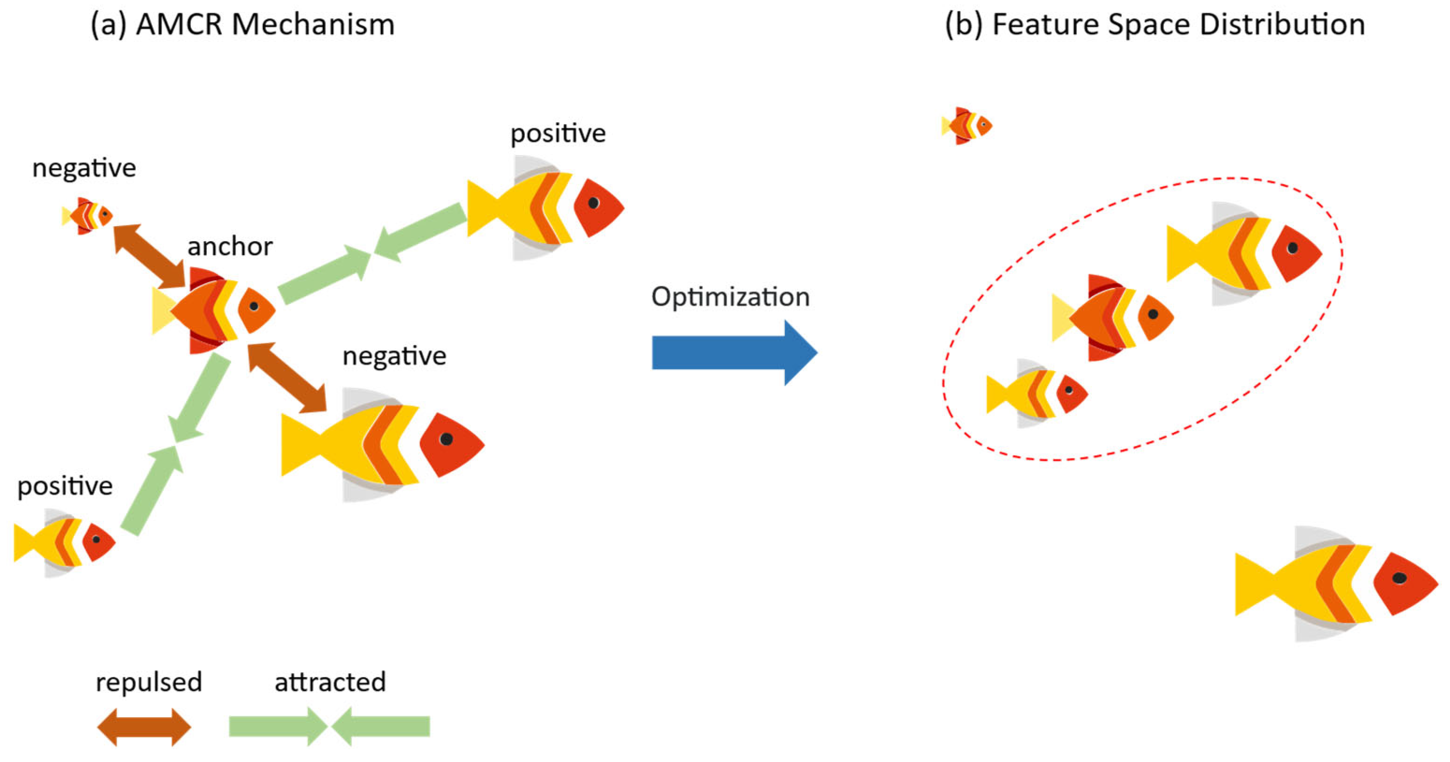
- We designed and introduced the adaptive multi-scale contrastive regression (AMCR) loss function, specifically tailored for imbalanced regression, into the task of fish biometric parameter prediction. Combined with the efficient channel attention (ECA) module, this approach significantly improved the model’s predictive accuracy on long-tail data and its overall robustness.
- We proposed and validated a complete technical pipeline, from high-accuracy model training to extreme lightweight deployment. By employing a general structured pruning technique based on dependency graphs (DepGraph), implemented via the Torch-Pruning (v1.5.2) library, we substantially compressed the model’s parameter count and computational load by 44.1% and 41.7%, respectively, while maintaining or even improving prediction accuracy.
- Through extensive comparative experiments and ablation studies, we systematically validated the independent contributions and synergistic effects of each innovative module within our proposed framework. This work provides solid empirical evidence and establishes a new performance benchmark for future model design and optimization strategies in this field. The comprehensive performance of our method on the bass biometric prediction task is illustrated in Figure 1, visually substantiating the above contributions.
2. Materials and Methods
2.1. Dataset Description
2.1.1. Data Acquisition and Scenario Design
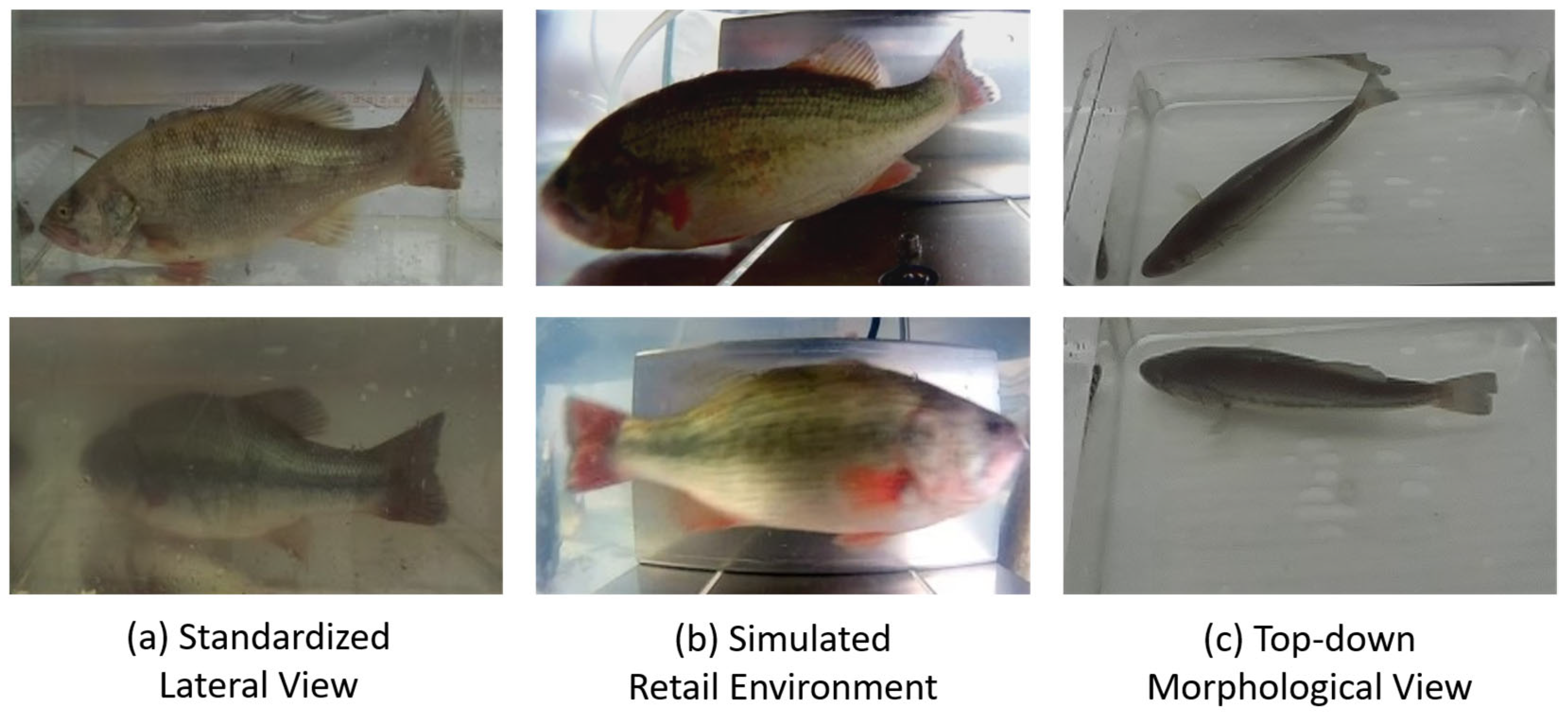
- Standardized lateral view for on-farm monitoring: In this scenario, we placed the fish in a glass tank and captured images laterally from the outside of the tank. This approach was designed to acquire high-quality images with a clean background, uniform lighting, and relatively standard fish poses, serving as ideal conditions for the model to learn baseline morphological data. This scenario was conducted in a controlled environment at the Xiangtan aquaculture base with the objective of acquiring standard lateral-view images rich in information for precise modeling. We captured images of 60 fish using a ZED 2i stereo camera (Stereolabs, San Francisco, CA, USA). To challenge and enhance the model’s environmental adaptability, this scenario specifically included two critical conditions: clear water and simulated turbid water (see Figure 2a). This was intended to train the model to cope with varying levels of water transparency. In this stage, approximately 660 high-quality data entries, each comprising an RGB image and its corresponding depth map, were collected.
- Simulated retail environment for market-chain tracking: In contrast to Scenario 1, this scenario utilized a waterproof high-definition camera to capture footage underwater, inside a tank that simulated a retail environment. This design was intended to replicate more challenging real-world conditions, including light refraction from underwater imaging, dynamic illumination from surface reflections, more complex backgrounds, and the uncooperative, non-rigid poses of fish in a confined space. We procured 30 live specimens from an aquatic market in Changsha and recorded underwater lateral-view videos using a waterproof high-definition camera (Fuli, Model A8, Shenzhen, China). This scenario simulated the temporary holding tanks common at retail terminals. The core challenges were complex dynamic lighting (e.g., surface reflections), diverse backgrounds (retail tanks), and uncooperative, non-rigid poses adopted by the fish due to spatial constraints. Using key-frame extraction techniques, we obtained approximately 340 dynamic images featuring diverse poses (see Figure 2b), which significantly enhanced the dataset’s diversity and robustness for complex real-world scenarios.
- Top-down morphological view for on-farm biomass estimation: At the Jishou aquaculture base, we again utilized the ZED 2i camera to capture images of 30 fish from a direct top-down perspective (see Figure 2c). This viewpoint is crucial for biomass estimation and is intended to complement the information provided by lateral views. The fish width and dorsal contour data available from this perspective are key variables for accurately estimating the condition factor and body weight. This provided the necessary data dimensionality for the model to overcome the limitations of a single viewpoint and establish a more precise non-linear mapping between body length and weight.
2.1.2. Ground Truth Annotation and Quality Control
2.1.3. Dataset Statistical Analysis and Partitioning
2.1.4. Data Preparation and Augmentation
2.2. AMCR: Adaptive Multi-Scale Contrastive Regression Loss Function
2.2.1. Problem Formulation
2.2.2. Imbalanced Contrastive Regression

2.2.3. Theoretical Insight
2.3. Overall Model Architecture
2.3.1. Feature Extraction Backbone
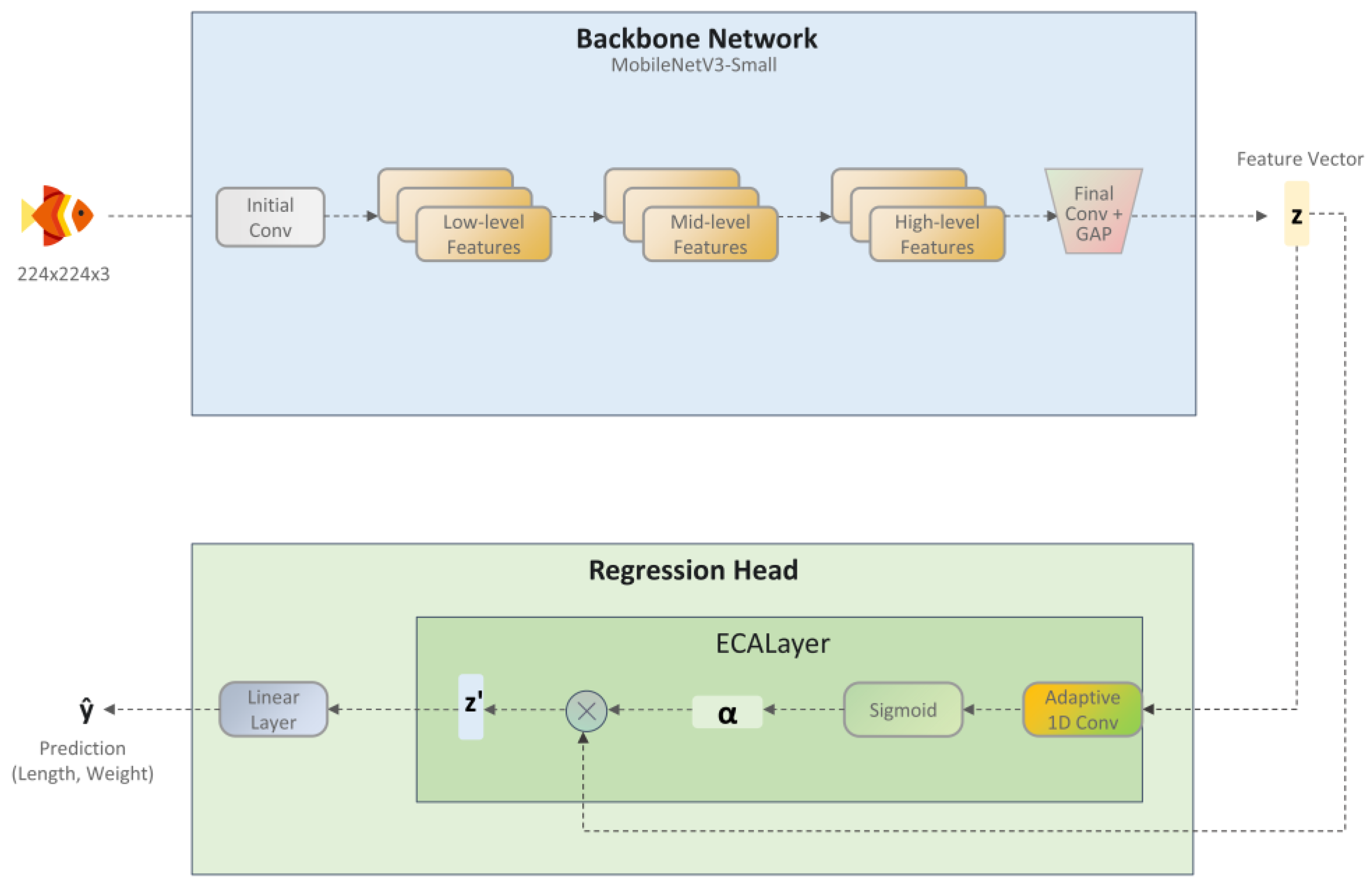
2.3.2. Efficient Channel Attention Regression Head
- Avoidance of dimensionality reduction bottlenecks: The SE module facilitates channel interaction through two FC layers: the first compresses the channel dimension, and the second restores it. However, the authors of ECA-Net demonstrated through experiments that this dimensionality reduction is not essential for learning effective channel attention and may even be detrimental to model performance. Consequently, the ECA module discards the dimensionality reduction step and performs interactions directly on the original channel dimensions, thereby eliminating this potential bottleneck.
- Efficient local cross-channel interaction: ECA proposes an efficient local interaction strategy where the attention weight for each channel is learned by considering information from only its nearest neighboring channels, rather than engaging in global interaction with all channels. This strategy can be implemented with high efficiency using a one-dimensional (1D) convolution with a kernel size of
2.4. Design of the Hybrid Loss Function
2.5. Model Compression and Fine-Tuning
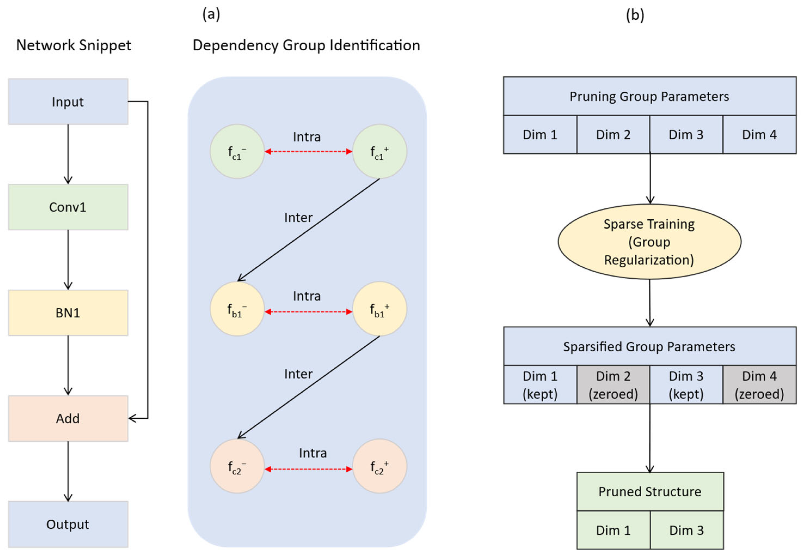
2.5.1. General Structured Pruning Based on Dependency Graphs
2.5.2. Pruning and Fine-Tuning Pipeline
- Dependency-graph construction and group identification: The well-trained, high-accuracy bass prediction model, along with a sample input, was fed into the torch-pruning framework. The framework automatically performed network decomposition, constructed the dependency graph D, and identified all indivisible dependency groups through graph traversal.
- Group-level sparsity training: The model underwent a short period of retraining on the original training set, with group-level sparsity regularization applied. This step learned a consistent sparsity mask for each dimension within every dependency group, thereby identifying redundant dimensions.
- Pruning execution: guided by the sparsity masks learned during training, all dimensions or entire dependency groups identified as redundant were iteratively removed until a predefined global pruning ratio was achieved. Key safeguard: to preserve the core prediction functionality, the final linear layer of the regression head was explicitly excluded from the pruning scope.
- Fine-tuning: Structured pruning inevitably causes a temporary degradation in model performance. After the pruning was completed, the compacted model was fine-tuned on the original training set. This fine-tuning process involved training for a limited number of epochs with a small learning rate. The objective was to help the model recover and optimize its predictive accuracy on the new, pruned architecture, ultimately aiming to match or even surpass its pre-pruning performance level.
3. Results
3.1. Experimental Setup and Evaluation Metrics
3.1.1. Experimental Environment and Hyperparameter Settings
3.1.2. Evaluation Metrics
- Root mean square error (RMSE): . This metric measures the degree of dispersion between predicted and true values and is more sensitive to larger errors. A lower RMSE value indicates higher prediction accuracy.
- Mean absolute error (MAE): . This metric reflects the average absolute magnitude of the prediction error and is less sensitive to outliers. It provides a direct representation of the actual level of prediction error.
- Mean absolute percentage error (MAPE): . This metric quantifies the relative error in percentage form, eliminating the influence of scale and facilitating comparisons across prediction tasks with different dimensions.
- Coefficient of determination (R2): . This metric indicates the explanatory power of the model for the variance in the target variable. Its value ranges from 0 to 1, with a value closer to 1 signifying a better model fit.
3.2. Comparative Experiments
3.2.1. Performance Analysis of Length and Weight Prediction
3.2.2. Comprehensive Evaluation
3.3. Analysis of Model Compression and Fine-Tuning Results
3.3.1. Inherent Efficiency of ECR-MobileNet
3.3.2. Extreme Lightweighting Achieved Through Structured Pruning
3.3.3. Comprehensive Evaluation of Performance and Efficiency
3.4. Ablation Studies
3.4.1. Ablation Analysis on the Length Prediction Task
3.4.2. Ablation Analysis on the Weight Prediction Task
3.5. Visualization Analysis
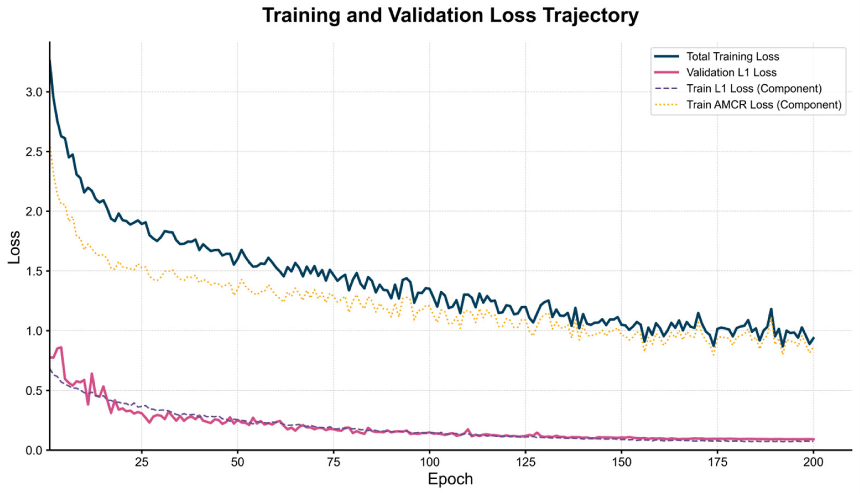
3.5.1. Analysis of the Training Process
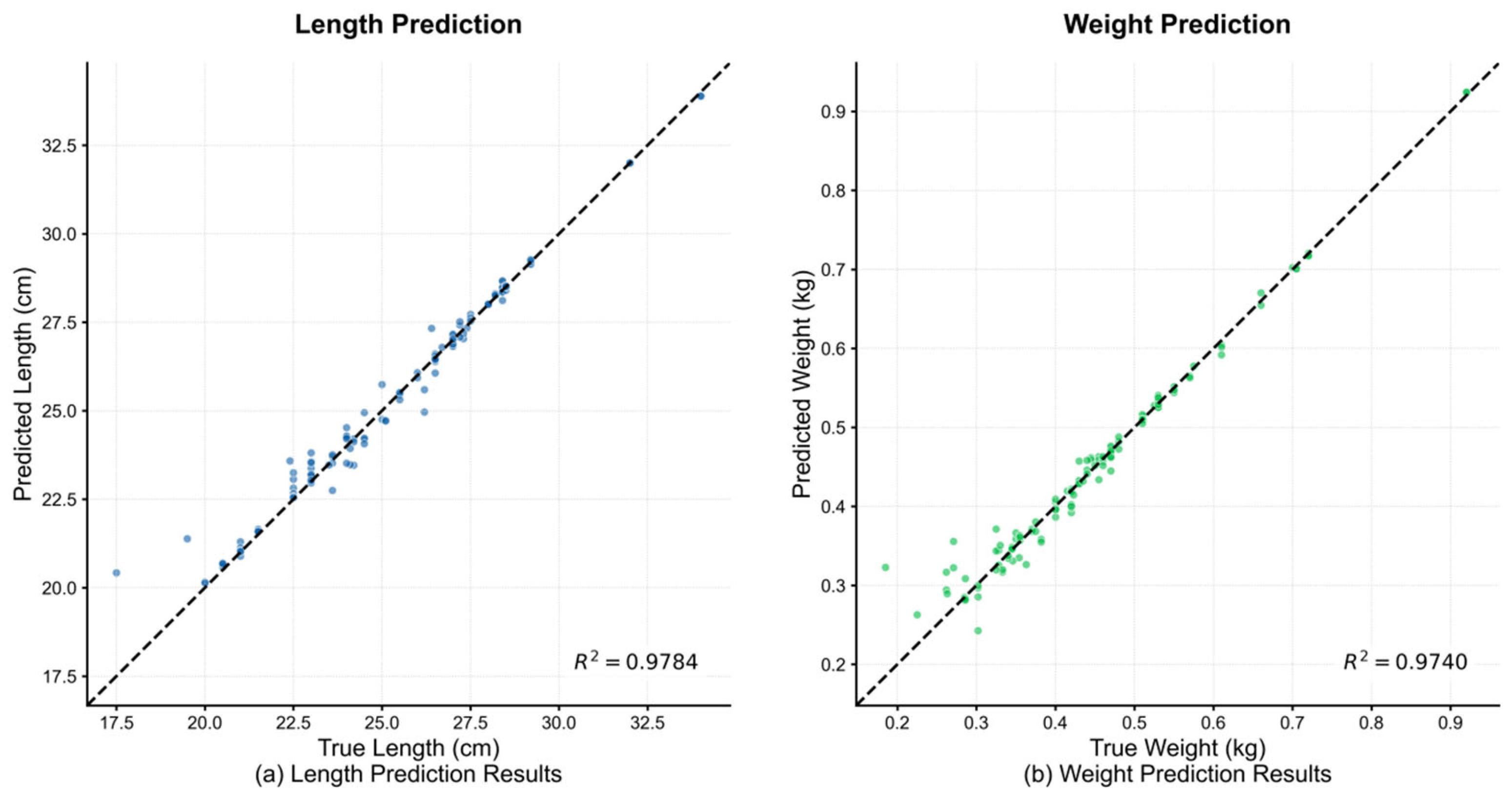
3.5.2. Visualization of Prediction Performance
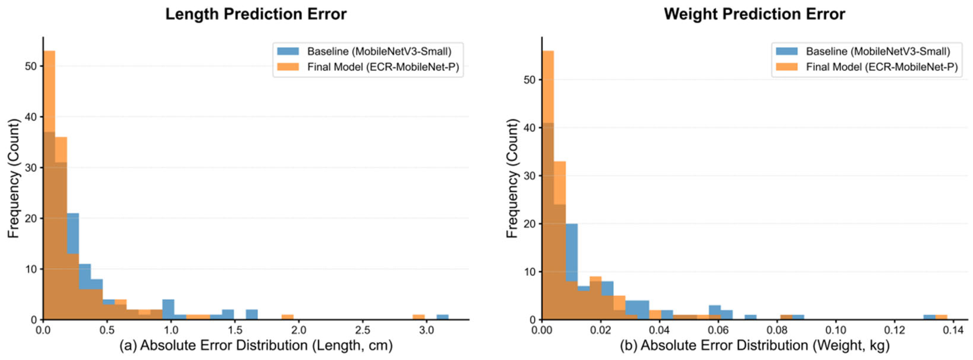
3.5.3. Comparative Analysis of Error Distributions
4. Discussion
4.1. Interpretation of Results
- ECA mechanism: By adaptively adjusting channel weights, the ECA module [36] enhanced the model’s ability to focus on critical features, which is crucial for distinguishing salient morphological landmarks from a cluttered and dynamic underwater background.
- AMCR loss function: Through its contrastive learning strategy, AMCR dynamically constructed positive and negative pair relationships among samples, effectively mitigating the data imbalance problem and ensuring fair predictions across different fish sizes.
- Structured pruning: By employing the dependency-graph-based DepGraph pruning technique [37], the parameter count of ECR-MobileNet-P was reduced from 0.93 M to 0.52 M, and the computational load from 0.12 GFLOPs to 0.07 GFLOPs—a reduction in 44.1% and 41.7%, respectively. This method is particularly suitable for compact architectures like MobileNetV3, as it correctly identifies and preserves complex inter-layer dependencies, preventing structural damage that simpler pruning methods might cause. After fine-tuning, the model’s performance not only recovered but surpassed that of the original model, validating the potential of pruning as an optimization tool.
4.2. Comparison with Existing Literature
4.3. Implications for Aquaculture
4.4. Limitations
- The current dataset was primarily collected from specific aquaculture environments in Hunan Province, which may not fully represent the diverse farming conditions (e.g., water quality, illumination) found in different regions globally. Therefore, the model’s generalization ability in other environments requires further validation.
- Although this study enhanced the model’s robustness through a multi-scene dataset, extreme conditions—such as severely turbid water or rapidly swimming fish—may still affect prediction accuracy. This necessitates further testing under such challenging scenarios.
- The pruned model exhibited a marginal decrease in certain metrics compared to its unpruned counterpart. While its overall performance remained superior to the baseline models, this trade-off between efficiency and performance must be carefully considered in practical applications.
4.5. Future Research Directions
- Validating the model’s performance on different fish species and across diverse geographical regions to assess its generalization capabilities [5].
- Exploring techniques such as quantization, neural architecture search (NAS), or hybrid CNN-Transformer architectures to further reduce the model’s computational demands while maintaining or even enhancing prediction accuracy [35].
4.6. Theoretical and Methodological Contributions
- AMCR provides a novel solution to the data imbalance problem in regression tasks by dynamically constructing positive and negative pair relationships among samples. Its methodology is potentially generalizable to other domains where imbalanced regression is a challenge [35].
- This research demonstrates that pruning can serve as a form of regularization by reducing redundant parameters, not merely as a tool for reducing model complexity. This finding challenges the conventional notion that pruning inevitably sacrifices accuracy, thereby offering new insights for model compression research.
5. Conclusions
Author Contributions
Funding
Institutional Review Board Statement
Informed Consent Statement
Data Availability Statement
Conflicts of Interest
References
- Agriculture Organization of the United Nations. The State of World Fisheries and Aquaculture; Food and Agriculture Organization of the United Nations: Rome, Italy, 2018. [Google Scholar]
- Bureau of Fisheries, Ministry of Agriculture and Rural Affairs of the People’s Republic of China. China Fishery Statistical Yearbook 2024; China Agriculture Press: Beijing, China, 2024. [Google Scholar]
- Liu, Y.; Lei, M.; Victor, H.; Wang, Z.; Yu, C.; Zhang, G.; Wang, Y. The optimal feeding frequency for largemouth bass (Micropterus salmoides) reared in pond and in-pond-raceway. Aquaculture 2022, 548, 737464. [Google Scholar] [CrossRef]
- Barreto, M.O.; Rey Planellas, S.; Yang, Y.; Phillips, C.; Descovich, K. Emerging indicators of fish welfare in aquaculture. Rev. Aquac. 2022, 14, 343–361. [Google Scholar] [CrossRef]
- Aung, T.; Abdul Razak, R.; Rahiman Bin Md Nor, A. Artificial intelligence methods used in various aquaculture applications: A systematic literature review. J. World Aquac. Soc. 2025, 56, e13107. [Google Scholar] [CrossRef]
- Li, D.; Hao, Y.; Duan, Y. Nonintrusive methods for biomass estimation in aquaculture with emphasis on fish: A review. Rev. Aquac. 2020, 12, 1390–1411. [Google Scholar] [CrossRef]
- Barton, B.A. Stress in fishes: A diversity of responses with particular reference to changes in circulating corticosteroids. Integr. Comp. Biol. 2002, 42, 517–525. [Google Scholar] [CrossRef]
- Wang, Q.; Ye, W.; Tao, Y.; Li, Y.; Lu, S.; Xu, P.; Qiang, J. Transport stress induces oxidative stress and immune response in juvenile largemouth bass (Micropterus salmoides): Analysis of oxidative and immunological parameters and the gut microbiome. Antioxidants 2023, 12, 157. [Google Scholar] [CrossRef]
- Fruciano, C. Measurement error in geometric morphometrics. Dev. Genes Evol. 2016, 226, 139–158. [Google Scholar] [CrossRef]
- Tresor, K.K.A.; Mathieu, D.Y.; Leonard, T.; Sebastino, D.C.K. Length-Weight Relationships and Condition Factor of 33 Freshwater Fish Species in the Recently Impounded Soubré Reservoir in Côte d’Ivoire (West Africa). J. Fish. Environ. 2023, 47, 106–118. [Google Scholar]
- Saberioon, M.; Gholizadeh, A.; Cisar, P.; Pautsina, A.; Urban, J. Application of machine vision systems in aquaculture with emphasis on fish: State-of-the-art and key issues. Rev. Aquac. 2017, 9, 369–387. [Google Scholar] [CrossRef]
- Zion, B. The use of computer vision technologies in aquaculture—A review. Comput. Electron. Agric. 2012, 88, 125–132. [Google Scholar] [CrossRef]
- Krizhevsky, A.; Sutskever, I.; Hinton, G.E. ImageNet classification with deep convolutional neural networks. Commun. ACM 2017, 60, 84–90. [Google Scholar] [CrossRef]
- Krizhevsky, A.; Sutskever, I.; Hinton, G.E. Imagenet classification with deep convolutional neural networks. In Proceedings of the Advances in Neural Information Processing Systems 25 (NIPS 2012), Lake Tahoe, NV, USA, 3–6 December 2012. [Google Scholar]
- He, K.; Zhang, X.; Ren, S.; Sun, J. Deep residual learning for image recognition. In Proceedings of the IEEE Conference on Computer Vision and Pattern Recognition, Las Vegas, NV, USA, 27–30 June 2016; pp. 770–778. [Google Scholar]
- Kamilaris, A.; Prenafeta-Boldú, F.X. Deep learning in agriculture: A survey. Comput. Electron. Agric. 2018, 147, 70–90. [Google Scholar] [CrossRef]
- Dosovitskiy, A.; Beyer, L.; Kolesnikov, A.; Weissenborn, D.; Zhai, X.; Unterthiner, T.; Dehghani, M.; Minderer, M.; Heigold, G.; Gelly, S.; et al. An image is worth 16x16 words: Transformers for image recognition at scale. arXiv 2020, arXiv:2010.11929. [Google Scholar]
- Khan, S.; Naseer, M.; Hayat, M.; Zamir, S.W.; Khan, F.S.; Shah, M. Transformers in vision: A survey. ACM Comput. Surv. (CSUR) 2022, 54, 1–41. [Google Scholar] [CrossRef]
- Cheng, Y.; Wang, D.; Zhou, P.; Zhang, T. A survey of model compression and acceleration for deep neural networks. arXiv 2017, arXiv:1710.09282. [Google Scholar]
- Howard, A.G.; Zhu, M.; Chen, B.; Kalenichenko, D.; Wang, W.; Weyand, T.; Andreetto, M.; Adam, H. Mobilenets: Efficient convolutional neural networks for mobile vision applications. arXiv 2017, arXiv:1704.04861. [Google Scholar] [CrossRef]
- Sandler, M.; Howard, A.; Zhu, M.; Zhmoginov, A.; Chen, L.C. Mobilenetv2: Inverted residuals and linear bottlenecks. In Proceedings of the IEEE Conference on Computer Vision and Pattern Recognition, Salt Lake City, UT, USA, 18–22 June 2018; pp. 4510–4520. [Google Scholar]
- Howard, A.; Sandler, M.; Chu, G.; Chen, L.C.; Chen, B.; Tan, M.; Wang, W.; Zhu, Y.; Pang, R.; Vasudevan, V.; et al. Searching for mobilenetv3. In Proceedings of the IEEE/CVF International Conference on Computer Vision, Seoul, Republic of Korea, 27 October–2 November 2019; pp. 1314–1324. [Google Scholar]
- Zhang, X.; Zhou, X.; Lin, M.; Sun, J. Shufflenet: An extremely efficient convolutional neural network for mobile devices. In Proceedings of the IEEE Conference on Computer Vision and Pattern Recognition, Salt Lake City, UT, USA, 18–22 June 2018; pp. 6848–6856. [Google Scholar]
- Ma, N.; Zhang, X.; Zheng, H.T.; Sun, J. Shufflenet v2: Practical guidelines for efficient cnn architecture design. In Proceedings of the European Conference on Computer Vision (ECCV), Munich, Germany, 8–14 September 2018; pp. 116–131. [Google Scholar]
- Han, K.; Wang, Y.; Tian, Q.; Guo, J.; Xu, C.; Xu, C. Ghostnet: More features from cheap operations. In Proceedings of the IEEE/CVF Conference on Computer Vision and Pattern Recognition, Seattle, WA, USA, 13–19 June 2020; pp. 1580–1589. [Google Scholar]
- Tang, Y.; Han, K.; Guo, J.; Xu, C.; Xu, C.; Wang, Y. GhostNetv2: Enhance cheap operation with long-range attention. Adv. Neural Inf. Process. Systems 2022, 35, 9969–9982. [Google Scholar]
- Liu, Z.; Hao, Z.; Han, K.; Tang, Y.; Wang, Y. Ghostnetv3: Exploring the training strategies for compact models. arXiv 2024, arXiv:2404.11202. [Google Scholar]
- Zhang, T.; Yang, Y.; Liu, Y.; Liu, C.; Zhao, R.; Li, D.; Shi, C. Fully automatic system for fish biomass estimation based on deep neural network. Ecol. Inform. 2024, 79, 102399. [Google Scholar] [CrossRef]
- Rani, S.J.; Ioannou, I.; Swetha, R.; Lakshmi, R.D.; Vassiliou, V. A novel automated approach for fish biomass estimation in turbid environments through deep learning, object detection, and regression. Ecol. Inform. 2024, 81, 102663. [Google Scholar] [CrossRef]
- Yan, Z.; Hao, L.; Yang, J.; Zhou, J. Real-time underwater fish detection and recognition based on CBAM-YOLO network with lightweight design. J. Mar. Sci. Eng. 2024, 12, 1302. [Google Scholar] [CrossRef]
- Zheng, T.; Wu, J.; Kong, H.; Zhao, H.; Qu, B.; Liu, L.; Yu, H.; Zhou, C. A video object segmentation-based fish individual recognition method for underwater complex environments. Ecol. Inform. 2024, 82, 102689. [Google Scholar] [CrossRef]
- Xue, Y.; Palstra, A.P.; Blonk, R.; Mussgnug, R.; Khan, H.A.; Komen, H.; Bastiaansen, J.W. Genetic analysis of swimming performance in rainbow trout (Oncorhynchus mykiss) using image traits derived from deep learning. Aquaculture 2025, 606, 742607. [Google Scholar] [CrossRef]
- Oord, A.; Li, Y.; Vinyals, O. Representation learning with contrastive predictive coding. arXiv 2018, arXiv:1807.03748. [Google Scholar]
- Keramati, M.; Meng, L.; Evans, R.D. Conr: Contrastive regularizer for deep imbalanced regression. arXiv 2023, arXiv:2309.06651. [Google Scholar]
- Yang, Y.; Zha, K.; Chen, Y.; Wang, H.; Katabi, D. Delving into deep imbalanced regression. In Proceedings of the International Conference on Machine Learning PMLR, Virtual Event, 18–24 July 2021; pp. 11842–11851. [Google Scholar]
- Wang, Q.; Wu, B.; Zhu, P.; Li, P.; Zuo, W.; Hu, Q. ECA-Net: Efficient channel attention for deep convolutional neural networks. In Proceedings of the IEEE/CVF Conference on Computer Vision and Pattern Recognition, Seattle, WA, USA, 13–19 June 2020; pp. 11534–11542. [Google Scholar]
- Fang, G.; Ma, X.; Song, M.; Mi, M.B.; Wang, X. Depgraph: Towards any structural pruning. In Proceedings of the IEEE/CVF Conference on Computer Vision and Pattern Recognition, Vancouver, BC, Canada, 17–24 June 2023; pp. 16091–16101. [Google Scholar]
- Saleh, A.; Sheaves, M.; Rahimi Azghadi, M. Computer vision and deep learning for fish classification in underwater habitats: A survey. Fish Fish. 2022, 23, 977–999. [Google Scholar] [CrossRef]
- Zhao, Y.; Qin, H.; Xu, L.; Yu, H.; Chen, Y. A review of deep learning-based stereo vision techniques for phenotype feature and behavioral analysis of fish in aquaculture. Artif. Intell. Rev. 2025, 58, 7. [Google Scholar] [CrossRef]
- Goodfellow, I.; Pouget-Abadie, J.; Mirza, M.; Xu, B.; Warde-Farley, D.; Ozair, S.; Courville, A.; Bengio, Y. Generative adversarial networks. Commun. ACM 2020, 63, 139–144. [Google Scholar] [CrossRef]
- He, K.; Fan, H.; Wu, Y.; Xie, S.; Girshick, R. Momentum contrast for unsupervised visual representation learning. In Proceedings of the IEEE/CVF Conference on Computer Vision and Pattern Recognition, Seattle, WA, USA, 13–19 June 2020; pp. 9729–9738. [Google Scholar]

| Dataset | No. of Images | Total Length Range (cm) | Weight Range (g) | Mean Total Length ± SD (cm) | Mean Weight ± SD (g) |
|---|---|---|---|---|---|
| Training Set | 1026 | 17.5–34.0 | 158–920 | 24.6 ± 2.6 | 419 ± 121 |
| Validation Set | 127 | 17.5–34.0 | 158–920 | 24.9 ± 3.1 | 427 ± 129 |
| Test Set | 131 | 17.5–34.0 | 158–920 | 24.4 ± 2.9 | 411 ± 118 |
| Total | 1284 | 17.5–34.0 | 158–920 | 24.6 ± 2.6 | 419 ± 121 |
| Data Subset | Resize | Horizontal Flip (p) | Random Rotation | Color Jitter (Brightness, Contrast, Saturation, Hue) | Random Grayscale (p) | Normalized |
|---|---|---|---|---|---|---|
| Training Set View 1 | 224 × 224 | 0.5 | ±20° | (0.3, 0.3, 0.3, 0.1) | 0.1 | √ |
| Training Set View 2 | 224 × 224 | 0.5 | ±15° | (0.2, 0.2, 0.2, 0.0) | × | √ |
| Validation/Test Set | 224 × 224 | × | × | × | × | √ |
| Parameter Type | Value |
|---|---|
| Optimizer | AdamW |
| Initial Learning Rate | 1 × 10⁻³ |
| Batch Size | 16 |
| Training Epochs | 200 |
| Learning Rate Scheduler | Cosine Annealing |
| Loss Function | Mean Squared Error (MSE) |
| Models | RMSE | MAE | MAPE | R2 |
|---|---|---|---|---|
| Edgevit_xxs | 0.6024 | 0.3245 | 1.39% | 0.9576 |
| Efficientformerv2_s2 | 0.4933 | 0.3162 | 1.32% | 0.9716 |
| Efficientnetv2 | 0.4979 | 0.2604 | 1.12% | 0.9710 |
| Ghostv3 | 0.5189 | 0.2935 | 1.25% | 0.9685 |
| Mobilenetv2 | 0.6178 | 0.3190 | 1.38% | 0.9554 |
| Mobilenetv3_large | 0.4328 | 0.2571 | 1.07% | 0.9781 |
| Mobilenetv3_small | 0.5234 | 0.3105 | 1.32% | 0.9680 |
| Mobilevit_s | 0.6243 | 0.4255 | 1.75% | 0.9545 |
| Repvit | 0.5502 | 0.3254 | 1.32% | 0.9646 |
| Resnet50 | 0.5465 | 0.2711 | 1.16% | 0.9651 |
| Shufflenetv2_x1.0 | 0.4457 | 0.2911 | 1.22% | 0.9768 |
| Tiny_vit | 0.6109 | 0.3801 | 1.58% | 0.9564 |
| Vit_small | 1.0401 | 0.7650 | 3.10% | 0.8736 |
| Fastvit_sa12 | 0.6380 | 0.4002 | 1.66% | 0.9524 |
| ECR-Mobilenet (ours) | 0.4565 | 0.2149 | 0.93% | 0.9757 |
| ECR-Mobilenet-P (ours) | 0.4296 | 0.2310 | 0.99% | 0.9784 |
| Models | RMSE | MAE | MAPE | R2 |
|---|---|---|---|---|
| Edgevit_xxs | 0.0274 | 0.0163 | 4.92% | 0.9525 |
| Efficientformerv2_s2 | 0.0239 | 0.0154 | 4.43% | 0.9637 |
| Efficientnetv2 | 0.0287 | 0.0139 | 4.44% | 0.9479 |
| Ghostv3 | 0.0228 | 0.0133 | 4.00% | 0.9672 |
| Mobilenetv2 | 0.0244 | 0.0134 | 3.80% | 0.9621 |
| Mobilenetv3_large | 0.0234 | 0.0134 | 3.92% | 0.9654 |
| Mobilenetv3_small | 0.0253 | 0.0153 | 4.61% | 0.9595 |
| Mobilevit_s | 0.0269 | 0.0184 | 4.92% | 0.9540 |
| Repvit | 0.0265 | 0.0158 | 4.46% | 0.9554 |
| Resnet50 | 0.0275 | 0.0134 | 4.20% | 0.9522 |
| Shufflenetv2_x1.0 | 0.0224 | 0.0140 | 4.05% | 0.9680 |
| Tiny_vit | 0.0237 | 0.0156 | 4.47% | 0.9643 |
| Vit_small | 0.0446 | 0.0308 | 7.86% | 0.8741 |
| Fastvit_sa12 | 0.0287 | 0.0187 | 5.33% | 0.9479 |
| ECR-Mobilenet (ours) | 0.0228 | 0.0109 | 3.50% | 0.9671 |
| ECR-Mobilenet-P (ours) | 0.0202 | 0.0108 | 3.31% | 0.9740 |
| Models | Parameters (M) | GFLOPs | CPU Latency (ms) | Memory (MB) |
|---|---|---|---|---|
| Edgevit_xxs | 3.77 | 1.10 | 31.13 | 14.42 |
| Efficientformer_s2 | 12.13 | 2.48 | 73.19 | 46.97 |
| Efficientnetv2 | 20.18 | 5.44 | 74.45 | 77.56 |
| Ghostv3 | 6.85 | 0.87 | 112.19 | 26.58 |
| Mobilenetv2 | 2.22 | 0.61 | 29.29 | 8.62 |
| Mobilenetv3_large | 4.20 | 0.44 | 22.89 | 16.13 |
| Mobilenetv3_small | 1.51 | 0.11 | 12.30 | 5.84 |
| Mobilevit_s | 4.93 | 2.48 | 63.72 | 18.88 |
| Repvit_0.9 | 6.40 | 2.27 | 53.29 | 24.65 |
| Resnet50 | 23.51 | 8.26 | 66.14 | 89.89 |
| Mhufflenetv2_x1.0 | 1.25 | 0.30 | 20.87 | 4.85 |
| Tiny_vit | 5.07 | 2.37 | 45.01 | 21.21 |
| Vit_small | 21.66 | 6.44 | 43.27 | 82.65 |
| Fastvit_sa12 | 10.55 | 3.00 | 58.50 | 40.41 |
| ECR-Mobilenet (ours) | 0.93 | 0.12 | 14.46 | 3.59 |
| ECR-Mobilenet-P (ours) | 0.52 | 0.07 | 10.19 | 2.00 |
| L1 Loss | ECA + Linear | AMCR | RMSE | MAE | MAPE | R2 |
|---|---|---|---|---|---|---|
| × | × | × | 0.5234 | 0.3105 | 1.32% | 0.9680 |
| √ | × | × | 0.5814 | 0.2771 | 1.21% | 0.9605 |
| × | √ | × | 0.5135 | 0.2969 | 1.26% | 0.9692 |
| × | × | √ | 0.5265 | 0.2952 | 1.25% | 0.9676 |
| √ | √ | × | 0.4951 | 0.2397 | 1.04% | 0.9714 |
| √ | × | √ | 0.5414 | 0.2552 | 1.10% | 0.9658 |
| × | √ | √ | 0.5050 | 0.2651 | 1.13% | 0.9702 |
| √ | √ | √ | 0.4565 | 0.2149 | 0.93% | 0.9757 |
| L1 Loss | ECA + Linear | AMCR | RMSE | MAE | MAPE | R2 |
|---|---|---|---|---|---|---|
| × | × | × | 0.0253 | 0.0153 | 4.61% | 0.9595 |
| √ | × | × | 0.0248 | 0.0123 | 3.88% | 0.9609 |
| × | √ | × | 0.0240 | 0.0141 | 4.22% | 0.9634 |
| × | × | √ | 0.0251 | 0.0145 | 4.36% | 0.9600 |
| √ | √ | × | 0.0233 | 0.0116 | 3.55% | 0.9665 |
| √ | × | √ | 0.0265 | 0.0119 | 3.85% | 0.9554 |
| × | √ | √ | 0.0232 | 0.0134 | 4.04% | 0.9657 |
| √ | √ | √ | 0.0228 | 0.0109 | 3.50% | 0.9671 |
Disclaimer/Publisher’s Note: The statements, opinions and data contained in all publications are solely those of the individual author(s) and contributor(s) and not of MDPI and/or the editor(s). MDPI and/or the editor(s) disclaim responsibility for any injury to people or property resulting from any ideas, methods, instructions or products referred to in the content. |
© 2025 by the authors. Licensee MDPI, Basel, Switzerland. This article is an open access article distributed under the terms and conditions of the Creative Commons Attribution (CC BY) license (https://creativecommons.org/licenses/by/4.0/).
Share and Cite
Peng, H.; Ouyang, C.; Yang, L.; Deng, J.; Tan, M.; Luo, Y.; Hu, W.; Jiang, P.; Wang, Y. ECR-MobileNet: An Imbalanced Largemouth Bass Parameter Prediction Model with Adaptive Contrastive Regression and Dependency-Graph Pruning. Animals 2025, 15, 2443. https://doi.org/10.3390/ani15162443
Peng H, Ouyang C, Yang L, Deng J, Tan M, Luo Y, Hu W, Jiang P, Wang Y. ECR-MobileNet: An Imbalanced Largemouth Bass Parameter Prediction Model with Adaptive Contrastive Regression and Dependency-Graph Pruning. Animals. 2025; 15(16):2443. https://doi.org/10.3390/ani15162443
Chicago/Turabian StylePeng, Hao, Cheng Ouyang, Lin Yang, Jingtao Deng, Mingyu Tan, Yahui Luo, Wenwu Hu, Pin Jiang, and Yi Wang. 2025. "ECR-MobileNet: An Imbalanced Largemouth Bass Parameter Prediction Model with Adaptive Contrastive Regression and Dependency-Graph Pruning" Animals 15, no. 16: 2443. https://doi.org/10.3390/ani15162443
APA StylePeng, H., Ouyang, C., Yang, L., Deng, J., Tan, M., Luo, Y., Hu, W., Jiang, P., & Wang, Y. (2025). ECR-MobileNet: An Imbalanced Largemouth Bass Parameter Prediction Model with Adaptive Contrastive Regression and Dependency-Graph Pruning. Animals, 15(16), 2443. https://doi.org/10.3390/ani15162443


