Author Contributions
Conceptualization, A.O.B., D.W.B. and K.D.M.; methodology, A.O.B. and D.W.B.; software, D.W.B. and L.L.T.; validation, A.O.B., L.L.T. and P.P.; formal analysis, A.O.B., D.W.B., S.U. and L.L.T.; investigation, A.O.B. and P.P.; resources, D.W.B.; data curation, A.O.B.; writing—original draft preparation, A.O.B.; writing—review and editing, A.O.B., D.W.B., K.D.M., P.P. and S.U.; visualization, A.O.B. and D.W.B.; supervision, D.W.B. and S.U.; project administration, D.W.B.; funding acquisition, D.W.B. All authors have read and agreed to the published version of the manuscript.
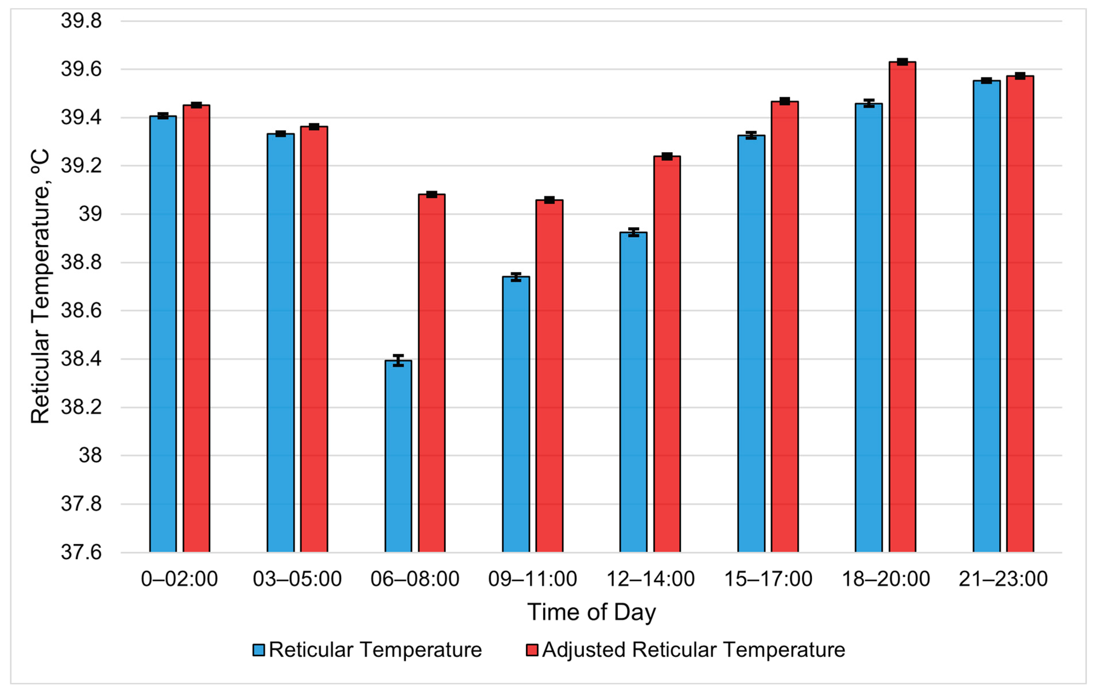
Figure 1.
Least-square means of reticular temperature (RT) and adjusted reticular temperature (ART) averaged for each 3 h period during the summer study period. All RT periods are different (p < 0.01), except periods 03:00 to 05:00 and 15:00 to 17:00 (p = 0.71). Similarly, all ART periods are different (p < 0.01), except periods 00:00 to 02:00 and 15:00 to 17:00 (p = 0.1). Error bars represent standard errors.
Figure 2.
Relationship between the adjusted reticular temperature and wet bulb globe temperature (WBGT) over the course of a day using 3 h data. Columns are the least-square means of the adjusted reticular temperature, and error bars represent standard errors. Values are averages of the entire summer study period.
Figure 3.
A visual representation of the cubic relationship between the adjusted reticular temperature and wet bulb globe temperature using 3 h data. This line was calculated from the coefficients obtained from the repeated-measures analysis (
Table 7). The values on the
x-axis were chosen to better illustrate the shape of the relationship and may exceed those observed in the study.
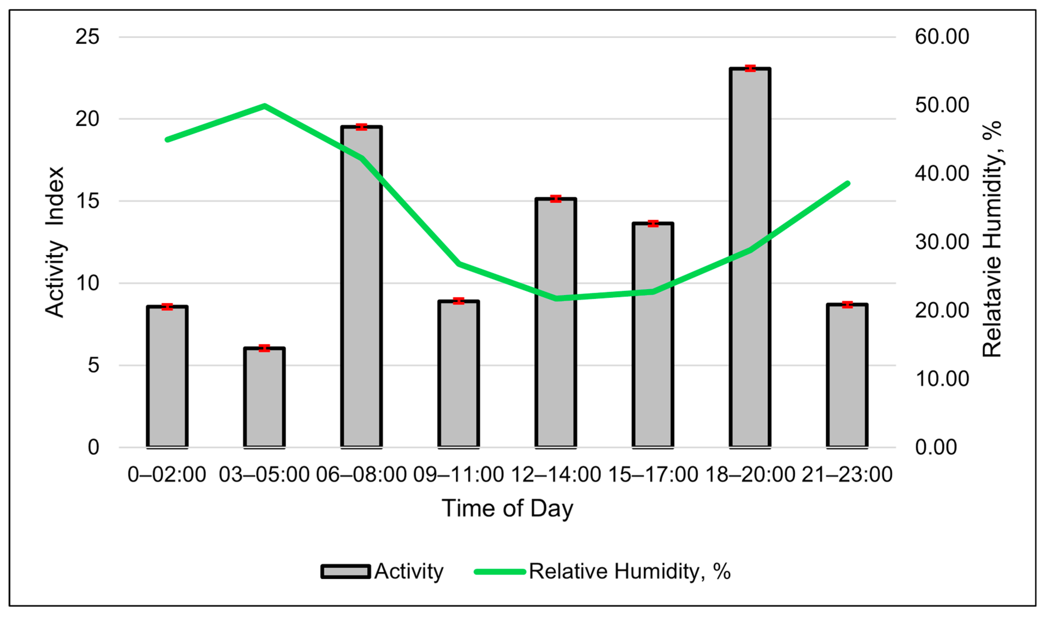
Figure 4.
Relationship between the SmaXtec activity index and relative humidity throughout the day during using 3 h data. Columns are the least-square means of the activity index, and the error bars represent standard errors. Values are averages of the entire summer study period.
Figure 4.
Relationship between the SmaXtec activity index and relative humidity throughout the day during using 3 h data. Columns are the least-square means of the activity index, and the error bars represent standard errors. Values are averages of the entire summer study period.
Figure 5.
A visual representation of the cubic relationship between the activity index and relative humidity using 3 h data. This line was calculated from the coefficients obtained from the repeated-measures analysis (
Table 7). The values on the
x-axis are given to better illustrate the shape of the relationship and may exceed those observed in the study.
Figure 6.
Relationship between the SmaXtec rumination index and wind speed (m/s) over the course of a day, using 3 h data. Columns are the least-square means of the rumination index, and the error bars represent standard errors. Values are averages of the entire summer study period. No differences in rumination index were detected (p > 0.05) among time periods.
Figure 7.
A visual representation of the cubic relationship between the rumination index and wind speed (m/s) using 3 h data. This line was calculated from the coefficients obtained from the repeated-measures analysis (
Table 7). The values on the
x-axis are given to better illustrate the shape of the relationship and may exceed those observed in the study.
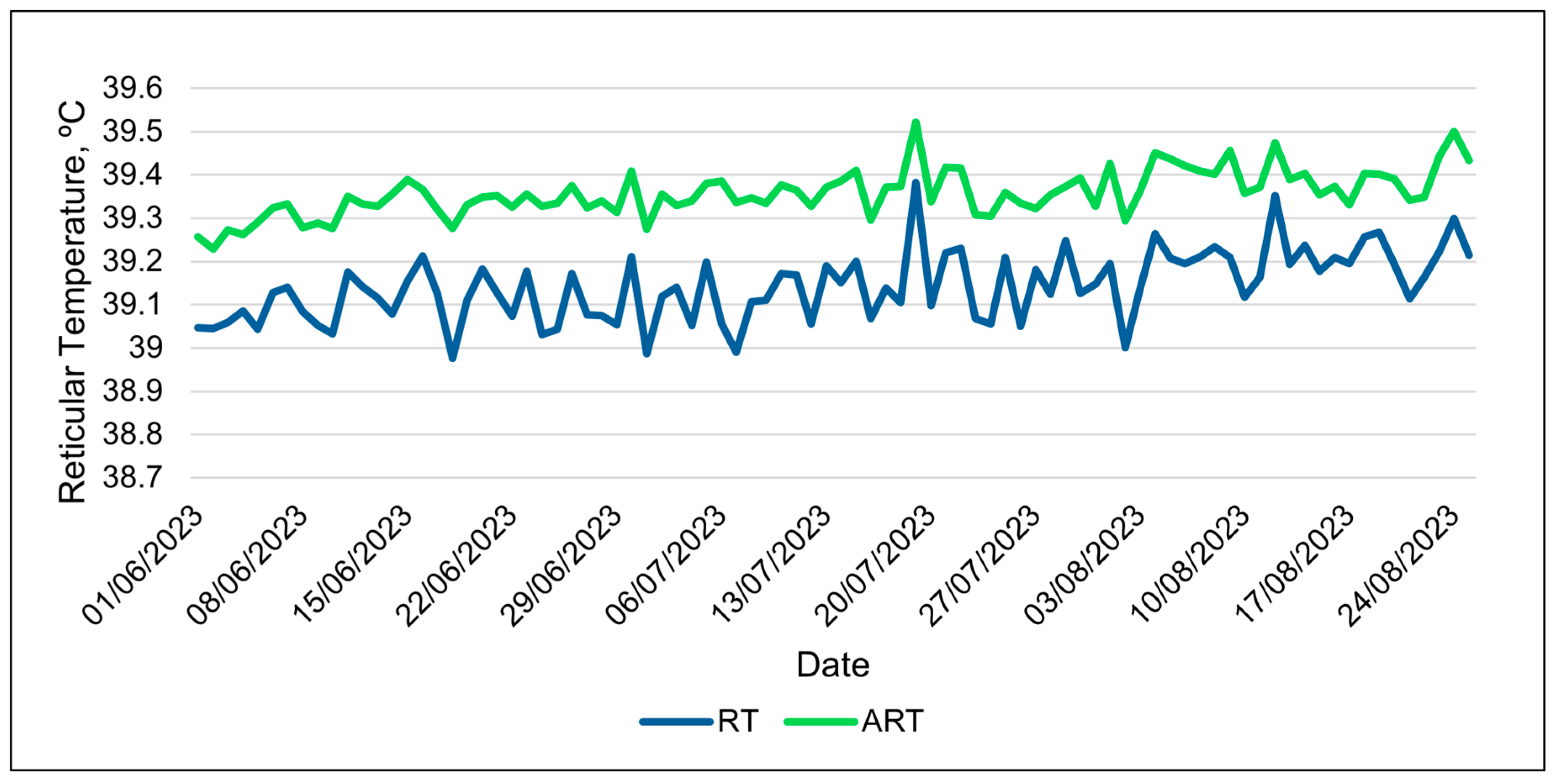
Figure 8.
Daily changes in adjusted reticular temperature (ART) and reticular temperature (RT) during the entire summer study using 24 h data.
Figure 8.
Daily changes in adjusted reticular temperature (ART) and reticular temperature (RT) during the entire summer study using 24 h data.
Figure 9.
A visual representation of the quadratic relationship between the adjusted reticular temperature and the wet bulb globe temperature (WBGT), using 24 h data (daily averages). This line was calculated from the coefficients obtained from the repeated-measures analysis. The values on the x-axis are included to better illustrate the shape of the relationship and may exceed those observed in the study.
Figure 10.
A visual representation of the cubic relationship between the activity index and relative humidity, using 24 h data (daily averages). This line was calculated from the coefficients obtained from the repeated-measures analysis. The values on the x-axis are used to better illustrate the shape of the relationship and may exceed those observed in the study.
Figure 11.
A visual representation of the linear relationship between the water intake index and relative humidity, using 24 h data (daily averages). This line was calculated from the coefficients obtained from the repeated-measures analysis. The values on the x-axis are used to better illustrate the shape of the relationship and may exceed those observed in the study.
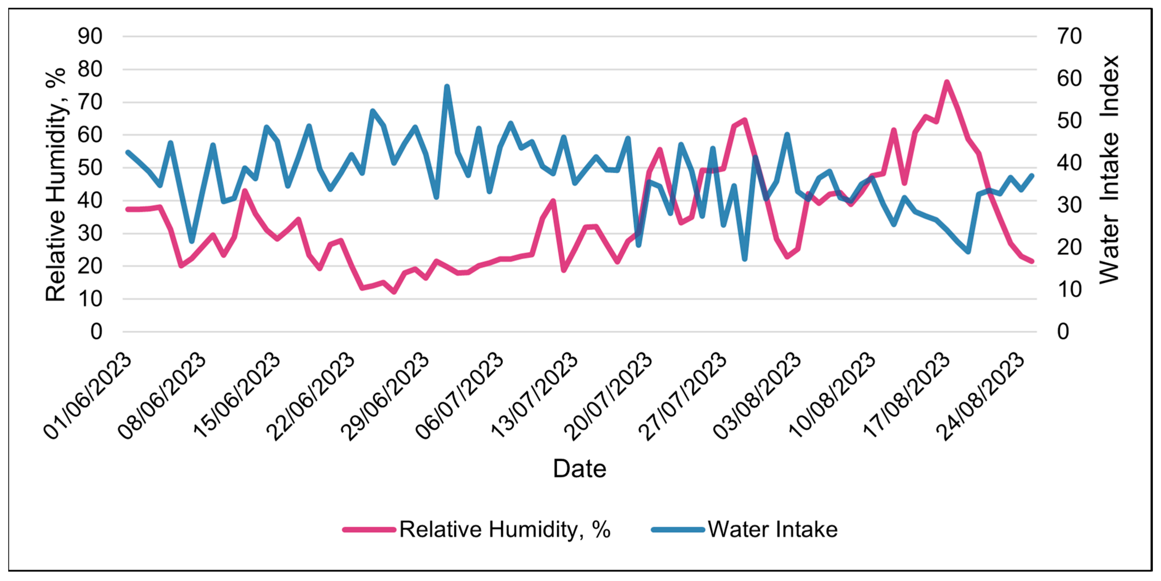
Figure 12.
Daily relationship between SmaXtec’s water intake index and relative humidity during the entire summer study using 24 h data.
Figure 12.
Daily relationship between SmaXtec’s water intake index and relative humidity during the entire summer study using 24 h data.
Figure 13.
Daily relationship between reticular temperature and water intake index during the entire summer study using 24 h data.
Figure 13.
Daily relationship between reticular temperature and water intake index during the entire summer study using 24 h data.
Table 1.
Maximum, minimum and mean weather metric values based on 5 min weather data during the summer study period for the weather metrics used in the statistical analyses.
Table 1.
Maximum, minimum and mean weather metric values based on 5 min weather data during the summer study period for the weather metrics used in the statistical analyses.
| Metric 1 | AT (°C) | RH (%) | Wind Speed (m/s) | THI (°C) | WBGT (°C) | Solar Load (Watts) |
|---|
| Mean | 24.11 | 34.31 | 3.40 | 20.17 | 18.72 | 301.37 |
| Max | 39.40 | 100.00 | 14.40 | 27.17 | 30.83 | 938.00 |
| Min | 7.00 | 1.96 | 0.00 | 8.00 | 1.94 | 0.00 |
Table 2.
Description of time periods used in the 3 h analyses (hours of each period).
Table 2.
Description of time periods used in the 3 h analyses (hours of each period).
| Time Period | Hour |
|---|
| 0 | 00:00–02:59 |
| 1 | 03:00–05:59 |
| 2 | 06:00–08:59 |
| 3 | 09:00–11:59 |
| 4 | 12:00–14:59 |
| 5 | 15:00–17:59 |
| 6 | 18:00–20:59 |
| 7 | 21:00–23:59 |
Table 3.
Coefficients, standard errors, R-squared values, p-values and Akaike Information Criterion (AIC) scores from simple regression between the observed activity and the activity index and regression between the observed rumination and the rumination index.
Table 3.
Coefficients, standard errors, R-squared values, p-values and Akaike Information Criterion (AIC) scores from simple regression between the observed activity and the activity index and regression between the observed rumination and the rumination index.
| | Coefficient | SE | R2 | p-Value | AIC |
|---|
| Activity | 2.821 | 0.172 | 0.27 | <0.0001 | 7507.3 |
| Rumination | 9.343 | 2.150 | 0.03 | <0.0001 | 7466.4 |
Table 4.
Coefficients, standard errors, p-values and Akaike Information Criterion (AIC) scores for each function from the polynomial regression with repeated measures between the observed activity and the activity index with linear, quadratic and cubic relationships.
Table 4.
Coefficients, standard errors, p-values and Akaike Information Criterion (AIC) scores for each function from the polynomial regression with repeated measures between the observed activity and the activity index with linear, quadratic and cubic relationships.
| Polynomial Regression: Activity |
|---|
| Linear | |
| Coefficient X | 2.05 |
| SE | 0.189 |
| p-value | <0.0001 |
| AIC | 7181.5 |
| Quadratic | |
| Coefficient X | 3.524 |
| SE | 0.656 |
| p-value | <0.0001 |
| Coefficient X2 | −0.0481 |
| SE | 0.021 |
| p-value | <0.05 |
| AIC | 7182 |
| Cubic | |
| Coefficient X | 8.366 |
| SE | 1.707 |
| p-value | <0.0001 |
| Coefficient X2 | −0.391 |
| SE | 0.113 |
| p-value | <0.01 |
| Coefficient X3 | 0.007 |
| SE | 0.002 |
| p-value | <0.01 |
| AIC | 7183.5 |
Table 5.
Correlation coefficients among weather metrics used in the statistical analyses. Weather metrics include ambient temperature (AT), relative humidity (RH), wind speed, temperature–humidity index (THI), wet bulb globe temperature (WBGT) and solar load.
Table 5.
Correlation coefficients among weather metrics used in the statistical analyses. Weather metrics include ambient temperature (AT), relative humidity (RH), wind speed, temperature–humidity index (THI), wet bulb globe temperature (WBGT) and solar load.
| | AT | RH | Wind Speed | THI | WBGT | Solar Load |
|---|
| AT | 1 | | | | | |
| RH | −0.515 | 1 | | | | |
| Wind Speed | 0.446 | −0.469 | 1 | | | |
| THI | 0.972 | −0.344 | 0.368 | 1 | | |
| WBGT | 0.848 | −0.163 | 0.198 | 0.897 | 1 | |
| Solar Load | 0.566 | −0.436 | 0.347 | 0.509 | 0.705 | 1 |
Table 6.
Pearson coefficient correlation results between the weather metrics (wet bulb globe temperature (WBGT), relative humidity (RH) and ambient temperature (AT)) provided from Klimo Insight using weather data from the Prescott Regional Airport and a Kestrel 5400AG cattle heat load tracker.
Table 6.
Pearson coefficient correlation results between the weather metrics (wet bulb globe temperature (WBGT), relative humidity (RH) and ambient temperature (AT)) provided from Klimo Insight using weather data from the Prescott Regional Airport and a Kestrel 5400AG cattle heat load tracker.
| Weather Metric | Correlation |
|---|
| AT | 0.93 |
| RH | 0.92 |
| WBGT | 0.87 |
Table 7.
The two best models describing the relationships between each SmaXtec metric (activity index, reticular temperature (RT), adjusted reticular temperature (ART) and rumination index) and the corresponding weather variables (ambient temperature (AT), relative humidity (RH), wind speed, wet bulb globe temperature (WBGT) and solar load) determined by the lowest Akaike Information Criterion (AIC) score using the 3 h data. The model type and corresponding standard errors and p-values are given for each coefficient in each model.
Bolus
Metric | Weather Variable | Model Type | Function(s) | Coefficient | SE | p-Value | Model AIC |
|---|
| Activity | RH | Cubic | Linear | 25.4078 | 3.0790 | <0.0001 | 40,095.2 |
| | | | Quadratic | −41.2614 | 7.4537 | <0.0001 | |
| | | | Cubic | 21.9897 | 5.3174 | <0.0001 | |
| Activity | Solar Load | Linear | Linear | −0.0107 | 0.0007 | <0.0001 | 40,110.3 |
| RT | Solar Load | Linear | Linear | −0.0007 | 0.0001 | <0.0001 | 5941.8 |
| RT | RH | Linear | Linear | 0.2519 | 0.0289 | <0.0001 | 5981.9 |
| ART | WBGT | Cubic | Linear | −0.0938 | 0.0111 | <0.0001 | −3876.6 |
| | | | Quadratic | 0.0053 | 0.0007 | <0.0001 | |
| | | | Cubic | −0.0001 | 0.0000 | <0.0001 | |
| ART | RH | Cubic | Linear | 1.0712 | 0.1730 | <0.0001 | −3851.2 |
| | | | Quadratic | −2.0390 | 0.3985 | <0.0001 | |
| | | | Cubic | 1.1051 | 0.2795 | <0.0001 | |
| Rumination | Wind Speed | Cubic | Linear | 120.1400 | 61.7424 | 0.0517 | 116,545 |
| | | | Quadratic | −33.1055 | 14.8805 | 0.0261 | |
| | | | Cubic | 2.9257 | 1.0748 | 0.0065 | |
| Rumination | AT | Quadratic | Linear | −71.8109 | 23.4900 | 0.0022 | 116,556.2 |
| | | | Quadratic | 1.4327 | 0.4488 | 0.0014 | |
Table 8.
The top two weather metrics, including the relative humidity (RH), solar load, wet bulb globe temperature (WBGT), wind speed and ambient temperature (AT), associated with changes in the SmaXtec indices, which included the activity index, reticular temperature (RT), adjusted reticular temperature (ART), rumination index and water intake index, from both the 3 h and 24 h data sets. The table provides the model rank, model type and Akaike Information Criterion (AIC) score for each model.
| Data Type | SmaXtec Metric | Model Rank | Weather Metric | Model Type | AIC |
|---|
| 3-h | Activity Index | 1 | RH | Cubic | 40,095.2 |
| 3-h | Activity Index | 2 | Solar Load | Linear | 40,110.3 |
| 24-h | Activity Index | 1 | RH | Cubic | 3202.1 |
| 24-h | Activity Index | 2 | Solar Load | Quadratic | 3270 |
| 3-h | RT | 1 | Solar Load | Linear | 5941.8 |
| 3-h | RT | 2 | RH | Linear | 5981.9 |
| 24-h | RT | 1 | RH | Linear | −961.1 |
| 24-h | RT | 2 | WBGT | Linear | −946.6 |
| 3-h | ART | 1 | WBGT | Cubic | −3876.6 |
| 3-h | ART | 2 | RH | Cubic | −3851.2 |
| 24-h | ART | 1 | WBGT | Quadratic | −1499.2 |
| 24-h | ART | 2 | THI | Linear | −1498.4 |
| 3-h | Rumination Index | 1 | Wind | Cubic | 116,545 |
| 3-h | Rumination Index | 2 | AT | Quadratic | 116,556.2 |
| 24-h | Water Intake | 1 | RH | Linear | 6326 |
| 24-h | Water Intake | 2 | Solar Load | Linear | 6392.1 |
Table 9.
The two best models determined by the lowest Akaike Information Criterion (AIC) score in describing the relationships between SmaXtec metrics, including the activity index, reticular temperature (RT), adjusted reticular temperature (ART) and rumination index, and corresponding weather variables, which included the relative humidity (RH), wet bulb globe temperature (WBGT), temperature–humidity index (THI) and solar load, using the 24 h data. Model types, coefficients, standard errors and p-values are given for each coefficient in each model.
| Bolus Metric | Weather Variable | Model Type | Function(s) | Coefficient | SE | p-Value | Model AIC |
|---|
| Activity | RH | Cubic | Linear | 53.8130 | 7.3369 | <0.0001 | 3202.1 |
| | | | Quadratic | −133.8700 | 18.5300 | <0.0001 | |
| | | | Cubic | 107.7900 | 14.4182 | <0.0001 | |
| Activity | Solar Load | Quadratic | Linear | −0.0618 | 0.0086 | <0.0001 | 3270 |
| | | | Quadratic | 0.0001 | 0.0000 | <0.0001 | |
| RT | RH | Linear | Linear | 0.2403 | 0.0484 | <0.0001 | −961.1 |
| RT | WBGT | Linear | Linear | 0.0101 | 0.0025 | <0.0001 | −946.6 |
| ART | WBGT | Quadratic | Linear | −0.0675 | 0.0211 | 0.0014 | −1499.2 |
| | | | Quadratic | 0.0022 | 0.0006 | 0.0002 | |
| ART | THI | Linear | Linear | 0.0073 | 0.0019 | 0.0002 | −1498.4 |
| Water Intake | RH | Linear | Linear | −32.5000 | 2.1697 | <0.0001 | 6326 |
| Water Intake | Solar Load | Linear | Linear | 0.0907 | 0.0075 | <0.0001 | 6392.1 |


 ,
, 


