
Genomic Predictions of Phenotypes and Pseudo-Phenotypes for Viral Nervous Necrosis Resistance, Cortisol Concentration, Antibody Titer and Body Weight in European Sea Bass

 ,
,  ,
,  ,
,
Abstract
Simple Summary
Abstract
1. Introduction
2. Materials and Methods
2.1. Experimental Fish: Production, Rearing and NNV Challenge Test
2.2. Assessment of Phenotypes for Antibody Titer against NNV and Cortisol Concentration
2.3. Genotyping, Parentage Assignment and Pedigree Reconstruction
2.4. Genome-Wide Association Study
2.5. Prediction of Breeding Values
2.6. Genomic Predictions
2.6.1. Bayesian Regression Models
2.6.2. Random Forest Algorithm
2.6.3. Assessment of Model Performance in Prediction and Classification
3. Results
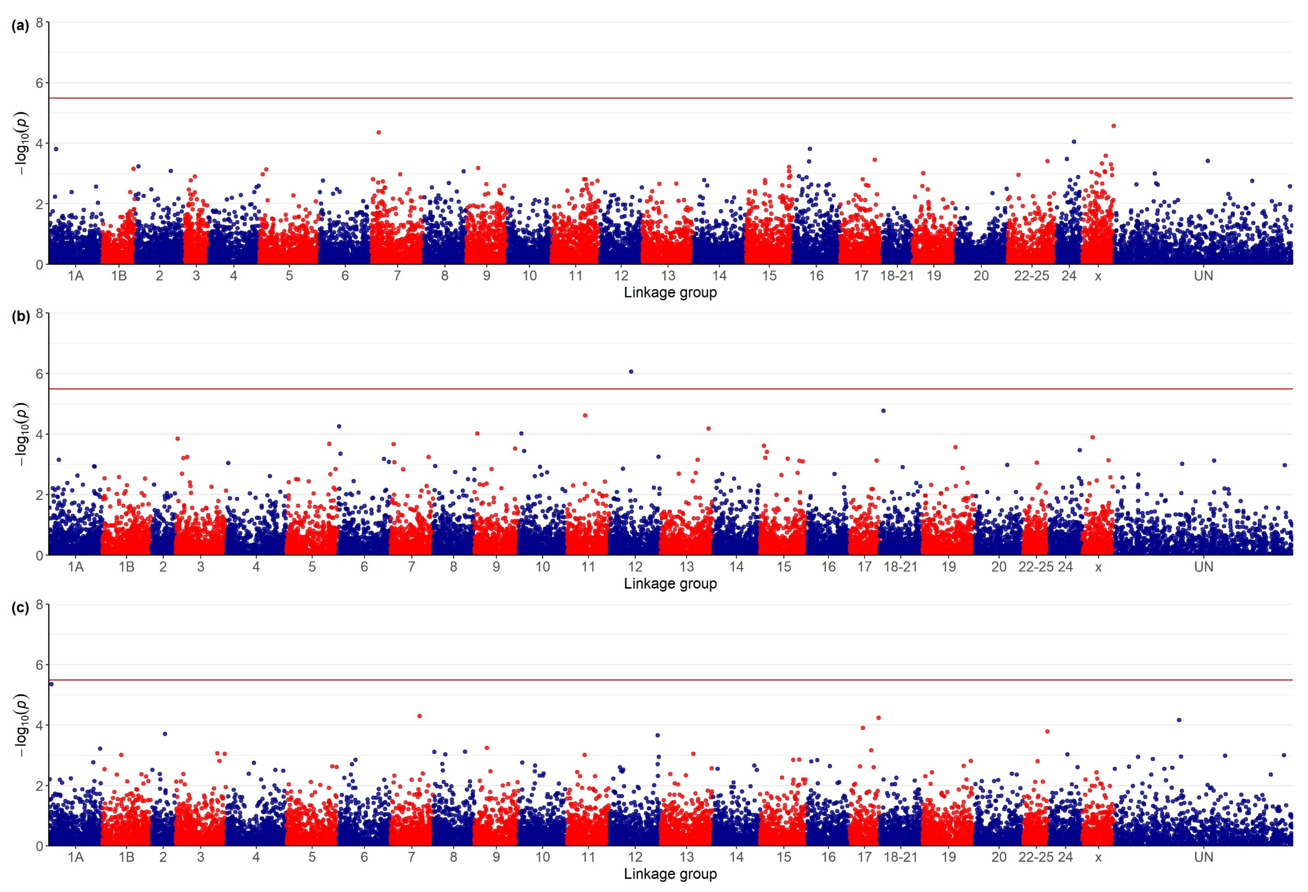
3.1. Genome-Wide Association Study
3.2. Genomic Prediction and Classification
3.2.1. Predictive Ability of Genomic Models
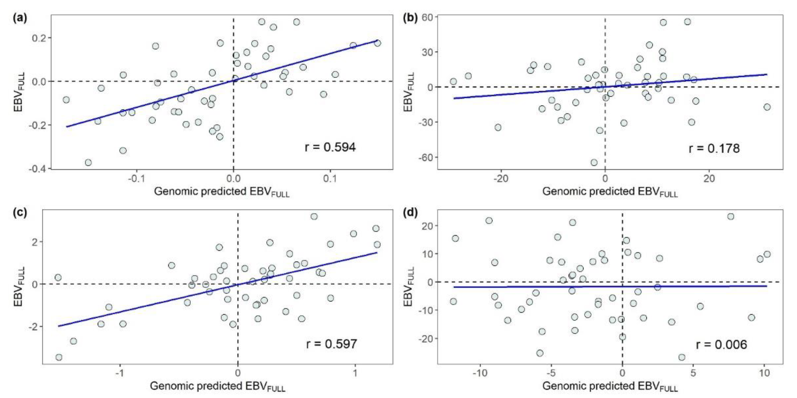
3.2.2. Leave-One-Family-Out Validation
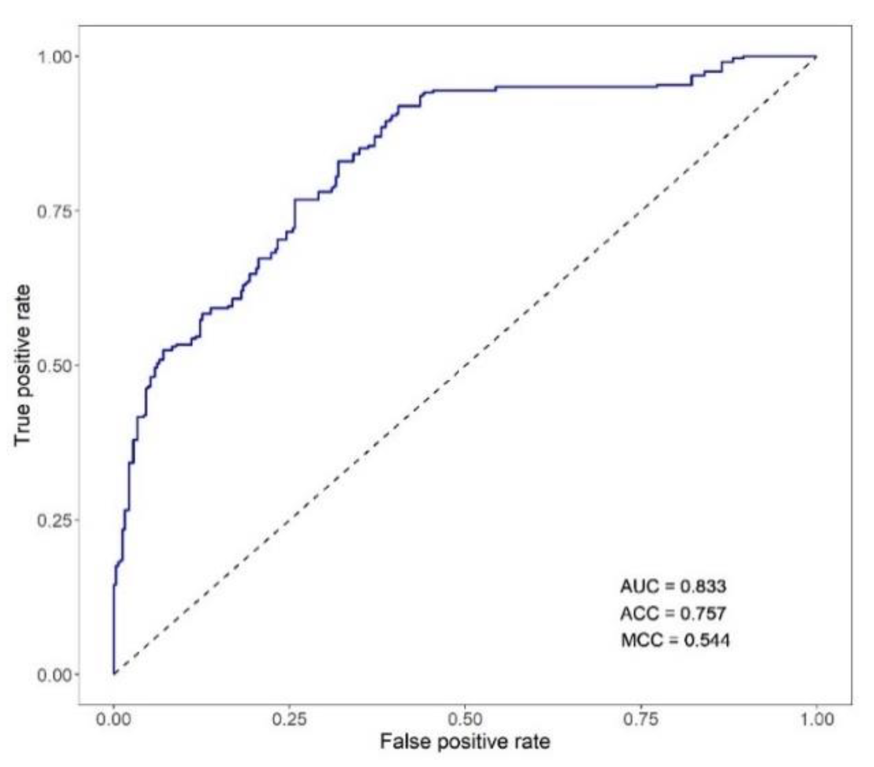
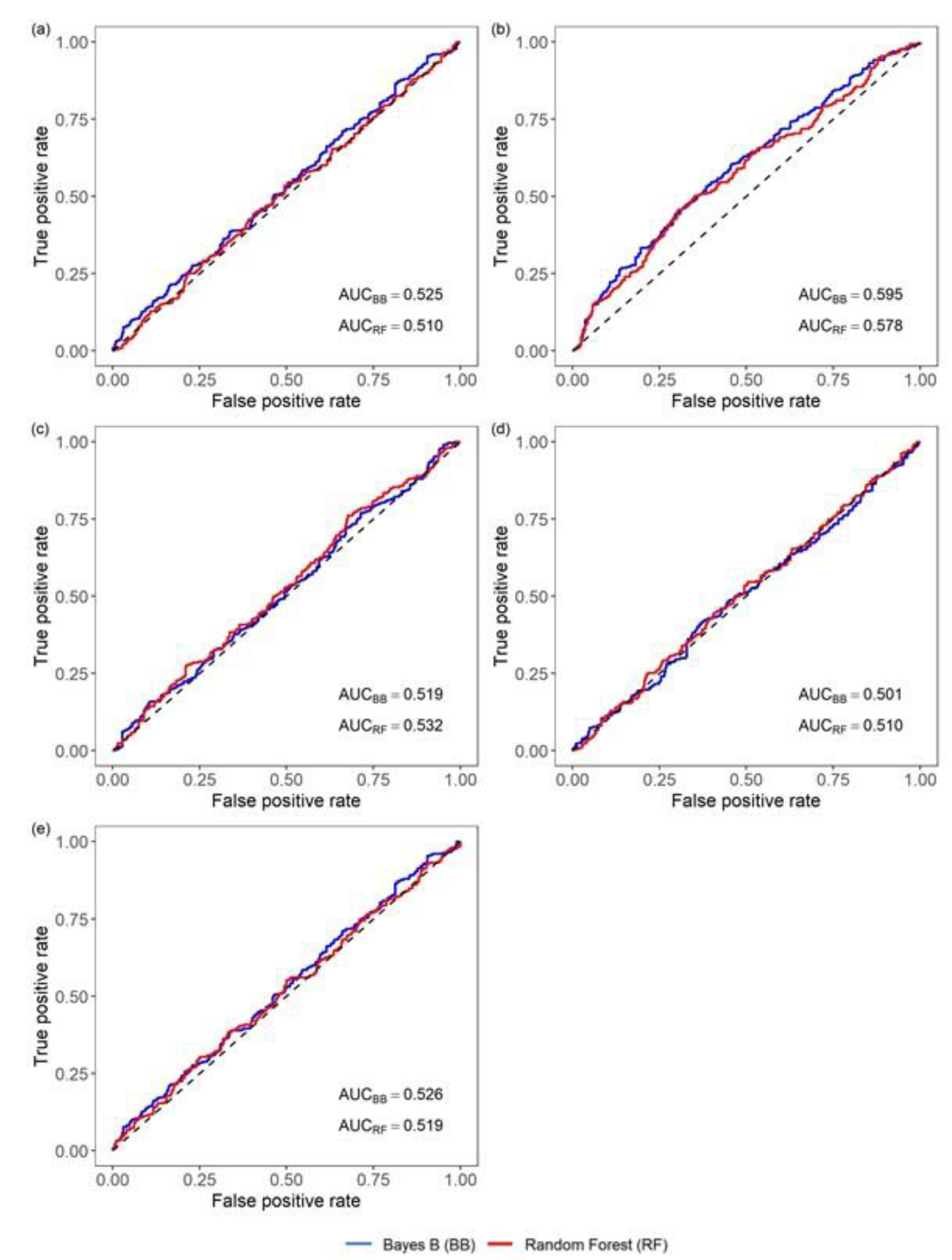
3.2.3. Performance of Classifiers of Viral Nervous Necrosis Mortality
4. Discussion
5. Conclusions
Author Contributions
Funding
Institutional Review Board Statement
Informed Consent Statement
Data Availability Statement
Acknowledgments
Conflicts of Interest
Appendix A


References
- Sonesson, A.K.; Meuwissen, T.H.E. Testing strategies for genomic selection in aquaculture breeding programs. Genet. Sel. Evol. 2009, 41, 37. [Google Scholar] [CrossRef] [PubMed]
- Palaiokostas, C.; Cariou, S.; Bestin, A.; Bruantn, J.S.; Haffray, P.; Morin, T.; Cabon, J.; Allal, F.; Vandeputte, M.; Houston, R.D. Genome-wide association and genomic prediction of resistance to viral nervous necrosis in European sea bass (Dicentrarchus labrax) using RAD sequencing. Genet. Sel. Evol. 2018, 50, 30. [Google Scholar] [CrossRef] [PubMed]
- Palaiokostas, C.; Ferraresso, S.; Franch, R.; Houston, R.; Bargelloni, L. Genomic prediction of resistance to pasteurellosis in gilthead sea bream (Sparus aurata) using 2b-RAD sequencing. G3-Genes Genom. Genet. 2016, 6, 3693–3700. [Google Scholar] [CrossRef] [PubMed]
- Palaiokostas, C.; Kocour, M.; Prchal, M.; Houston, R.D. Accuracy of genomic evaluations of juvenile growth rate in common carp (Cyprinus carpio) using genotyping by sequencing. Front. Genet. 2018, 9, 82. [Google Scholar] [CrossRef]
- Tsai, H.; Hamilton, A.; Tinch, A.E.; Guy, D.R.; Bron, J.E.; Taggart, J.B.; Gharbi, K.; Stear, M.; Matika, O.; Pong-Wong, R.; et al. Genomic prediction of host resistance to sea lice in farmed Atlantic salmon populations. Genet. Sel. Evol. 2016, 48, 47. [Google Scholar] [CrossRef]
- Vallejo, R.; Leeds, T.; Gao, G.; Parsons, J.; Martin, K.; Evenhuis, J.; Fragomeni, B.O.; Wiens, G.D.; Palti, Y. Genomic selection models double the accuracy of predicted breeding values for bacterial cold water disease resistance compared to a traditional pedigree-based model in rainbow trout aquaculture. Genet. Sel. Evol. 2017, 49, 17. [Google Scholar] [CrossRef]
- Bangera, R.; Correa, K.; Lhorente, J.P.; Figueroa, R.; Yáñez, J.M. Genomic predictions can accelerate selection for resistance against Piscirickettsia salmonis in Atlantic salmon (Salmo salar). BMC Genom. 2017, 18, 121. [Google Scholar] [CrossRef]
- Martsikalis, P.V.; Gkafas, G.A.; Palaiokostas, C.; Exadactylos, A. Genomics era on breeding aquaculture stocks. In Organic Aquaculture: Impacts and Future Developments, 1st ed.; Lembo, G., Mente, E., Eds.; Springer Nature: Cham, Switzerland, 2019; pp. 65–77. [Google Scholar]
- Chavanne, H.; Janssen, K.; Hofherr, J.; Contini, F.; Haffray, P.; Komen, H.; Nielsen, E.E.; Bargelloni, L. A comprehensive survey on selective breeding programs and seed market in the European aquaculture fish industry. Aquacult. Int. 2016, 24, 1287–1307. [Google Scholar] [CrossRef]
- Janssen, K.; Chavanne, H.; Berentsen, P.; Komen, H. Impact of selective breeding on European aquaculture. Aquaculture 2016, 472, 8–16. [Google Scholar] [CrossRef]
- Ødegård, J.; Baranski, M.; Gjerde, B.; Gjedrem, T. Methodology for genetic evaluation of disease resistance in aquaculture species, challenges and future prospects. Aquacult. Res. 2011, 42, 103–114. [Google Scholar] [CrossRef]
- Munday, B.L.; Kwang, J.; Moody, N. Betanodavirus infections of teleost fish, a review. J. Fish Dis. 2002, 27, 127–142. [Google Scholar] [CrossRef]
- Faggion, S.; Bertotto, D.; Babbucci, M.; Dalla Rovere, G.; Franch, R.; Bovolenta, M.; Laureau, M.; Pascoli, F.; Toffan, A.; Bargelloni, L.; et al. Resistance to viral nervous necrosis in European sea bass (Dicentrarchus labrax L.), heritability and relationships with body weight; cortisol concentration and antibody titer. Genet. Sel. Evol. 2021, 53, 32. [Google Scholar] [CrossRef] [PubMed]
- Griot, R.; Allal, F.; Phocas, F.; Brard-Fudulea, S.; Morvezen, R.; Bestin, A.; Haffray, P.; François, Y.; Morin, T.; Poncet, C.; et al. Genome-wide association studies for resistance to viral nervous necrosis in three populations of European sea bass (Dicentrarchus labrax) using a novel 57k SNP array DlabChip. Aquaculture 2021, 530, 735930. [Google Scholar] [CrossRef]
- Doan, Q.K.; Vandeputte, M.; Chatain, B.; Haffray, P.; Vergnet, A.; Breuil, G.; Allal, F. Genetic variation of resistance to Viral Nervous Necrosis and genetic correlations with production traits in wild populations of the European sea bass (Dicentrarchus labrax). Aquaculture 2017, 478, 1–8. [Google Scholar] [CrossRef]
- Castanheira, M.F.; Conceição, L.; Millot, S.; Rey, S.; Bégout, M.-L.; Damsgård, B.; Kristiansen, T.; Höglund, E.; Øverli, Ø.; Martins, C.I.M. Coping styles in farmed fish, consequences for aquaculture. Rev. Aquacult. 2015, 9, 23–41. [Google Scholar] [CrossRef]
- MacKenzie, S.; Ribas, L.; Pilarczyk, M.; Capdevila, D.M.; Kadri, S.; Huntingford, F.A. Screening for coping style increases the power of gene expression studies. PLoS ONE 2009, 4, e5314. [Google Scholar] [CrossRef]
- Pottinger, T.G. The stress response in fish-mechanisms, effects and measurement. In Fish Welfare; Branson, E.J., Ed.; Blackwell Publishing Ltd.: Oxford, UK, 2008; pp. 32–44. [Google Scholar]
- Volckaert, F.A.M.; Hellemans, B.; Batargias, C.; Louro, B.; Massault, C.; Van Houdt, J.K.J.; Haley, C.; de Koning, D.-J.; Canario, A.V.M. Heritability of cortisol response to confinement stress in European sea bass Dicentrarchus labrax. Genet. Sel. Evol. 2012, 44, 15. [Google Scholar] [CrossRef]
- Vandeputte, M.; Porte, J.D.; Auperin, B.; Dupont-Nivet, M.; Vergnet, A.; Valotaire, C.; Claireaux, G.; Prunet, P.; Chatain, B. Quantitative genetic variation for post-stress cortisol and swimming performance in growth-selected and control populations of European sea bass (Dicentrarchus labrax). Aquaculture 2016, 455, 1–7. [Google Scholar] [CrossRef]
- Ødegård, J.; Meuwissen, T.H.E. Identity-by-descent genomic selection using selective and sparse genotyping. Genet. Sel. Evol. 2014, 46, 3. [Google Scholar] [CrossRef][Green Version]
- Meuwissen, T.H.E.; Hayes, B.J.; Goddard, M.E. Genomic selection: A paradigm shift in animal breeding. Anim. Front. 2016, 6, 6. [Google Scholar] [CrossRef]
- Robledo, D.; Palaiokostas, C.; Bargelloni, L.; Martínez, P.; Houston, R. Applications of genotyping by sequencing in aquaculture breeding and genetics. Rev. Aquac. 2017, 10, 670–682. [Google Scholar] [CrossRef] [PubMed]
- Meuwissen, T.H.E.; Hayes, B.J.; Goddard, M.E. Prediction of total genetic value using genome-wide dense marker maps. Genetics 2001, 157, 1819–1829. [Google Scholar] [CrossRef] [PubMed]
- Scapigliati, G.; Buonocore, F.; Randelli, E.; Casani, D.; Meloni, S.; Zarletti, G.; Tiberi, M.; Pietretti, D.; Boschi, I.; Manchado, M.; et al. Cellular and molecular immune responses of the sea bass (Dicentrarchus labrax) experimentally infected with betanodavirus. Fish Shellfish Immunol. 2010, 28, 303–311. [Google Scholar] [CrossRef] [PubMed]
- Nuñez-Ortiz, N.; Stocchi, V.; Toffan, A.; Pascoli, F.; Sood, N.; Buonocore, F.; Picchietti, S.; Papeschi, C.; Taddei, A.R.; Thompson, K.D.; et al. Quantitative immunoenzymatic detection of viral encephalopathy and retinopathy virus (betanodavirus) in sea bass Dicentrarchus labrax. J. Fish Dis. 2016, 39, 821–831. [Google Scholar] [CrossRef]
- Bertotto, D.; Poltronieri, C.; Negrato, E.; Majolini, D.; Radaelli, G.; Simontacchi, C. Alternative matrices for cortisol measurement in fish. Aquacult. Res. 2010, 41, 1261–1267. [Google Scholar] [CrossRef]
- Simontacchi, C.; Bongioni, G.; Ferasin, L.; Bono, G. Messa a Punto di un Metodo RIA su Micropiastra per il Dosaggio Diretto del Progestrerone Ematico; Atti XLIX Convegno Nazionale S.I.S.Vet.: Salsomaggiore Terme, PR, Italy, 1995; pp. 343–344. [Google Scholar]
- Wang, S.; Meyer, E.; McKay, J.K.; Matz, M.V. 2b-RAD, a simple and flexible method for genome-wide genotyping. Nat. Methods 2012, 9, 808–810. [Google Scholar] [CrossRef] [PubMed]
- Catchen, J.; Hohenlohe, P.A.; Bassham, S.; Amores, A.; Cresko, W.A. Stacks, an analysis tool set for population genomics. Mol. Ecol. 2013, 22, 3124–3140. [Google Scholar] [CrossRef]
- Tine, M.; Kuhl, H.; Gagnaire, P.-A.; Louro, B.; Desmarais, E.; Martins, R.S.T.; Hecht, J.; Knaust, F.; Belkhir, K.; Klages, S.; et al. The European sea bass genome and its variation provide insight into adaptation to euryhalinity and marine speciation. Nat. Commun. 2014, 5, 5770. [Google Scholar] [CrossRef]
- Sargolzaei, M.; Chesnais, J.P.; Shenkel, F.S. A new approach for efficient genotype imputation using information from relatives. BMC Genom. 2014, 15, 478–489. [Google Scholar] [CrossRef]
- Marshall, T.C.; Slate, J.; Kruuk, L.E.B.; Pemberton, J.M. Statistical confidence for likelihood-based paternity inference in natural populations. Mol. Ecol. 1998, 7, 639–655. [Google Scholar] [CrossRef]
- Kalinowski, S.T.; Taper, M.L.; Marshall, T.C. Revising how the computer program CERVUS accommodates genotyping error increases success in paternity assignment. Mol. Ecol. 2007, 16, 1099–1106. [Google Scholar] [CrossRef] [PubMed]
- Huisman, J. Pedigree reconstruction from SNP data, parentage assignment; sibship clustering and beyond. Mol. Ecol. Res. 2017, 17, 1009–1024. [Google Scholar] [CrossRef] [PubMed]
- Perdry, H.; Dandine-Roulland, C.; Bandyopadhyay, D.; Kettner, L. Package ‘Gaston’: Genetic Data Handling (QC, GRM, LD, PCA) and Linear Mixed Models. Version 1.5.3. Available online: ftp://cran.r-project.org/pub/R/web/packages/gaston/gaston.pdf (accessed on 3 August 2020).
- Wang, L.; Liu, P.; Huang, S.; Ye, B.; Chua, E.; Wan, Z.Y.; Yue, G.H. Genome-wide association study identifies loci associated with resistance to viral nervous necrosis disease in Asian Seabass. Mar. Biotechnol. 2017, 19, 255–265. [Google Scholar] [CrossRef] [PubMed]
- Turner, S.D. qqman: An R package for visualizing GWAS results using Q-Q and manhattan plots. J. Open Source Softw. 2018, 3, 731. [Google Scholar] [CrossRef]
- Legarra, A.; Varona, L.; López de Maturana, E. TM Threshold Model. 2008. Available online: http://snp.toulouse.inra.fr/~alegarra/ (accessed on 15 June 2019).
- Falconer, D.S.; Mackay, T.F.C. Introduction to Quantitative Genetics, 4th ed.; Longman: Harlow, UK, 1996. [Google Scholar]
- Pérez, P.; de Los Campos, G. Genome-wide regression and prediction with the BGLR statistical package. Genetics 2014, 198, 483–495. [Google Scholar] [CrossRef] [PubMed]
- Habier, D.; Fernando, R.; Kizilkaya, K.; Garrick, D. Extension of the Bayesian alphabet for genomic selection. BMC Bioinform. 2011, 12, 186. [Google Scholar] [CrossRef] [PubMed]
- Breiman, L. Random forests. Mach Learn 2001, 45, 5–32. [Google Scholar] [CrossRef]
- Liaw, A.; Wiener, M. Classification and regression by random forest. R News 2002, 2, 18–22. [Google Scholar]
- Ishwaran, H.; Kogalur, U.B. Random Forests for Survival, Regression, and Classification (RF-SRC), R Package Version 2.7.0. 2018. Available online: https://cran.r-project.org/web/packages/randomForestSRC/randomForestSRC.pdf. (accessed on 25 October 2020).
- Fawcett, T. An introduction to ROC analysis. Pattern Recognit. Lett. 2006, 27, 861–874. [Google Scholar] [CrossRef]
- Matthews, B. Comparison of the predicted and observed secondary structure of T4 phage lysozyme. Biochim. Biophys. Acta 1975, 405, 442–451. [Google Scholar] [CrossRef]
- Sing, T.; Sander, O.; Beerenwinkel, N.; Lengauer, T. ROCR, visualizing classifier performance in R. Bioinformatics 2005, 21, 7881. [Google Scholar] [CrossRef] [PubMed]
- Wang, H.; Misztal, I.; Aguilar, I.; Legarra, A.; Muir, W.M. Genome-wide association mapping including phenotypes from relatives without genotypes. Genet. Res. 2012, 94, 73–83. [Google Scholar] [CrossRef] [PubMed]
- Liu, S.; Vallejo, R.L.; Gao, G.; Palti, Y.; Weber, G.M.; Hernandez, A.; Rexroad, C.E., III. Identification of single-nucleotide polymorphism markers associated with cortisol response to crowding in rainbow trout. Mar. Biotechnol. 2015, 17, 328–337. [Google Scholar] [CrossRef] [PubMed]
- Tsai, H.; Hamilton, A.; Tinch, A.E.; Guy, D.R.; Gharbi, K.; Stear, M.; Matika, O.; Bishop, S.C.; Houston, R.D. Genome wide association and genomic prediction for growth traits in juvenile farmed Atlantic salmon using a high density SNP array. BMC Genom. 2015, 16, 969. [Google Scholar] [CrossRef] [PubMed]
- Garcia, A.L.S.; Bosworth, B.; Waldbieser, G.; Misztal, I.; Tsuruta, S.; Lourenco, D.A.L. Development of genomic predictions for harvest and carcass weight in channel catfish. Genet. Sel. Evol. 2018, 50, 66. [Google Scholar] [CrossRef] [PubMed]
- Joshi, R.; Skaarud, A.; de Vera, M.; Alvarez, A.T.; Ødegård, J. Genomic prediction for commercial traits using univariate and multivariate approaches in Nile tilapia (Oreochromis niloticus). Aquaculture 2020, 516, 734641. [Google Scholar] [CrossRef]
- Zhang, H.; Yin, L.; Wang, M.; Yuan, X.; Liu, X. Factors affecting the accuracy of genomic selection for agricultural economic traits in maize, cattle, and pig populations. Front. Genet. 2019, 10, 189. [Google Scholar] [CrossRef]
- de los Campos, G.; Vazquez, A.I.; Fernando, R.; Klimentidis, Y.C.; Sorensen, D. Prediction of complex human traits using the genomic best linear unbiased predictor. PLoS Genet. 2013, 9, e1003608. [Google Scholar] [CrossRef]
- Bangera, R.; Ødegård, J.; Nielsen, H.M.; Gjøen, H.M.; Mortensen, A. Genetic analysis of vibriosis and viral nervous necrosis in Atlantic cod (Gadus morhua L.) using a cure model. J. Anim. Sci. 2013, 91, 3574–3582. [Google Scholar] [CrossRef]
- Palaiokostas, C.; Vesely, T.; Kocour, M.; Prchal, M.; Pokorova, D.; Piackova, V.; Pojezdal, L.; Houston, R.D. Optimizing genomic prediction of host resistance to Koi Herpesvirus disease in carp. Front. Genet. 2019, 10, 543. [Google Scholar] [CrossRef]
- Kriaridou, C.; Tsairidou, S.; Houston, R.D.; Robledo, D. Genomic prediction using low density marker panels in aquaculture: Performance across species, traits, and genotyping platforms. Front. Genet. 2020, 11, 124. [Google Scholar] [CrossRef] [PubMed]
- Macqueen, D.J.; Primmer, C.R.; Houston, R.D.; Nowak, B.F.; Bernatchez, L.; Bergseth, S.; Davidson, W.S.; Gallardo-Escárate, C.; Goldammer, T.; Guiguen, Y.; et al. Functional annotation of all salmonid genomes (FAASG): An internal initiative supporting future salmonid research, conservation and aquaculture. BMC Genom. 2017, 18, 484. [Google Scholar] [CrossRef] [PubMed]
- Hickey, J.M. Sequencing millions of animals for genomic selection 2.0. J. Anim. Breed Genet. 2013, 130, 331–332. [Google Scholar] [CrossRef] [PubMed]
- Goddard, M.E.; Hayes, B.J. Mapping genes for complex traits in domestic animals and their use in breeding programs. Nat. Rev. Genet. 2009, 10, 381–391. [Google Scholar] [CrossRef] [PubMed]
- Saura, M.; Villanueva, B.; Fernández, J.; Toro, M. Effect of assortative mating on genetic gain and inbreeding in aquaculture selective breeding programs. Aquaculture 2017, 472, 30–37. [Google Scholar] [CrossRef]
- Gjedrem, T.; Baranski, M. Selection methods. In Selective Breeding in Aquaculture, an Introduction; Gjedrem, T., Baranski, M., Eds.; Springer: Dordrecht, The Netherlands; Heidelberg, Germany; London, UK; New York, NY, USA, 2009; pp. 93–102. [Google Scholar]


| Trait 1 | Method 2 | Prediction of 3 | ||
|---|---|---|---|---|
| Phenotype | EBVFULL | |||
| r | radj | r | ||
| MORT | BB | - | - | 0.899 (0.002) |
| BC | - | - | 0.899 (0.002) | |
| BRR | - | - | 0.899 (0.002) | |
| RF | - | - | 0.875 (0.002) | |
| BW | BB | 0.384 (0.016) | 0.508 (0.021) | 0.710 (0.009) |
| BC | 0.385 (0.016) | 0.509 (0.021) | 0.710 (0.009) | |
| BRR | 0.385 (0.016) | 0.509 (0.021) | 0.710 (0.009) | |
| RF | 0.350 (0.017) | 0.464 (0.023) | 0.679 (0.010) | |
| SRHC | BB | 0.207 (0.017) | 0.475 (0.040) | 0.900 (0.002) |
| BC | 0.208 (0.017) | 0.479 (0.038) | 0.901 (0.003) | |
| BRR | 0.209 (0.017) | 0.481 (0.038) | 0.901 (0.003) | |
| RF | 0.193 (0.016) | 0.444 (0.037) | 0.861 (0.002) | |
| AT | BB | 0.254 (0.016) | 0.426 (0.026) | 0.788 (0.005) |
| BC | 0.256 (0.016) | 0.429 (0.027) | 0.788 (0.005) | |
| BRR | 0.257 (0.017) | 0.430 (0.028) | 0.787 (0.005) | |
| RF | 0.243 (0.016) | 0.406 (0.027) | 0.761 (0.003) | |
| Classifier 1 | Method 2 | Metric 3 | ||
|---|---|---|---|---|
| AUC | ACC | MCC | ||
| genomic-predicted phenotype for MORT | BB | 0.525 (0.024) | 0.518 (0.010) | 0.074 (0.025) |
| BC | 0.509 (0.026) | 0.526 (0.012) | 0.076 (0.026) | |
| BRR | 0.505 (0.026) | 0.528 (0.013) | 0.079 (0.029) | |
| RF | 0.510 (0.017) | 0.521 (0.008) | 0.067 (0.023) | |
| genomic-predicted EBVFULL for MORT | BB | 0.595 (0.004) | 0.579 (0.003) | 0.165 (0.006) |
| BC | 0.595 (0.004) | 0.580 (0.004) | 0.167 (0.006) | |
| BRR | 0.595 (0.004) | 0.579 (0.003) | 0.167 (0.006) | |
| RF | 0.578 (0.002) | 0.572 (0.003) | 0.151 (0.005) | |
| genomic-predicted EBVFULL for BW | BB | 0.519 (0.005) | 0.510 (0.003) | 0.060 (0.016) |
| BC | 0.519 (0.005) | 0.510 (0.002) | 0.064 (0.018) | |
| BRR | 0.519 (0.005) | 0.510 (0.002) | 0.063 (0.017) | |
| RF | 0.532 (0.003) | 0.507 (0.001) | 0.061 (0.014) | |
| genomic-predicted EBVFULL for SRHC | BB | 0.501 (0.001) | 0.520 (0.004) | 0.066 (0.010) |
| BC | 0.501 (0.001) | 0.520 (0.004) | 0.067 (0.009) | |
| BRR | 0.501 (0.001) | 0.520 (0.005) | 0.067 (0.009) | |
| RF | 0.510 (0.002) | 0.512 (0.002) | 0.071 (0.012) | |
| genomic-predicted EBVFULL for AT | BB | 0.526 (0.004) | 0.506 (0.003) | 0.036 (0.018) |
| BC | 0.526 (0.004) | 0.507 (0.003) | 0.040 (0.017) | |
| BRR | 0.526 (0.004) | 0.508 (0.003) | 0.041 (0.018) | |
| RF | 0.519 (0.002) | 0.506 (0.003) | 0.066 (0.011) | |
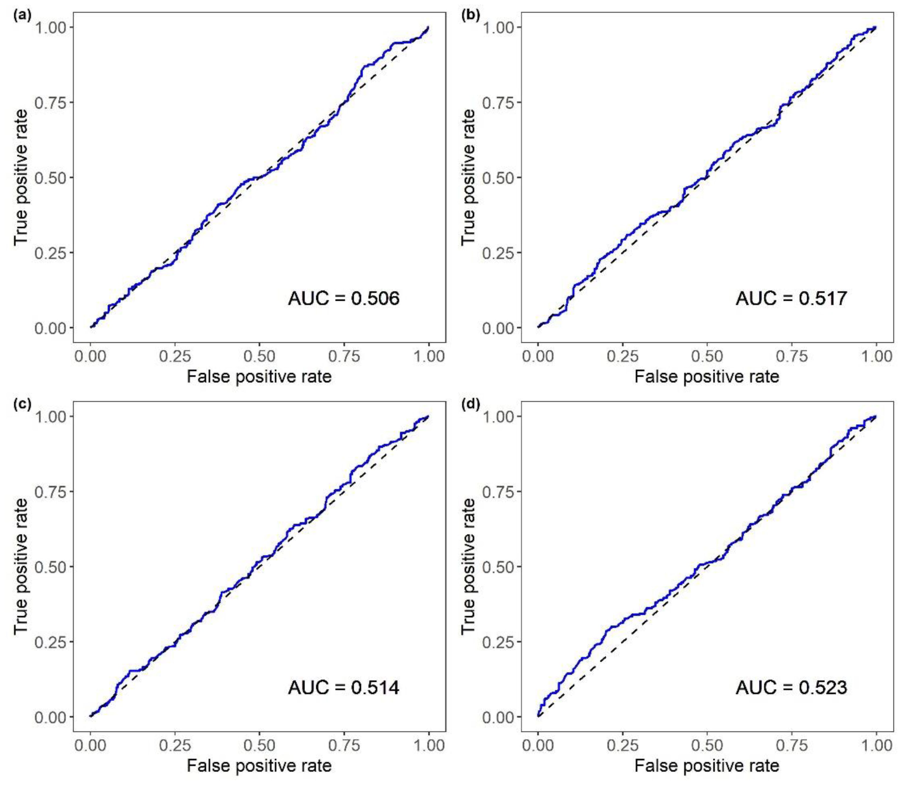
| EBVFH for MORT | BLUP | 0.506 (0.009) | 0.526 (0.005) | 0.090 (0.024) |
| EBVFH for BW | BLUP | 0.517 (0.004) | 0.529 (0.005) | 0.093 (0.009) |
| EBVFH for SRHC | BLUP | 0.514 (0.009) | 0.525 (0.008) | 0.085 (0.017) |
| EBVFH for AT | BLUP | 0.523 (0.005) | 0.534 (0.006) | 0.106 (0.014) |
Publisher’s Note: MDPI stays neutral with regard to jurisdictional claims in published maps and institutional affiliations. |
© 2022 by the authors. Licensee MDPI, Basel, Switzerland. This article is an open access article distributed under the terms and conditions of the Creative Commons Attribution (CC BY) license (https://creativecommons.org/licenses/by/4.0/).
Share and Cite
Faggion, S.; Bertotto, D.; Bonfatti, V.; Freguglia, M.; Bargelloni, L.; Carnier, P. Genomic Predictions of Phenotypes and Pseudo-Phenotypes for Viral Nervous Necrosis Resistance, Cortisol Concentration, Antibody Titer and Body Weight in European Sea Bass. Animals 2022, 12, 367. https://doi.org/10.3390/ani12030367
Faggion S, Bertotto D, Bonfatti V, Freguglia M, Bargelloni L, Carnier P. Genomic Predictions of Phenotypes and Pseudo-Phenotypes for Viral Nervous Necrosis Resistance, Cortisol Concentration, Antibody Titer and Body Weight in European Sea Bass. Animals. 2022; 12(3):367. https://doi.org/10.3390/ani12030367
Chicago/Turabian StyleFaggion, Sara, Daniela Bertotto, Valentina Bonfatti, Matteo Freguglia, Luca Bargelloni, and Paolo Carnier. 2022. "Genomic Predictions of Phenotypes and Pseudo-Phenotypes for Viral Nervous Necrosis Resistance, Cortisol Concentration, Antibody Titer and Body Weight in European Sea Bass" Animals 12, no. 3: 367. https://doi.org/10.3390/ani12030367
APA StyleFaggion, S., Bertotto, D., Bonfatti, V., Freguglia, M., Bargelloni, L., & Carnier, P. (2022). Genomic Predictions of Phenotypes and Pseudo-Phenotypes for Viral Nervous Necrosis Resistance, Cortisol Concentration, Antibody Titer and Body Weight in European Sea Bass. Animals, 12(3), 367. https://doi.org/10.3390/ani12030367