Wild Isolates of Neurospora crassa Reveal Three Conidiophore Architectural Phenotypes


Abstract
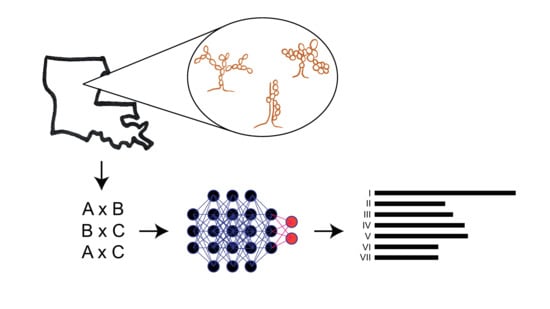
1. Introduction
2. Materials and Methods
2.1. Strains and Media
2.2. Crosses and Progeny Screening
2.3. Microscopy and Image Deconvolution
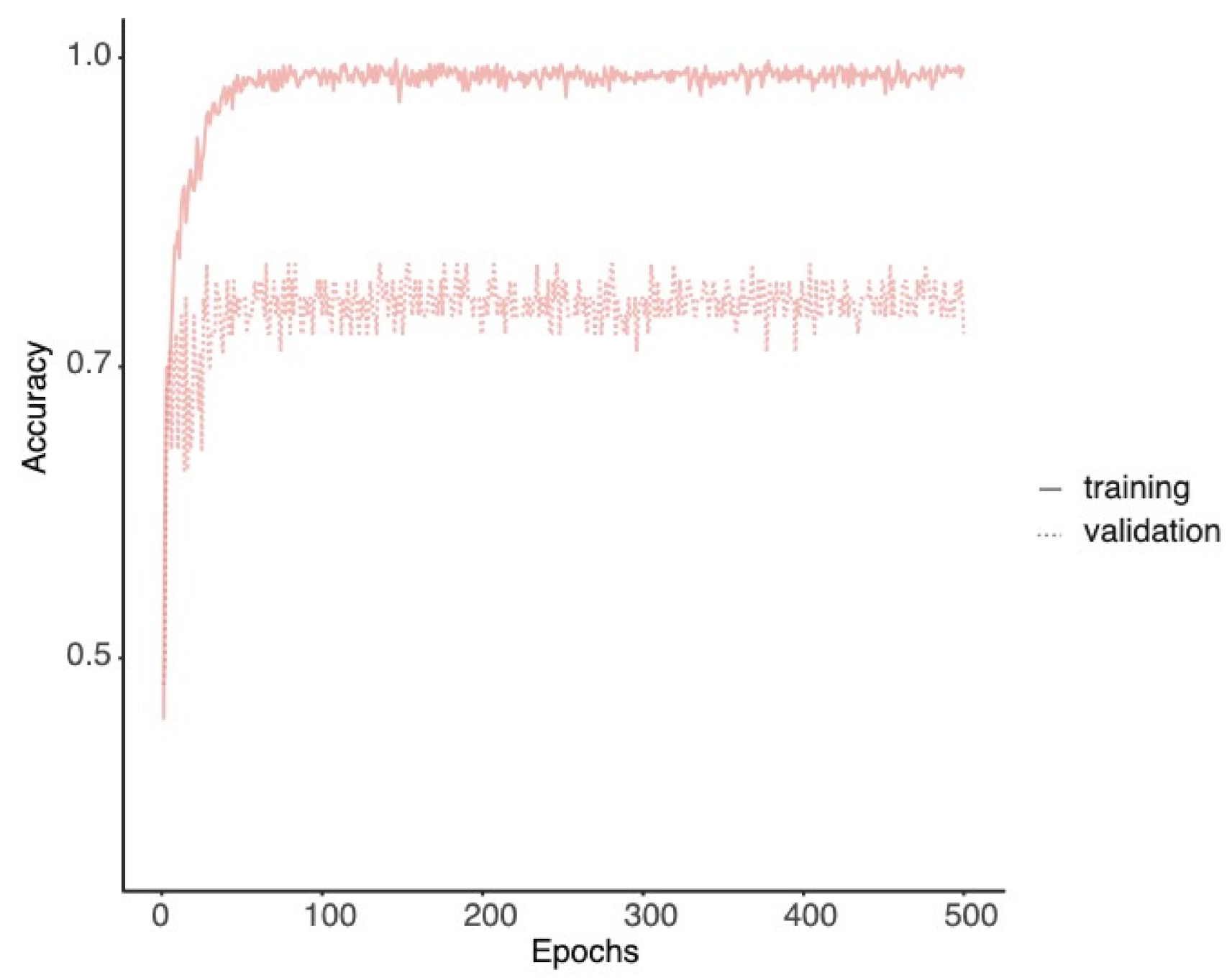
2.4. Automated Phenotype Classification
2.5. Sporulation Quantification
3. Results
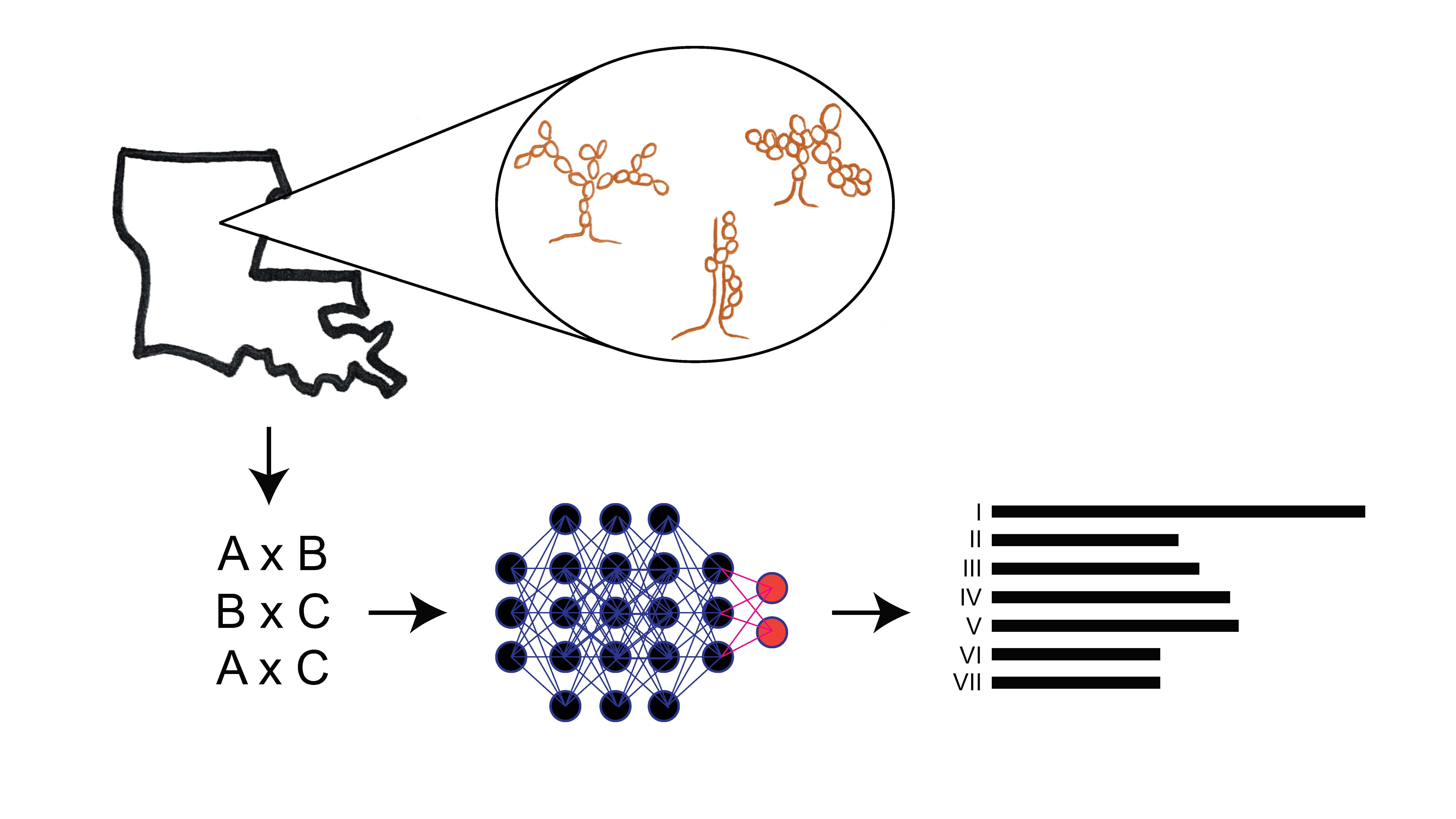
3.1. Wild N. crassa Isolates Exhibit Three Conidiophore Architectural Phenotypes
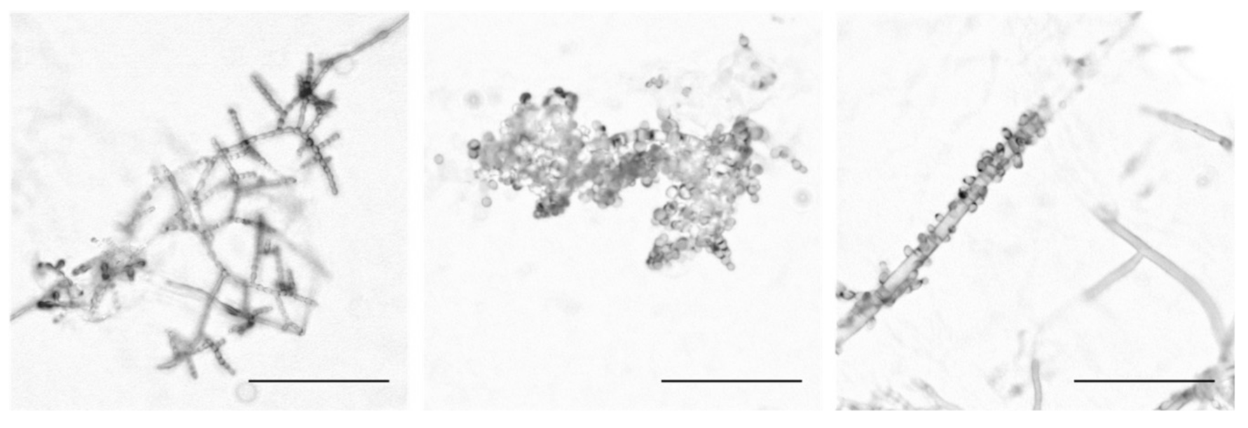
3.2. Architectural Phenotypes Are Consistent throughout Conidiophore Development
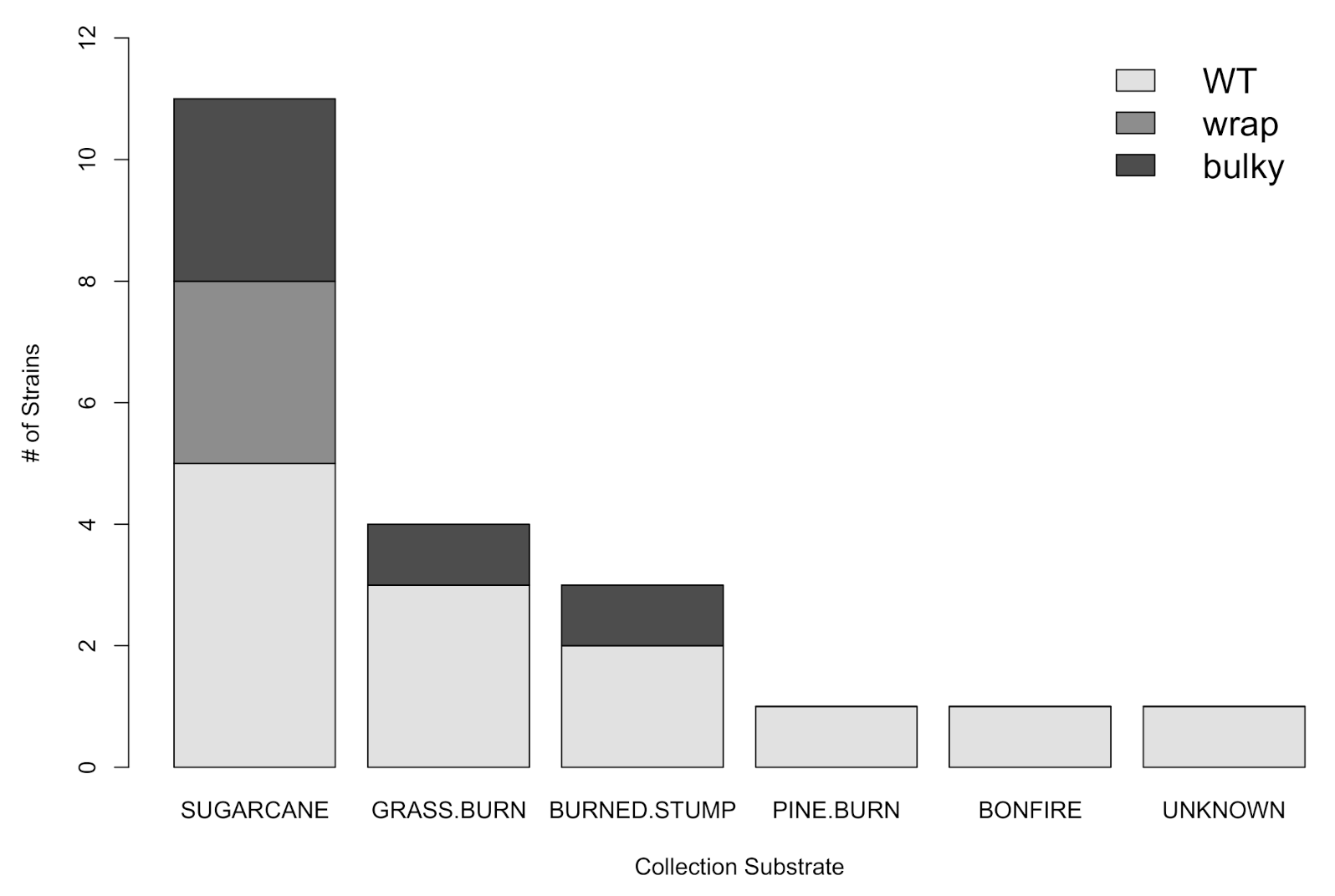
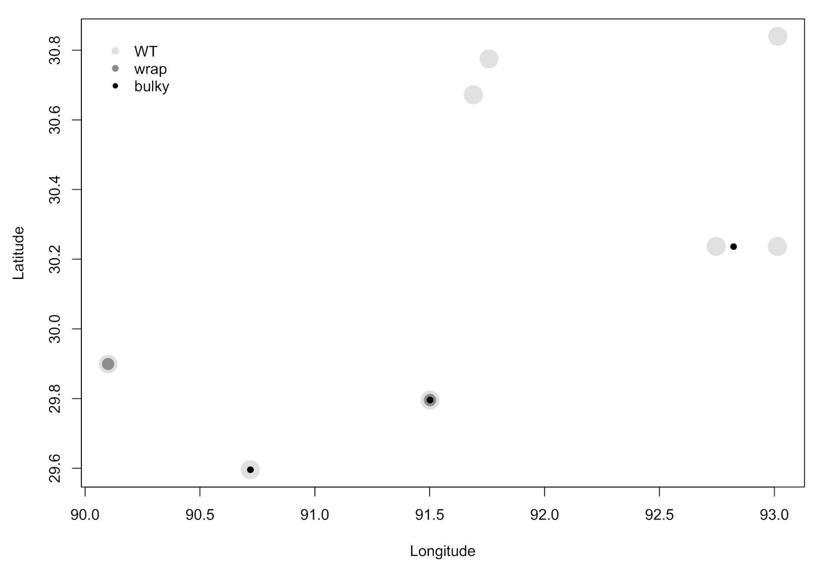
3.3. There Is No Dependence of Phenotype on Strain Collection Environment
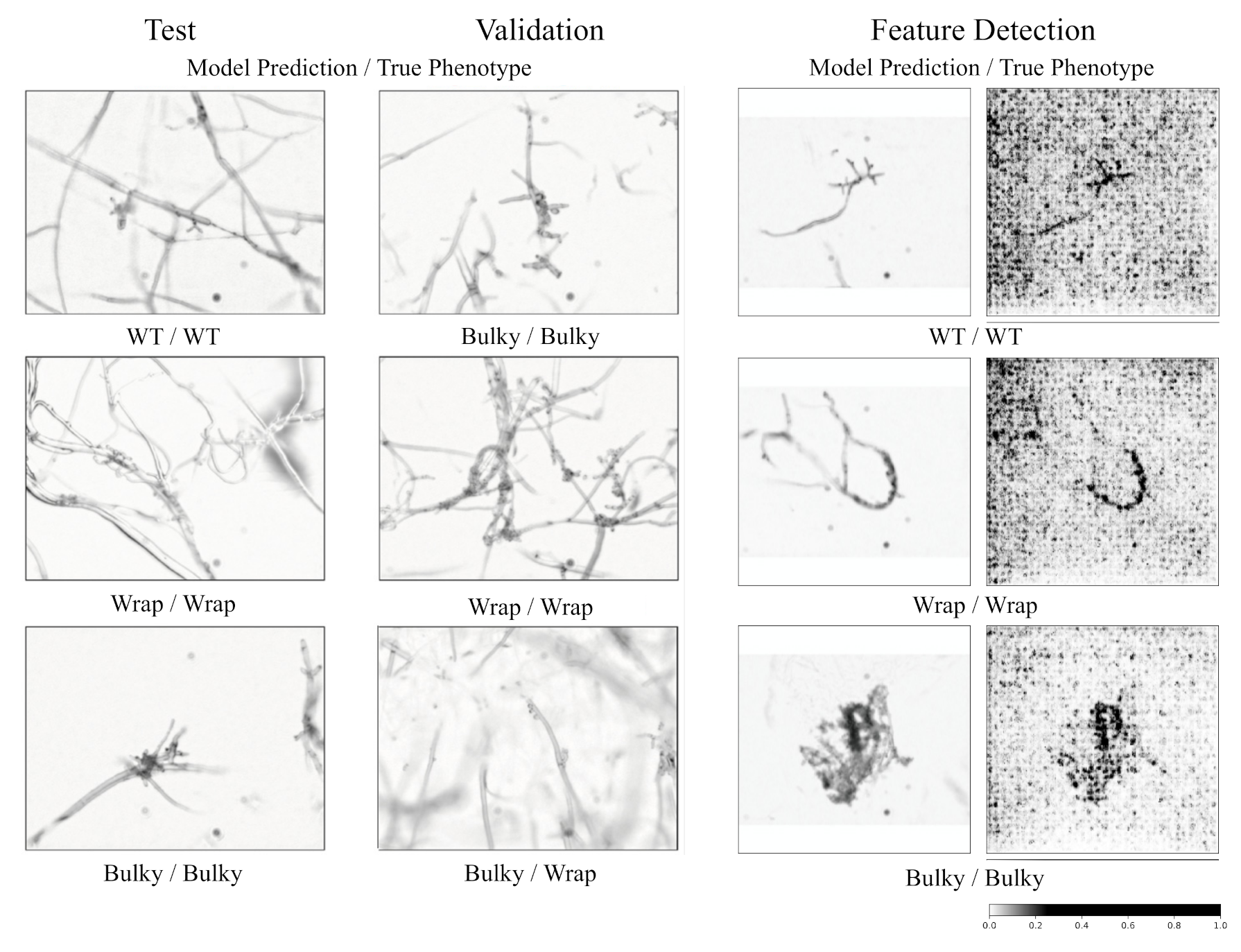
3.4. Architectural Phenotypes Can Be Automatically Classified and Corresponding Features Can Be Extracted
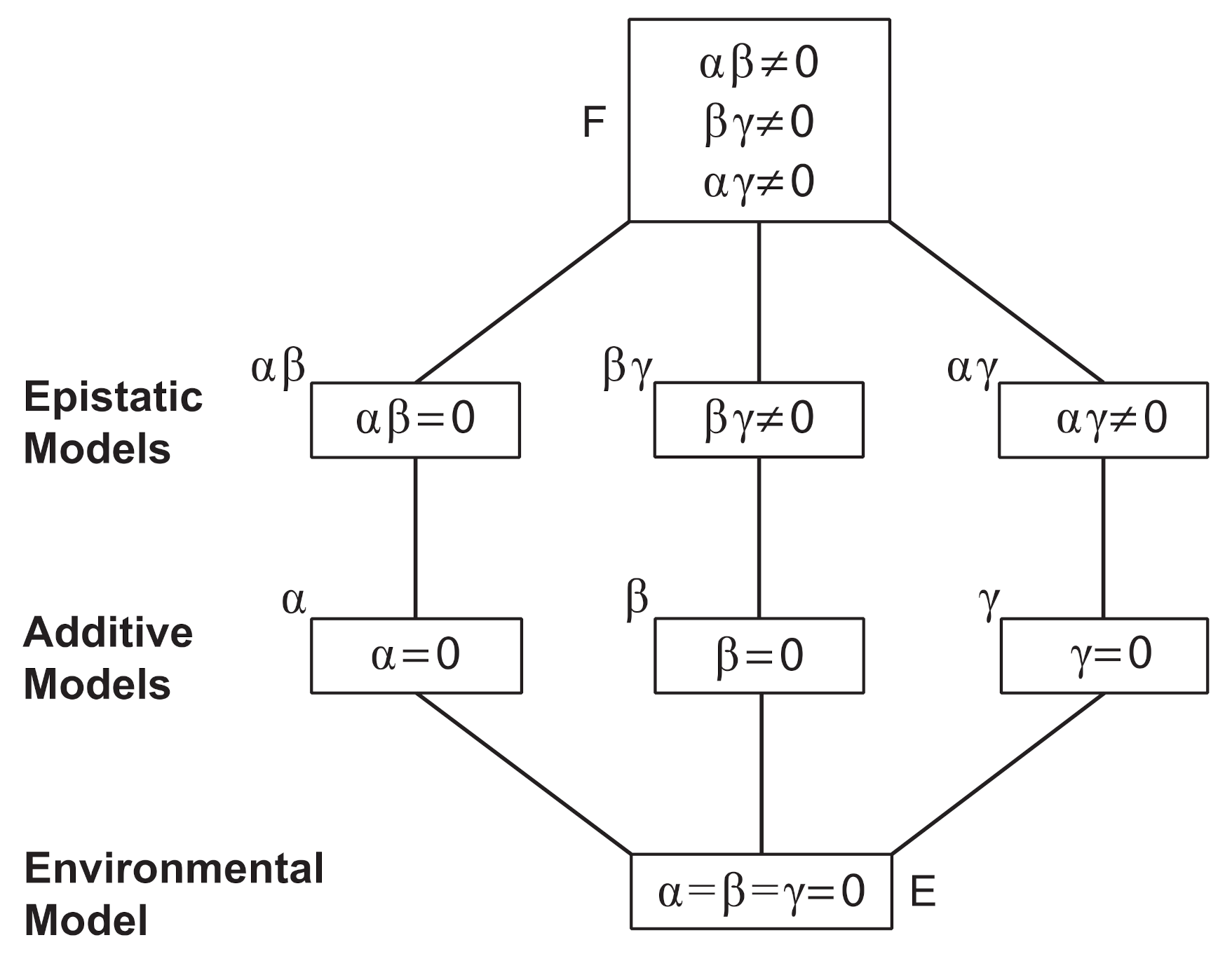
3.5. Crosses Suggest at Least 2–3 Genes Involved in Conidiophore Architectural Phenotypes
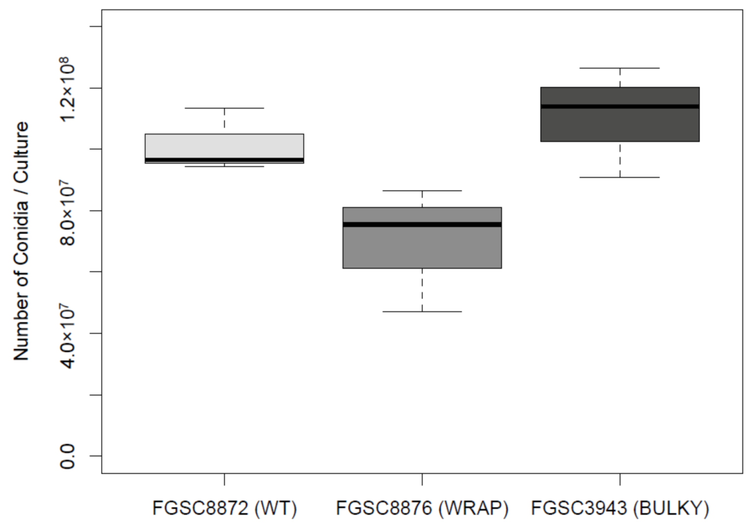
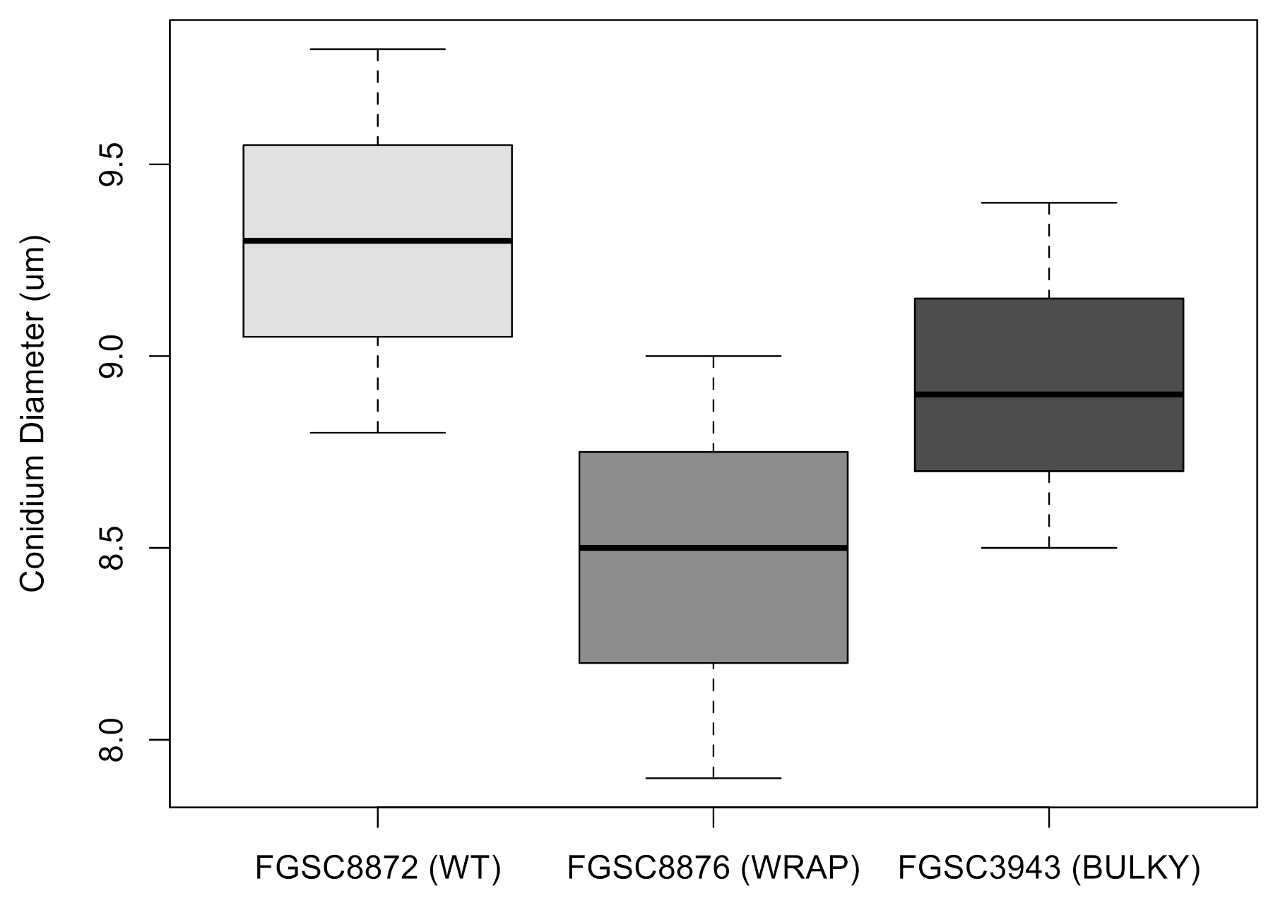
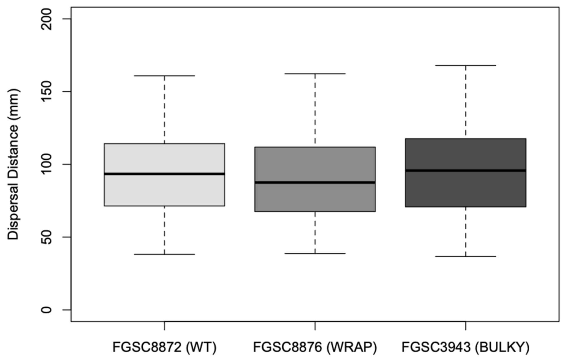
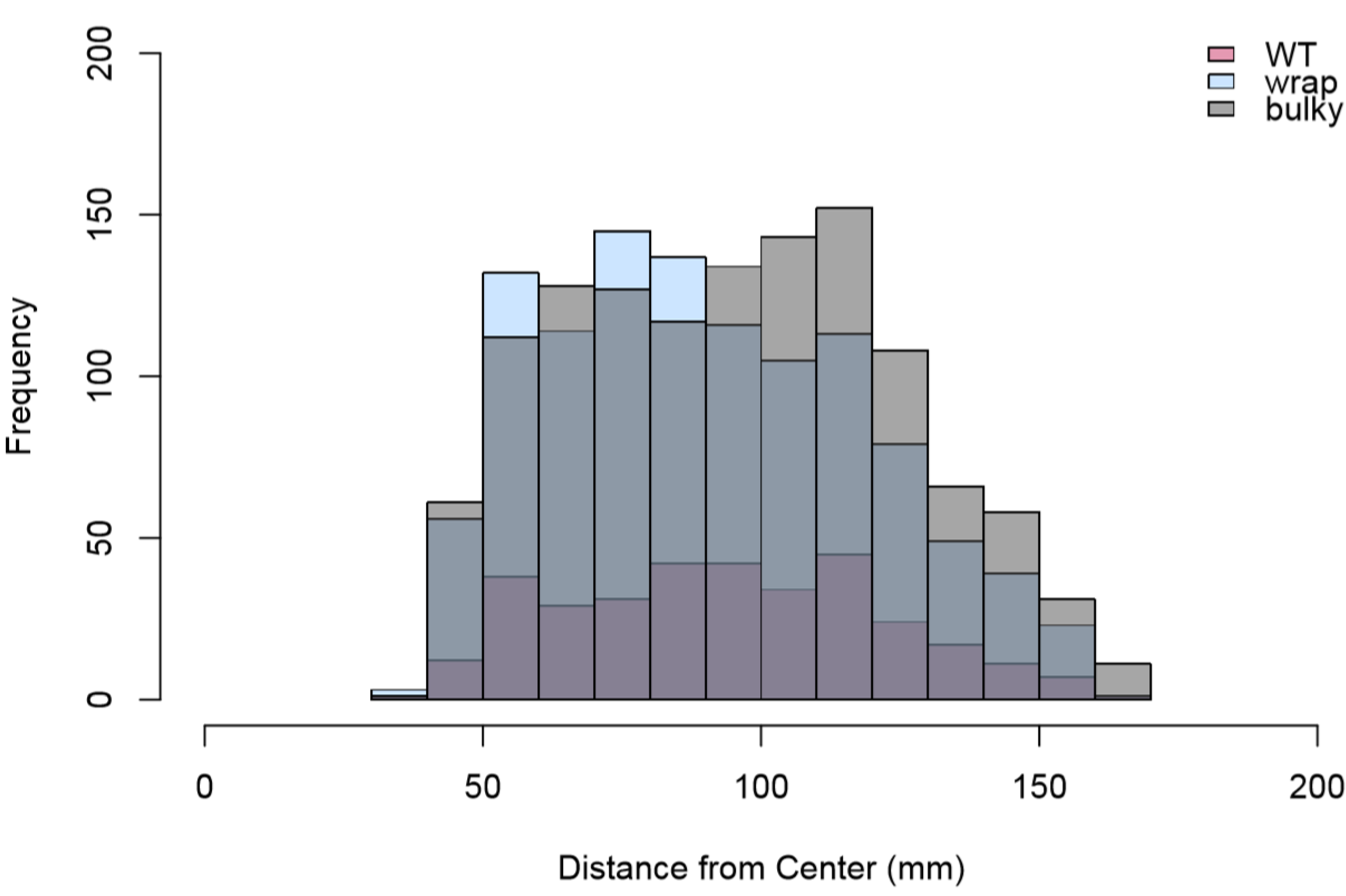
3.6. Architectural Phenotype May Impact Colonization Capacity in N. crassa
4. Discussion
Author Contributions
Funding
Acknowledgments
Conflicts of Interest
Appendix A

| Strain Number | FGSC | Perkins | Mat | Strain Provenance | Collection Site | Substrate/Annotation |
|---|---|---|---|---|---|---|
| Wild Strains | ||||||
| D110 | 8870 | 4448 | A | Dettman, J. | Franklin, LA | sugarcane |
| D111 | 8871 | 4449 | a | Dettman, J. | Franklin, LA | sugarcane |
| D112 | 8872 | 4453 | A | Dettman, J. | Franklin, LA | sugarcane |
| D114 | 8874 | 4464 | A | Dettman, J. | Franklin, LA | sugarcane |
| D116 | 8876 | 4481 | a | Dettman, J. | Franklin, LA | sugarcane |
| D118 | 8878 | 4491 | a | Dettman, J. | Franklin, LA | sugarcane |
| JW09 | 2229 | A | Welch, J. | Welsh, LA | burned grass | |
| JW10 | 2229 | A | Welch, J. | Welsh, LA | burned grass | |
| JW59 | 3200 | a | Welch, J. | Coon, LA | burned stumps | |
| JW66 | 3211 | a | Welch, J. | Sugartown, LA | Pine burn | |
| JW70 | 3199 | A | Welch, J. | Coon, LA | burned stumps | |
| JW75 | 3943 | a | Welch, J. | Houma, LA | sugarcane burn | |
| 847 | A | Lein | Louisiana | sugarcane burn | ||
| D113 | 8873 | 4454 | a | Dettman, J. | Franklin, LA | sugarcane |
| D119 | 8879 | 4500 | a | Dettman, J. | Franklin, LA | sugarcane |
| JW20 | 3212 | A | Welch, J. | Ravenswood, LA | bonfire | |
| JW76 | 3943 | a | Welch, J. | Houma, LA | sugarcane burn | |
| JW159 | 2221 | a | Welch, J. | Houma, LA | sugarcane burn | |
| JW160 | 2222 | A | Welch, J. | Iowa, LA | grass burn | |
| JW162 | 2223 | a | Welch, J. | Iowa, LA | grass burn | |
| JW164 | 2224 | a | Welch, J. | Marrero, LA | wood burn | |
| JW167 | 2228 | a | Welch, J. | Roanoke, LA | grass burn | |
| OR74A | 2489 | A | FGSC | Marrero, LA | unknown | |

References
- Davis, R.H. Contributions of a Model Organism; Oxford University Press: New York, NY, USA, 2000. [Google Scholar]
- Maheshwari, R. Microconidia of Neurospora crassa. Fungal Genet. Biol. 1999, 26, 1–18. [Google Scholar] [CrossRef]
- Sargent, M.L.; Kaltenborn, S.H. Effects of Medium Composition and Carbon Dioxide on Circadian Conidiation in Neurospora. Plant Physiol. 1972, 50, 171–175. [Google Scholar] [CrossRef]
- Springer, M.L.; Yanofsky, C. A morphological and genetic analysis of conidiophore development in Neurospora crassa. Genes Dev. 1989, 3, 559–571. [Google Scholar] [CrossRef]
- Olmedo, M.; Ruger-Herreros, C.; Corrochano, L.M. Regulation by Blue Light of the fluffy Gene Encoding a Major Regulator of Conidiation in Neurospora crassa. Genetics 2009, 184, 651–658. [Google Scholar] [CrossRef]
- Bailey-Shrode, L.; Ebbole, D.J. The fluffy Gene of Neurospora crassa is Necessary and Sufficient to Induce Conidiophore Development. Genetics 2004, 166, 1741–1749. [Google Scholar] [CrossRef]
- Greenwald, C.J.; Kasuga, T.; Glass, N.L.; Shaw, B.D.; Ebbole, D.J.; Wilkinson, H.H. Temporal and Spatial Regulation of Gene Expression During Asexual Development of Neurospora crassa. Genetics 2010, 186, 1217–1230. [Google Scholar] [CrossRef] [PubMed]
- Wang, F.; Dijksterhuis, J.; Wyatt, T.; Wösten, H.A.B.; Bleichrodt, R.-J. VeA of Aspergillus niger increases spore dispersing capacity by impacting conidiophore architecture. Antonie van Leeuwenhoek 2015, 107, 187–199. [Google Scholar] [CrossRef][Green Version]
- Lau, G.W.; Hamer, J.E. Acropetal: A Genetic Locus Required for Conidiophore Architecture and Pathogenicity in the Rice Blast Fungus. Fungal Genet. Biol. 1998, 24, 228–239. [Google Scholar] [CrossRef]
- Mir-Rashed, N.; Jacobson, D.; Dehghany, M.; Micali, O.; Smith, M. Molecular and Functional Analyses of Incompatibility Genes at het-6 in a Population of Neurospora crassa. Fungal Genet. Biol. 2000, 30, 197–205. [Google Scholar] [CrossRef]
- Ellison, C.E.; Hall, C.; Kowbel, D.; Welch, J.; Brem, R.B.; Glass, N.L.; Taylor, J.W. Population genomics and local adaptation in wild isolates of a model microbial eukaryote. Proc. Natl. Acad. Sci. USA 2011, 108, 2831–2836. [Google Scholar] [CrossRef]
- Ellison, C.E.; Kowbel, D.; Glass, N.L.; Taylor, J.W.; Brem, R.B. Discovering Functions of Unannotated Genes from a Transcriptome Survey of Wild Fungal Isolates. mBio 2014, 5, e01046-13. [Google Scholar] [CrossRef]
- Palma-Guerrero, J.; Hall, C.R.; Kowbel, D.; Welch, J.; Taylor, J.W.; Brem, R.B.; Glass, N.L. Genome Wide Association Identifies Novel Loci Involved in Fungal Communication. PLoS Genet. 2013, 9, e1003669. [Google Scholar] [CrossRef]
- He, K.; Zhang, X.; Ren, S.; Sun, J. Deep Residual Learning for Image Recognition. In Proceedings of the 2016 IEEE Conference on Computer Vision and Pattern Recognition, Las Vegas, NV, USA, 27–30 June 2016; pp. 770–778. [Google Scholar]
- McCluskey, K. The Fungal Genetics Stock Center: From Molds to Molecules. Adv. Appl. Microbiol. 2003, 52, 245–262. [Google Scholar] [CrossRef] [PubMed]
- Schneider, C.A.; Rasband, W.S.; Eliceiri, K.W. NIH Image to ImageJ: 25 years of image analysis. Nat. Methods 2012, 9, 671–675. [Google Scholar] [CrossRef]
- Deng, Z.; Arsenault, S.; Caranica, C.; Griffith, J.; Zhu, T.; Al-Omari, A.; Schüttler, H.-B.; Arnold, J.; Mao, L. Synchronizing stochastic circadian oscillators in single cells of Neurospora crassa. Sci. Rep. 2016, 6, 35828. [Google Scholar] [CrossRef]
- Russakovsky, O.; Deng, J.; Su, H.; Krause, J.; Satheesh, S.; Ma, S.; Huang, Z.; Karpathy, A.; Khosla, A.; Bernstein, M.; et al. ImageNet Large Scale Visual Recognition Challenge. Int. J. Comput. Vis. 2015, 115, 211–252. [Google Scholar] [CrossRef]
- Sokolova, M.; Lapalme, G. A systematic analysis of performance measures for classification tasks. Inf. Process. Manag. 2009, 45, 427–437. [Google Scholar] [CrossRef]
- Paszke, A.; Gross, S.; Massa, F.; Lerer, A.; Bradbury, J.; Chanan, G.; Killeen, T.; Lin, Z.; Gimelshein, N.; Antiga, L.; et al. PyTorch: An Imperative Style, High-Performance Deep Learning Library. arXiv 2019, arXiv:1912.01703. [Google Scholar]
- Sundararajan, M.; Taly, A.; Yan, Q. Axiomatic Attribution for Deep Networks. arXiv 2017, arXiv:1703.01365. [Google Scholar]
- Adebayo, J.; Gilmer, J.; Muelly, M.; Goodfellow, I.; Hardt, M.; Kim, B. Sanity Checks for Saliency Maps. In Proceedings of the 32nd Conference on Neural Information Processing Systems (NeurIPS 2018), Montréal, QC, Canada, 3–8 December 2018. [Google Scholar]
- Sturmfels, P.; Lundberg, S.; Lee, S.-I. Visualizing the Impact of Feature Attribution Baselines. Distill 2020, 5, e22. [Google Scholar] [CrossRef]
- Case, M.E.; Griffith, J.; Dong, W.; Tigner, I.L.; Gaines, K.; Jiang, J.C.; Jazwinski, S.M.; Arnold, J. The aging biological clock in Neurospora crassa. Ecol. Evol. 2014, 4, 3494–3507. [Google Scholar] [CrossRef]
- Brunson, J.K.; Griffith, J.; Bowles, D.; Case, M.E.; Arnold, J. lac-1 and lag-1 with ras-1 affect aging and the biological clock in Neurospora crassa. Ecol. Evol. 2016, 6, 8341–8351. [Google Scholar] [CrossRef]
- Falconer, D.S. Introduction to Quantitative Genetics; Longman: London, UK, 1981. [Google Scholar]
- Timberlake, W.E. Molecular Genetics of Aspergillus Development. Annu. Rev. Genet. 1990, 24, 5–36. [Google Scholar] [CrossRef]
- Williams, C.J.E.A. An Analysis of Density-Dependent Viability Selection. J. Am. Stat. Assoc. 1989, 84, 662–668. [Google Scholar] [CrossRef]
- Asmussen, M.A.; Arnold, J.; Avise, J.C. Definition and Properties of Disequilibrium Statistics for Associations between Nuclear and Cytoplasmic Genotypes. Genetics 1987, 115, 755–768. [Google Scholar]
- Kendall, M.; Stuart, A. The Advanced Theory of Statistics. Vol.2: Inference and Relationship; Macmillan: New York, NY, USA, 1979. [Google Scholar]
- Park, H.-S.; Yu, J.-H. Genetic control of asexual sporulation in filamentous fungi. Curr. Opin. Microbiol. 2012, 15, 669–677. [Google Scholar] [CrossRef]
- Turner, B.C.; Perkins, D.D.; Fairfield, A. Neurospora from Natural Populations: A Global Study. Fungal Genet. Biol. 2001, 32, 67–92. [Google Scholar] [CrossRef]
- Berlin, V.; Yanofsky, C. Protein changes during the asexual cycle of Neurospora crassa. Mol. Cell. Biol. 1985, 5, 839–848. [Google Scholar] [CrossRef]
- Perkins, D.D.; Radford, A.; Sachs, M.S. The Neurospora Compendium: Chromosomal Loci; Academic Press: San Diego, CA, USA, 2000. [Google Scholar]
- Powell, J.R.; Dobzhansky, T. How Far Do Flies Fly? The effects of migration in the evolutionary process are approached through a series of experiments on dispersal and gene diffusion in Drosophila. Am. Sci. 1976, 64, 179–185. [Google Scholar]
- Lemke, K. Dispersal Models for Drosophila. Master’s Thesis, Statistics Department, University of Georgia, Athens, GA, USA, 1985. [Google Scholar]
- Powell, A.J.; Jacobson, D.J.; Salter, L.; Natvig, D.O. Variation among natural isolates of Neurospora on small spatial scales. Mycologia 2003, 95, 809–819. [Google Scholar] [CrossRef]
- Galagan, J.E.; Calvo, S.E.; Borkovich, K.A.; Selker, E.U.; Read, N.D.; Jaffe, D.; Fitzhugh, W.; Ma, L.-J.; Smirnov, S.; Purcell, S.; et al. The genome sequence of the filamentous fungus Neurospora crassa. Nat. Cell Biol. 2003, 422, 859–868. [Google Scholar] [CrossRef] [PubMed]
- Judge, M.T.; Wu, Y.; Tayyari, F.; Hattori, A.; Glushka, J.; Ito, T.; Arnold, J.; Edison, A.S. Continuous in vivo Metabolism by NMR. Front. Mol. Biosci. 2019, 6, 26. [Google Scholar] [CrossRef]
- Ohya, Y.; Sese, J.; Yukawa, M.; Sano, F.; Nakatani, Y.; Saito, T.L.; Saka, A.; Fukuda, T.; Ishihara, S.; Oka, S.; et al. High-dimensional and large-scale phenotyping of yeast mutants. Proc. Natl. Acad. Sci. USA 2005, 102, 19015–19020. [Google Scholar] [CrossRef]
- Levy, S.F.; Siegal, M.L. Network Hubs Buffer Environmental Variation in Saccharomyces cerevisiae. PLoS Biol. 2008, 6, e264. [Google Scholar] [CrossRef]
- Das, A.; Schneider, H.; Burridge, J.; Ascanio, A.K.M.; Wojciechowski, T.; Topp, C.N.; Lynch, J.P.; Weitz, J.S.; Bucksch, A. Digital imaging of root traits (DIRT): A high-throughput computing and collaboration platform for field-based root phenomics. Plant Methods 2015, 11, 1–12. [Google Scholar] [CrossRef] [PubMed]
- Parniske, M. Arbuscular mycorrhiza: The mother of plant root endosymbioses. Nat. Rev. Genet. 2008, 6, 763–775. [Google Scholar] [CrossRef]
- Johnson, N.C.; Hoeksema, J.D.; Chaudhary, V.B.; Gehring, C.; Klironomos, J.; Moutoglis, P.; Simard, S.; Swenson, W.; Umbanhowar, J.; Zabinski, C.; et al. From Lilliput to Brobdingnag: Extending Models of Mycorrhizal Function across Scales. Bioscience 2006, 56, 889–900. [Google Scholar] [CrossRef]


| Strain | WT | Bulky | Wrap | Total |
|---|---|---|---|---|
| FGSC0847 | 22 | 0 | 4 | 26 |
| FGSC2221 | 26 | 1 | 3 | 30 |
| FGSC2222 | 13 | 0 | 8 | 21 |
| FGSC2223 | 10 | 2 | 3 | 15 |
| FGSC2224 | 16 | 23 | 6 | 45 |
| FGSC2228 | 39 | 0 | 5 | 44 |
| FGSC2229 | 14 | 54 | 48 | 116 |
| FGSC2489 | 32 | 7 | 1 | 40 |
| FGSC3199 | 17 | 0 | 2 | 19 |
| FGSC3200 | 30 | 5 | 23 | 58 |
| FGSC3211 | 20 | 16 | 7 | 43 |
| FGSC3212 | 54 | 2 | 6 | 62 |
| FGSC3943 | 32 | 80 | 52 | 164 |
| FGSC8870 | 19 | 2 | 9 | 30 |
| FGSC8871 | 16 | 6 | 17 | 39 |
| FGSC8872 | 14 | 0 | 4 | 18 |
| FGSC8873 | 8 | 11 | 13 | 32 |
| FGSC8874 | 20 | 3 | 14 | 37 |
| FGSC8876 | 15 | 21 | 42 | 78 |
| FGSC8878 | 20 | 26 | 12 | 58 |
| FGSC8879 | 6 | 12 | 11 | 29 |
| Total | 443 | 271 | 290 |
| Accuracy | Precision | Recall | |
|---|---|---|---|
| Training | 0.9632 | 0.9644 | 0.9632 |
| Validation | 0.7879 | 0.7890 | 0.7879 |
| Test | 0.7576 | 0.7540 | 0.7576 |
| External test set | 0.6779 | 0.6802 | 0.6639 |
| Bulky | Wrap | WT | |
|---|---|---|---|
| Bulky | 21 | 1 | 0 |
| Wrap | 4 | 13 | 5 |
| WT | 2 | 4 | 16 |
| A (WT) | B (Wrap) | C (Bulky) | |
|---|---|---|---|
| A × B | |||
| B × C | |||
| A × C |
| A (WT) | B (Wrap) | C (Bulky) | |
|---|---|---|---|
| A × B | = 205 | ||
| B × C | = 155 | = 275 | |
| A × C | = 230 | = 198 |
| Parameters/K | |||||||
|---|---|---|---|---|---|---|---|
| 1 | 1 | −1 | 0 | 1 | 0 | 0 | |
| 1 | −1 | 1 | 0 | 1 | 0 | 0 | |
| 1 | −1 | −1 | 0 | −1 | 0 | 0 | |
| 1 | 0 | −1 | −1 | 0 | −1 | 0 | |
| 1 | 0 | 1 | −1 | 0 | 1 | 0 | |
| 1 | 0 | −1 | 1 | 0 | −1 | 0 | |
| 1 | 1 | 0 | −1 | 0 | 0 | 1 | |
| 1 | −1 | 0 | −1 | 0 | 0 | −1 | |
| 1 | −1 | 0 | 1 | 0 | 0 | 1 |
| Model | Χ2 | df | p | X2HA − X2H0 | df | p for HA vs. H0 | Notes |
|---|---|---|---|---|---|---|---|
| Full epistatic | 0.98 | 2 | 0.61 | - | - | - | H0 = full epistatic |
| 8.39 | 3 | 0.04 | 8.39 − 0.98 = 7.41 | 1 | 0.004 | H0 = full epistatic | |
| 25.31 | 5 | 0.001 | 25.31 − 0.98 = 24.33 | 2 | <0.00001 | H0 = full epistatic | |
| 9.96 | 5 | 0.08 | 9.96 − 0.98 = 8.98 | 2 | 0.01 | H0 = full epistatic | |
| 9.32 | 3 | 0.02 | 9.32 − 0.98 = 8.34 | 1 | 0.004 | H0 = full epistatic | |
| 84.57 | 3 | <0.0001 | 84.57 − 0.98 = 83.59 | 1 | <0.00001 | H0 = full epistatic | |
additive | 95.76 | 4 | <0.0001 | 95.76 − 0.98 = 94.78 | 3 | <0.00001 | H0 = full epistatic |
| environmental | 124.46 | 8 | <0.0001 | 124.46 − 0.98 = 123.48 | 7 | <0.00001 | H0 = full epistatic |
| heritability | H2 = (124.46 − 95.76)/124.46 = 0.23 H0 = environmental model H1 = full additive model |
| Parameters | Full Epistatic 3 Genes | 2 Genes |
|---|---|---|
| 5.32 ± 0.0040 | 5.32 ± 0.0030 | |
| −0.08 ± 0.0048 | 0.02 ± 0.0048 | |
| 0.05 ± 0.0061 | 0 | |
| 0.53 ± 0.0047 | 0.53 ± 0.0044 | |
| −0.15 ± 0.0060 | 0 | |
| 0.20 ± 0.0067 | 0.23 ± 0.0061 | |
| −0.60 ± 0.0064 | −0.58 ± 0.0062 |
Publisher’s Note: MDPI stays neutral with regard to jurisdictional claims in published maps and institutional affiliations. |
© 2020 by the authors. Licensee MDPI, Basel, Switzerland. This article is an open access article distributed under the terms and conditions of the Creative Commons Attribution (CC BY) license (http://creativecommons.org/licenses/by/4.0/).
Share and Cite
Krach, E.K.; Wu, Y.; Skaro, M.; Mao, L.; Arnold, J. Wild Isolates of Neurospora crassa Reveal Three Conidiophore Architectural Phenotypes. Microorganisms 2020, 8, 1760. https://doi.org/10.3390/microorganisms8111760
Krach EK, Wu Y, Skaro M, Mao L, Arnold J. Wild Isolates of Neurospora crassa Reveal Three Conidiophore Architectural Phenotypes. Microorganisms. 2020; 8(11):1760. https://doi.org/10.3390/microorganisms8111760
Chicago/Turabian StyleKrach, Emily K., Yue Wu, Michael Skaro, Leidong Mao, and Jonathan Arnold. 2020. "Wild Isolates of Neurospora crassa Reveal Three Conidiophore Architectural Phenotypes" Microorganisms 8, no. 11: 1760. https://doi.org/10.3390/microorganisms8111760
APA StyleKrach, E. K., Wu, Y., Skaro, M., Mao, L., & Arnold, J. (2020). Wild Isolates of Neurospora crassa Reveal Three Conidiophore Architectural Phenotypes. Microorganisms, 8(11), 1760. https://doi.org/10.3390/microorganisms8111760