On-Line Modal Parameter Identification Applied to Linear and Nonlinear Vibration Absorbers

Abstract

A solution of the vibration attention problem on a flexible structure from a dynamic vibration absorption perspective is experimentally and numerically studied in this article. Linear and nonlinear dynamic vibration absorbers are properly implemented on a primary structure of n degrees of freedom through a modal decomposition analysis and using the tuning condition when the primary system has one single degree of freedom. A time-domain algebraic identification scheme for on-line modal parameter estimation of flexible structures is presented. A fast frequency estimation of harmonic excitation force is also obtained. A Hilbert transform analysis of the frequency response function for the case of nonlinear dynamic vibration absorption is introduced. In this way, influence of this particular passive nonlinear control device on system dynamic response can be determined. The proposed approach is validated on an harmonically perturbed building-like structure, which is discretized in a finite number of degrees of freedom. The flexible structure is subjected to resonant operational conditions, and coupled to a pendulum vibration absorber configured as a tuned mass damper as well as an autoparametric system.

1. Introduction

It is well known that excessive vibrations represent a destructive dynamic condition. Repetitive operation or external forces cause simultaneous movement that can resonate through the machine, building or bridge to a dangerous magnitude. One common method to address the vibration control issue on flexible mechanical structures is through linear or nonlinear passive devices, taking advantage of the physical properties of the system itself. In order to prevent undesirable consequences of vibrations, this method modifies, mostly, mass, damping and stiffness properties with regard to initial configuration of the principal structure. Passive control techniques are characterized by implementation of devices in structures that do not require any external energy source to reduce mechanical vibrations [1,2].

Within the approach of linear passive vibration control, one of the widely used devices is the tuned mass damper (TMD), which consists of a mass, a spring and a viscous damper. This device is frequently implemented because of its properties such as effectiveness, reliability and low costs, with applications such as machinery and civil structures [3].

TMD was initially used at the beginning of the past century since its conceptualization was applied for the first time by Frahm to reduce movement of ships as well as vibrations of the ships hull [4]. After a major development on its dynamic behavior, TMD was designed to control the structural dynamic response on different topics. Ormondroyd and Den Hartog [5] came upon that a TMD, with a damping element, can suppress the amplitude of the primary system in a wider frequency range, followed by a detailed discussion of the optimization that adjusts the damping parameters. Application of a passive vibration control scheme in flexible structures, using a TMD, is not just for controlling the dynamic response on lateral loads but also to mitigate torsional displacements in buildings with significant torsional coupling [6].

Simplicity of tuned mass dampers makes them the most used devices for vibration control in buildings with great height. Guo and Chen [7] proposed an innovative technique for using multiple TMDs to control partial loads on the ground in a limited number of floors. They indicated using numerical results that the use of multiple TMDs can effectively alter the distribution of natural frequencies as well as reduce the frequency/transient responses of the structure. Nowadays, research related to the study and implementation of a TMD remains a current topic, for example, for vibration control of adjacent twin buildings or using it in combination with the tapering method in order to control the dynamic response of super-tall buildings [8,9].

However, the use of nonlinear devices for passive vibration control is a relevant issue due to dynamic behaviors that may occur and do not happen in linear vibration systems [10]. Usually, a nonlinear vibration absorber is implemented in order to overcome possible drawbacks due to the use of a TMD [11]. There is a classification of nonlinear vibration absorbers called autoparametric absorbers. This type of nonlinear systems differ from the traditional TMD, mainly because these have nonlinear coupling between at least two vibration modes, satisfying the so-called autoparametric condition (external and internal resonance condition), which are certainly related with parametric excitation. Autoparametric absorbers are specifically used where a primary system is being excited close to one of its principal parametric resonances—that is, the worst case situation in a physical structure. When the autoparametric interaction occurs between two subsystems, there is a great energy transfer to the autoparametric absorber.

Autoparametric absorbers have been designed to mitigate resonant oscillations due to the advantages that this type of systems present in their frequency response function in comparison with the classic vibration absorber (TMD). Ibrahim and Heo [12] and Dahlberg [13] described how a continuous cantilever beam absorber with tip mass, oriented in the same direction with the motion of the primary system, can be implemented with better attenuation properties than those obtained with classical TMD. Cuvalci et al. [14] defined an absorption region for an autoparametric vibration absorber for a single degree of freedom primary system under sinusoidal and random excitations. They experimentally determined the parameters that influence the effectiveness of a nonlinear vibration absorber. Hui and Ng [15] presented the implementation of autoparametric phenomena to reduce symmetrical vibration of a curved beam/panel under external harmonic excitation showing that internal energy transfer of a first symmetric mode into first anti-symmetric mode in a curved panel is one example of autoparametric vibration absorber effect. Abundis-Fong et al. [16] developed an optimum design of an autoparametric absorber (cantilever beam configuration) coupled to a resonant oscillator where the implementation of the nonlinear absorber was obtained by using an approximation of the nonlinear frequency response function, computed via a perturbation method. Recently, Ting Tan et al. [17] used the nonlinear saturation principle and 1:2 internal resonance in the design of the piezoelectric autoparametric vibration absorber for vibration suppression and energy harvesting. Moreover, active vibration absorbers can be implemented to suppress undesirable vibrations and simultaneous tracking of reference trajectories by implementing on-line algebraic parameter identification methods [18]. In this paper, the theoretical framework for algebraic parametrical identification of linear dynamical systems introduced in [19] is extended to the on-line modal parameter estimation problem of a class of harmonically perturbed flexible structures. It has been theoretically proved that algebraic identification is robust against noise and polynomial disturbances. On-line algebraic identification has been also applied for synthesis of model-free control strategies [20] and numerical differentiation techniques of noisy measurement signals [21].

In this article, we are interested in implementing an on-line modal parameters identification technique to two different passive vibration control schemes for a flexible structure, justifying its tuning by means of a modal decomposition, in order to make an experimental comparison from a dynamic, frequency and energy approach. The work is structured as follows. In Section 2, the tuning conditions of the passive control schemes implemented are required. The dynamic representation and modal decomposition of a flexible structure with n degrees of freedom are presented in Section 3. In Section 4 an on-line algebraic identification scheme for estimating the amplitude and frequency of a harmonic excitation is detailed. Experiments using linear (TMD) and nonlinear (autoparametric system) vibration absorber for a flexible structure discretized in a finite number of degrees of freedom are presented in Section 5. Finally, conclusions are given in Section 6.

2. Preliminaries

This section briefly reviews, in a general way, the tuning conditions of a linear absorber (TMD) and a nonlinear one (autoparametric type) for the case of a primary system with a single degree of freedom.

2.1. Linear Vibration Absorber: Tuned Mass Damper

A TMD is a mechanical device to be added to another mechanical system, often called the primary system, with the purpose of attenuating unwanted vibrations by introducing equal and opposite dynamics forces or by damping devices to dissipate energy. Its effectiveness depends on the closeness of absorber’s natural frequency to the excitation frequency. Basically, a conventional TMD consists of a single mass connected to the main structure by a linear spring and a viscous damper. Therefore, the most representative model for a structure with a TMD is a two degrees of freedom system, whose vibratory dynamics is described by the two coupled ordinary differential equations

$$\begin{array}{ccc}\hfill m_1{\ddot{x}}_1+c_1{\dot{x}}_1+(k_1+k_a)x_1-k_a{x}_2& =& F\left(t\right)\hfill \end{array}$$

(1)

$$\begin{array}{ccc}\hfill m_a{\ddot{x}}_2+c_a{\dot{x}}_2-k_a\left(x_1-x_2\right)& =& 0\hfill \end{array}$$

(2)

where $m_1$, $c_1$ and $k_1$ represent mass, damping and stiffness parameters of the primary system. TMD parameters are denoted by $m_a$, $c_a$ and $k_a$. The harmonic force is described by $F\left(t\right)=F_{0}sin{\Omega }t$ with amplitude $F_0$ and excitation frequency ${\Omega }$. For a primary system with a single degree of freedom, it is possible to tune a TMD in order to passively control the first resonant vibration mode [22]. In general, design parameters of the vibration absorber ($m_a$ and $k_a$) should be selected such as its uncoupled natural frequency ${\omega }_{n2}$ is close to the excitation force frequency ${\Omega }$; this is,

$${\omega }_{n2}={\Omega }=\sqrt{\frac{k_a}{m_a}}$$

(3)

In this way, passive suppression of the harmonic excitation force can be performed as depicted in Figure 1. Moreover, for a realistic primary system we have that $c_1>0$, global asymptotic stability can be hence achieved by the passive vibration control device [18]. Additional viscous damping $c_a$ can be properly added into a passive vibration absorber to increase the attenuation band around its tuning frequency [23]. Robustness against variations on the excitation frequency ${\Omega }$ can be thus improved.

2.2. Nonlinear Vibration Absorber: Autoparametric System

A functional passive vibration absorber extracts oscillatory energy from the primary system. This type of energy transfer is well established in autoparametric vibration. In the simplest case, an autoparametric system can be thought in two parts, the first being an externally excited forced oscillator and the second comprising an oscillator parametrically (a term appears as a time varying modification of a system parameter) excited by the response of the forced element.

The coupling between vibration modes (either two or more) is the fundamental requirement of an autoparametric system in such a way that response relationships can be made to apply between the natural frequencies and also the frequency of external excitation [24]. An autoparametric system can be modelled in a general sense (considering two degrees of freedom) by the following normalized equations of motion

$$\begin{array}{ccc}\hfill \ddot{x}+2{\zeta }_1{\omega }_1\dot{x}+{\omega }_1^{2}x-\epsilon \mu ({\dot{y}}^2+y\ddot{y})& =& F_{0}sin{\Omega }t\hfill \end{array}$$

(4)

$$\begin{array}{ccc}\hfill \ddot{y}+2{\zeta }_2{\omega }_2\dot{y}+{\omega }_2^{2}y-\epsilon \ddot{x}y& =& 0\hfill \end{array}$$

(5)

where x and y are the degrees of freedom associated with the primary system and the autoparametric absorber, respectively. The coupling between Equations (4) and (5) is apparent in the terms $\epsilon \mu ({\dot{y}}^2+y\ddot{y})$ and $\epsilon \ddot{x}y$ where $\epsilon \mu$ and $\epsilon$ are constants related to the properties of the nonlinear absorber to be considered as well as the equivalent mass present in the complete system [24,25]. It is important to note that (5) is clearly a parametric type equation where $\ddot{x}$ acts as a coefficient of the coordinate y.

However, according to the tuning condition between an autoparametric vibration absorber and a mechanical oscillator, the following expressions must be satisfied (for more details see [16])

$$\begin{array}{ccc}\hfill {\Omega }& =& {\omega }_1\hfill \end{array}$$

(6)

$$\begin{array}{ccc}\hfill {\omega }_1& =& 2{\omega }_2\hfill \end{array}$$

(7)

where ${\Omega }$ is the excitation frequency, ${\omega }_1$ is the natural frequency of the main system and ${\omega }_2$ corresponds to the natural frequency of the secondary system. Equations (6) and (7) are known as the external and internal resonance conditions, respectively [26].

Basically, the main feature of autoparametric resonance is the energy transfer when the lower mode frequency is equal to one-half of the higher mode frequency (see (6) and (7)). Because of energy transfer, the lower mode could result in exponential energy growth and may act as a nonlinear vibration absorber to the higher mode.

3. A Flexible Structure with n Degrees of Freedom

Real flexible structures are continuous elastic systems which have an infinite number of degrees of freedom. Therefore, their dynamical analysis commonly entails an approximation. This consists of describing their dynamical behaviour through the use of a finite number of degrees of freedom, as many as necessary to ensure enough accuracy. Flexible structures are usually described as discretized multiple degree-of-freedom systems.

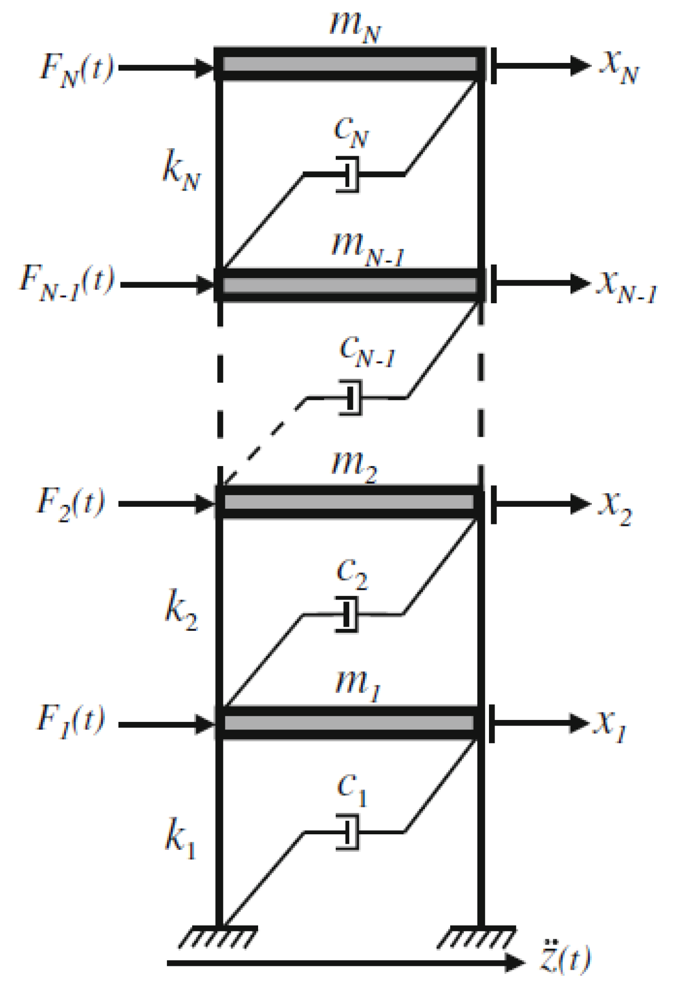
In this work, the primary or main system is composed of a flexible structure which simulates a building-like structure with n degrees of freedom as depicted in Figure 2. Dynamical system behavior can be described by [27]

$$M\ddot{x}+C\dot{x}+Kx=f\left(t\right)$$

(8)

where $x\in R^n$ represents the relative displacement vector with respect to a main frame reference. $M,C$, and K are $n\times n$ matrices of mass, damping and stiffness of the primary system. $f\in R^n$ is the input force vector such that $f={[F_n\left(t\right),F_{n-1}\left(t\right),\cdots ,F_1\left(t\right)]}^T$. It is possible to transform the effect of the ground acceleration, $\ddot{z}\left(t\right)\in R$, as a force acting on each mass by using the vector $e={\left[1,1,\dots ,1\right]}^T\in R^n$. In order to express the forces acting on the system in a compact way, let us define:

$$f\left(t\right)=-Me\ddot{z}\left(t\right)$$

(9)

Substitution of (9) into (8) leads to the linear model of a vibrating mechanical system with n degrees of freedom with base excitation

$$M\ddot{x}+C\dot{x}+Kx=-Me\ddot{z}\left(t\right)$$

(10)

A linear or nonlinear dynamic vibration absorber can be then connected over the nth floor of the primary system for passive vibration control purposes. The main objective is to decrease harmonic oscillations disturbing a specific vibration mode, near some natural frequency of the main system.

Primary system (10) can be then expressed in terms of modal or principal coordinates $q_i\left(t\right),i=1,2\dots ,n$ as follows [28,29]

$${\ddot{q}}_i+2{\zeta }_i{\omega }_{ni}{\dot{q}}_i+{\omega }_{ni}^2{q}_i={\mathsf{\Psi }}^{T}f$$

(11)

with

$$x\left(t\right)=\mathsf{\Psi }q\left(t\right)$$

(12)

where $q\left(t\right)\in R^n$ stands for a vector of modal or principal coordinates. $f\in R^n$ represents an external force vector. Parameters ${\zeta }_i$ and ${\omega }_{ni}$ are the equivalent modal damping and the natural frequency. $\mathsf{\Psi }$ is the $n\times n$ modal matrix given by

$$\mathsf{\Psi }=\left[\begin{array}{ccc}{\psi }_{11}& \dots & {\psi }_{1n}\\ ⋮& \ddots & ⋮\\ {\psi }_{n1}& \dots & {\psi }_{nn}\end{array}\right]$$

(13)

The mathematical model of the flexible structure (10) can be hence described as

$${\ddot{q}}_i+2{\zeta }_i{\omega }_{ni}{\dot{q}}_i+{\omega }_{ni}^2{q}_i={\psi }_{1i}{f}_1+\cdots +{\psi }_{ni}{f}_n$$

(14)

Using notation of operational calculus of Mikusiński [28,30], modal model (14) can be also written as

$$\left(s^2+2{\zeta }_i{\omega }_{ni}s+{\omega }_{ni}^2\right)q_i\left(s\right)={\psi }_{1i}{f}_1\left(s\right)+\cdots +{\psi }_{ni}{f}_n\left(s\right)+c_{0,i}+c_{1,i}s$$

(15)

with $s=j\omega$, $j=\sqrt{-1}$. Modal coordinates $q_i\left(s\right)$ can be then expressed as

$$q_i\left(s\right)=\frac{{\psi }_{1i}{f}_1\left(s\right)+\cdots +{\psi }_{ni}{f}_n\left(s\right)+c_{0,i}+c_{1,i}s}{\left(s^2+2{\zeta }_i{\omega }_{ni}s+{\omega }_{ni}^2\right)}$$

(16)

where constants $c_{0,i}$ and $c_{1,i}$ depend on unknown initial conditions of the system at $t=t_0\ge 0$. From Equations (11) and (12), displacements $x_i$ can be also expressed in notation of operational calculus as

$$x_i\left(s\right)=\sum _{j=1}^n\frac{{\psi }_{ij}{\psi }_{ji}{f}_j\left(s\right)+{\psi }_{ij}(c_{1,i}s+c_{0,i})}{(s^2+2{\zeta }_j{\omega }_{nj}s+{\omega }_{nj}^2)}$$

(17)

This representation leads to the expression

$$p_c\left(s\right)x_i\left(s\right)=\sum _{j=1}^n{\beta }_i\left(s\right)\left[{\psi }_{ij}{\psi }_{ji}{f}_j\left(s\right)+{\psi }_{ij}(c_{1,i}s+c_{0,i})\right]$$

(18)

with

$${\beta }_i\left(s\right)=s^{2n-1}+b_{(2n-2)i}{s}^{2n-2}+\dots +b_{1i}s+b_{0i}$$

(19)

$$p_c\left(s\right)=s^{2n}+a_{2n-1}{s}^{2n-1}+\cdots a_2{s}^2+a_{1}s+a_0$$

(20)

where $p_c\left(s\right)$ is an unique polynomial independent of the output variable $x_i$ available for parametrical estimation. Furthermore, $p_c\left(s\right)$ is known as the characteristic polynomial of the dynamical system. Here, $b_{ji}$ are constants that depend on the roots of $p_c\left(s\right)$. Roots of the characteristic polynomial (20) provide the natural frequencies and damping ratios of the flexible structure.

Equation (11) describes the dynamic characteristics of the ith vibration mode and it constitutes what is known as the modal model, i.e., this describes the system through its modal properties (mode shapes, natural frequencies, and damping ratios), as opposed to the spatial model (10), where the system is described by its spatial properties (M, C, and K) [3,29].

Once the original system (10) has been decoupled by (11) and (12), it is possible to focus on the vibration mode to be attenuated or damped. Therefore, passive vibration control on the flexible mechanical structure converges to the primary system configuration of a single degree of freedom with a secondary system (vibration absorber). The vibration absorption device can be tuned to the original system either using (3), for the linear case, or (6) and (7) for the nonlinear case (autoparametric absorber). It is important to mention that although the vibration absorber is tuned to attenuate a single vibration mode, in fact, it is capable of attenuating the dynamic response of all degrees of freedom of the primary flexible structure. This situation is shown in the experimental results section of the present study.

4. Time-Domain and On-Line Algebraic Identification of the Harmonic Excitation

Consider the mechanical system shown in Figure 2 with a dynamic behavior described by the mathematical model (10). It is possible to use measurements of a single position variable $x_i$ in the synthesis of a modal model based on coefficients $a_k$ of the characteristic polynomial (20) [30,31]. When the ground acceleration produces the excitation force $f\left(t\right)$ as described in (8), individual component forces $F_i$ are harmonic. We can then express those forces in notation of operational calculus as follows

$$F_i\left(s\right)=m_i{{\Omega }}_0^{2}A\frac{{{\Omega }}_0^2}{s^2+{{\Omega }}_0^2}$$

(21)

where the frequency ${{\Omega }}_0$ and the amplitude A is the same for each component of the input force vector $f_k$. Hence, by substituting (21) in (18) we have:

$$p_c\left(s\right)x_i\left(s\right)=\sum _{j=1}^n{\beta }_i\left(s\right)\left[{\psi }_{ij}{\psi }_{ji}{m}_i{{\Omega }}_0^{2}A\frac{{{\Omega }}_0^2}{s^2+{{\Omega }}_0^2}+{\psi }_{ij}(c_{1,i}s+c_{0,i})\right]$$

(22)

where $p_c\left(s\right)$ is the polynomial defined by (20). Multiplying (22) by $\left(s^2+{{\Omega }}_0^2\right)$ we obtain:

$$\left(s^2+{{\Omega }}_0^2\right)p_c\left(s\right)x_i\left(s\right)=\left(s^2+{{\Omega }}_0^2\right)\sum _{j=1}^n{\beta }_i\left(s\right)\left[{\psi }_{ij}{\psi }_{ji}{m}_i{{\Omega }}_0^{2}A\frac{{{\Omega }}_0^2}{s^2+{{\Omega }}_0^2}+{\psi }_{ij}(c_{1,i}s+c_{0,i})\right]$$

(23)

$$\left(s^{2n+2}+a_{2n-1}{s}^{(2n+2)-1}+a_{2n-2}{s}^{(2n+2)-2}+\cdots +a_1{s}^3+a_0{s}^2\right)x_i\left(s\right)=-{{\Omega }}_0^2{p}_c\left(s\right)+R\left(s\right)$$

(24)

with $R\left(s\right)={\gamma }_0+{\gamma }_1{s}^2+\cdots +{\gamma }_{2n}{s}^{2n+1}$. Constants ${\gamma }_k$, $k=0,1,\dots ,2n$, depend on the modal matrix entries ${\psi }_{ij}$, the mass $m_i$ of each floor and the initial conditions. Then, we derive $2n+2$ times Equation (24) with respect to the variable s in order to annihilate the polynomial disturbance $R\left(s\right)$. Next, the result is multiplied by $s^{-(2n+2)}$ and transformed back to the time domain to yield

$$\nu \left(t\right)={{\Omega }}_0^2\kappa \left(t\right)$$

(25)

where

$$\nu \left(t\right)=v_{2n}\left(t\right)+a_{2n-1}{v}_{2n-1}\left(t\right)+\cdots +a_1{v}_1\left(t\right)+a_0{v}_0\left(t\right)$$

(26)

$$\kappa \left(t\right)=k_{2n}\left(t\right)+a_{2n-1}{k}_{2n-1}\left(t\right)+\cdots +a_1{k}_1\left(t\right)+a_0{k}_0\left(t\right)$$

(27)

with

$$\begin{array}{cc}\hfill v_{2n}\left(t\right)=& \sum _{k=0}^{\mathcal{N}}{\left(-1\right)}^{\mathcal{N}-k}\frac{\mathcal{N}{!}^2}{k!\left(\mathcal{N}-k\right){!}^2}{\int }_{t_0}^{\left(k\right)}\Delta t^{\mathcal{N}-k}{x}_i\left(t\right)\hfill \\ \hfill v_{2n-1}\left(t\right)=& \sum _{k=0}^{\mathcal{N}-1}{\left(-1\right)}^{\mathcal{N}-k}\frac{\mathcal{N}!\left(\mathcal{N}-1\right)!}{k!\left(\mathcal{N}-k\right)!\left(\mathcal{N}-1-k\right)!}{\int }_{t_0}^{(k+1)}\Delta t^{\mathcal{N}-k}{x}_i\left(t\right)\hfill \\ \hfill ⋮& ⋮\hfill \\ \hfill v_1\left(t\right)=& \sum _{k=0}^1{\left(-1\right)}^{\mathcal{N}-k}\frac{\mathcal{N}!}{k!\left(\mathcal{N}-k\right)!(1-k)!}{\int }_{t_0}^{\left(k\right)}\Delta t^{\mathcal{N}-k}{x}_i\left(t\right)\hfill \\ \hfill v_0\left(t\right)=& {\int }_{t_0}^{\mathcal{N}}\Delta t^{\mathcal{N}}{x}_i\left(t\right)\hfill \\ \\ \hfill k_{2n}\left(t\right)=& \sum _{k=0}^{2n}{\left(-1\right)}^{2n-k}\frac{\mathcal{N}!\left(2n\right)!}{k!\left(\mathcal{N}-k\right)!\left(\mathcal{N}-2-k\right)!}{\int }_{t_0}^{\left(k\right)}\Delta t^{2n-k}{x}_i\left(t\right)\hfill \\ \hfill k_{2n-1}\left(t\right)=& \sum _{k=0}^{2n-1}{\left(-1\right)}^{2n-k}\frac{\mathcal{N}!(2n-1)!}{k!\left(\mathcal{N}-k\right)!\left(\mathcal{N}-1-k\right)!}{\int }_{t_0}^{(k+1)}\Delta t^{2n-k}{x}_i\left(t\right)\hfill \\ \hfill ⋮=& \hfill & \hfill ⋮\\ \hfill k_1\left(t\right)=& \sum _{k=0}^1{\left(-1\right)}^{2n-k}\frac{\mathcal{N}!}{k!\left(\mathcal{N}-k\right){!}^2}{\int }_{t_0}^{\left(k\right)}\Delta t^{2n-k}{x}_i\left(t\right)\hfill \\ \hfill k_0\left(t\right)=& {\int }_{t_0}^{\mathcal{N}}\Delta t^{2n}{x}_i\left(t\right)\hfill \end{array}$$

Here, $\mathcal{N}=2n+2$, $\Delta t=t-t_0$, and notation ${\int }_{t_0}^{\left(m\right)}\Phi \left(t\right)$ is employed to represent iterated integrals of the form

$${\int }_{t_0}^t{\int }_{t_0}^{{\sigma }_1}\cdots {\int }_{t_0}^{{\sigma }_{m-1}}\Phi \left({\sigma }_m\right)d{\sigma }_m\cdots d{\sigma }_1$$

(28)

where m is a positive integer. By considering that ${{\Omega }}_0^2$ is a positive number, we have that

$$\left|\nu \left(t\right)\right|{{\Omega }}_0^2=\left|\kappa \left(t\right)\right|$$

(29)

Then, we get an expression for on-line and time-domain estimation of the excitation frequency ${{\Omega }}_0$. It is possible to avoid singularities and, at the same time, to get a considerably smoother estimation by integrating Equation (25) two times respect to time as follows

$${\widehat{{\Omega }}}_0=\sqrt{\frac{{\nu }_I\left(t\right)}{{\kappa }_I\left(t\right)}},t>t_0$$

(30)

with

$${\nu }_I\left(t\right)=e^{-\alpha \Delta t}{\int }_{t_0}^{\left(2\right)}\left|\nu \left(t\right)\right|,{\kappa }_I\left(t\right)=e^{-\alpha \Delta t}{\int }_{t_0}^{\left(2\right)}\left|\kappa \left(t\right)\right|$$

(31)

where $e^{-\alpha \Delta t}$ is used like a low pass filter with cut frequency defined by the parameter $\alpha >0$. In this way, the numerical estimation process implementation of the frequency of the excitation force is smoothed.

The proposed identification scheme is capable to identify the frequency of the excitation force, by using measurements of some of the outputs $x_i$ with a similar performance. In addition, estimation of the parameter ${\widehat{{\Omega }}}_0$ does not depend, neither on the amplitude A of the ground acceleration nor the unknown system initial conditions. Moreover, since measurement noise could be considered as fast external fluctuations corrupting output signals $x_i$, iterated integrals operate like low pass filters [19,32]. In this sense, on-line algebraic identification is, at some extent, robust against noise [19,20,21]. However, measurement signals should be suitably conditioned and pre-filtered to reduce harmful noise levels. Otherwise, for operational scenarios where highly large noise is manifested, a considerable degradation on the estimation performance could occur.

Analysis Based on the Hilbert Transformation

The time-domain and on-line identification scheme is based on the assumption of an approximate linear behavior of the main structure around its nominal operating conditions. Since the on-line identification of the excitation frequency of the structure depends on the validity or precision of the characteristic polynomial (20), it is necessary to have a method or index that indicates the presence of nonlinearities in the vibrational response of the structure and its effect on its dynamic behavior. For nonlinearity analysis purposes, we propose to apply the Hilbert transformation $H_T$ to the frequency response function (FRF) of the system. The Hilbert transformation of a particular FRF is given by [33]

$$H_T\left\{FRF\left(j\omega \right)\right\}=-\frac{1}{\pi }pv{\int }_{-\infty }^{\infty }\frac{FRF\left(j\omega \right)}{j\omega -j{\omega }_c}dj\omega$$

(32)

where the term $pv$ is the Cauchy principal value of the integral. This principal value is necessary since there is a singularity at $j\omega =j{\omega }_c$ in the integrand. Consider that when applying the Hilbert transform to a $FRF\left(j\omega \right)$, which is complex valued, the real part and the imaginary part of $FRF\left(j\omega \right)$ are related by the expressions:

$$\mathrm{Real} \left(FRF\left(j\omega \right)\right) = H_T \left\{\mathrm{Real} \left(FRF\left(j\omega \right)\right)\right\}$$

(33)

$$\mathrm{Im} \left(FRF\left(j\omega \right)\right) = -H_T \left\{\mathrm{Imag} \left(FRF\left(j\omega \right)\right)\right\}$$

(34)

Relations (33) and (34) are known as the Hilbert transformation pairs [33]. This is only valid for linear systems. As a consequence, for nonlinear systems the Hilbert transform will return a distorted version of the original FRF. Therefore, by using these properties of the Hilbert transform we have a nonlinearity indicator determined by quantifying the distortion on the original FRF under the action of the Hilbert transformation operator. For this particular purpose, we calculate the cross correlation coefficient:

$${\eta }_{Hi}={∥R_{H_{T}F}\left(0\right)∥}^2$$

(35)

where $∥R_{H_{T}F}\left(0\right)∥$ is the normalized cross correlation coefficient. The numerical value of ${\eta }_{Hi}$ is used as a nonlinearity index. The complex valued function $FRF\left(j\omega \right)$ is the original FRF of the system and $H_T$ is the Hilbert transformation of $FRF\left(j\omega \right)$, hence, the cross correlation coefficient $R_{H_{T}G}$ is given by

$$R_{H_{T}F}\left(\Delta j\omega \right)={\int }_{-\infty }^{\infty }{H}_T\left(j\omega \right)FRF\left(j\omega +\Delta j\omega \right)dj\omega$$

(36)

The index (35) acts as an indicator of the presence and effects of nonlinearity in a particular vibrating mechanical system at some specific operation condition. In this work, we use this index to determine the level of nonlinear dynamic behavior present in the building-like structure. Since the Hilbert transformation, in an experimental context, is inherently numerical, we need to specify a concrete linearity criteria. Hence, as reported in [28], it is recommended to consider a value of $0.9\le {\eta }_{Hi}\le 1.0$ for an assumption of approximate linear dynamic behavior of the system.

5. Experimental Results

A series of experiments were performed considering two different case studies. A six-story building-like structure discretized in six degrees of freedom with a linear vibration absorber is first implemented. The other case is a different structure discretized in three degrees of freedom on which a nonlinear vibration absorber is implemented. Both of the structures are made of aluminum alloy and supported by columns of the same material.

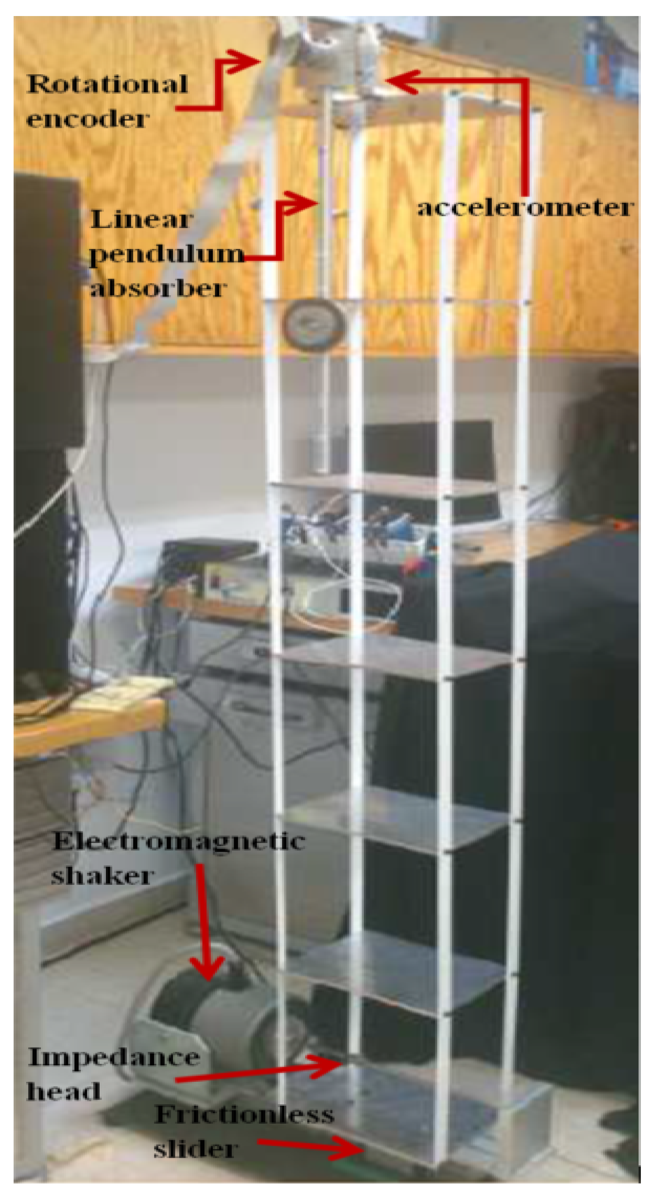
The first primary system to be considered is the six-story building-like structure shown in Figure 3. The sensing elements are IEPE accelerometers attached to each story of the structure and a high resolution rotary encoder used to take angle measurements of the linear pendulum absorber. An electromechanical shaker acts as a source of excitation in conjunction with the frictionless slider for performing experimental modal analysis and performance tests of the vibrations absorber. The impedance head is used to measure the force input, these measurements are needed for the application of experimental modal analysis techniques.

Modal parameters of the structure are obtained using experimental modal analysis, by averaging two of the most popular excitation techniques: impact hammer and sine sweep [28,29]. We then process the corresponding acceleration measurements by applying a FRF-based multiple degrees-of-freedom method (MDoF) [29]. In particular, we apply the well founded RFP curve fitting method described in [34], that is, we express the experimental FRF in terms of rational fraction polynomials so the coefficients $a_k$ of the characteristic polynomial (20) can be determined. The transfer function or estimated FRF for one measurable degree of freedom of the structure can be expressed as a function of the complex variable s, so that:

$${\alpha }_i\left(s\right)=\frac{s^m+{\widehat{b}}_m{s}^{m-1}+\cdots +{\widehat{b}}_2{s}^2+{\widehat{b}}_{1}s+{\widehat{b}}_0}{s^{2n}+{\widehat{a}}_{2n-1}{s}^{2n-1}+\cdots +{\widehat{a}}_2{s}^2+{\widehat{a}}_{1}s+{\widehat{a}}_0}$$

(37)

where $m=2n-2$. Then, the curve fitting method RFP leads to an estimated or fitted FRF (37) such that:

$$e_i\left(s\right)=x_i\left(s\right)-{\alpha }_i\left(s\right)\approx 0$$

(38)

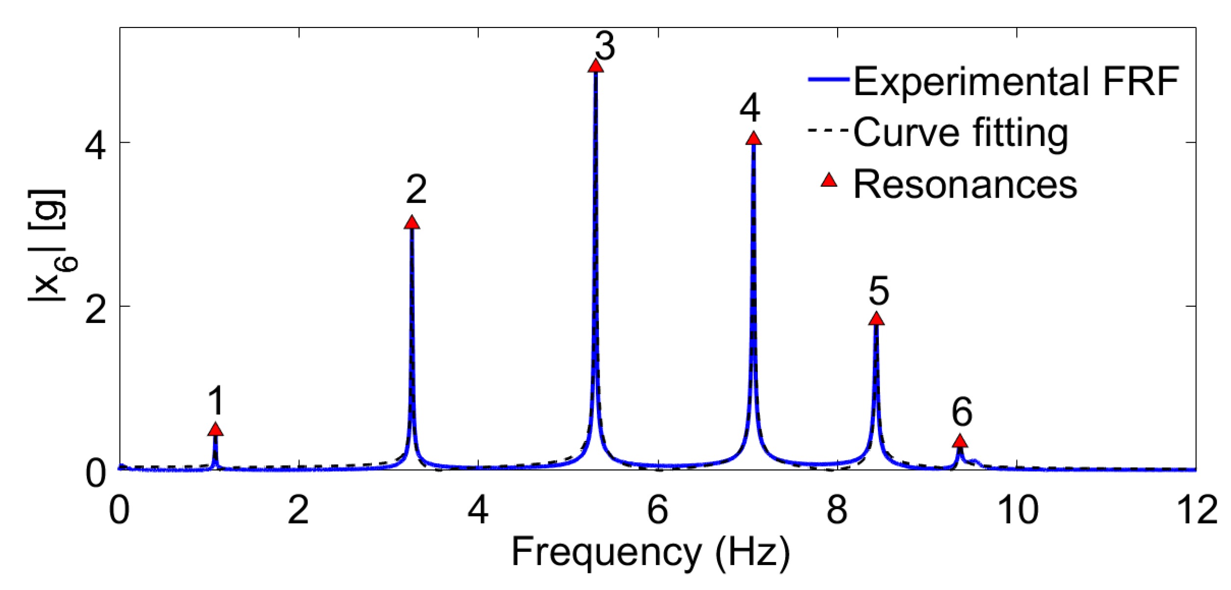
where $e_i\left(s\right)$ is the difference or error between the measured FRF and the estimated FRF, which is constructed by using the coefficients ${\widehat{a}}_k$ and ${\widehat{b}}_k$, $x_i\left(s\right)$ is defined by Equations (17) and (18). The description of the technical details of the curve fitting method are explained in [35]. The experimental and fitted frequency response functions for the primary system is described in Figure 4, where the peaks shown correspond only to transverse vibration modes. We use only measurements of the sixth floor of the structure to apply the curve fitting method. Notice the close relation between the experimental FRF (in solid blue line) and the estimated FRF (in dotted black line) especially near the peaks or resonances. The modal parameters, frequency and damping ratios, obtained by solving the roots of the estimated characteristic polynomial or the denominator of (37) are reported in

Table 1. Modal parameters of the six-story building-like structure.

Mode	Frequency [Hz]	Damping Ratio %
1	1.148	0.15
2	3.39	0.39
3	5.44	0.18
4	7.16	0.19
5	8.53	0.18
6	9.34	0.17

.

The coefficients of the characteristic polynomial are reported in

Table 2. Estimated coefficients of the characteristic polynomial.

Coefficient	Value
${\widehat{a}}_{11}$	1.736
${\widehat{a}}_{10}$	254.8
${\widehat{a}}_9$	345
${\widehat{a}}_8$	$2.408\times {10}^4$
${\widehat{a}}_7$	$2.417\times {10}^4$
${\widehat{a}}_6$	$1.03534\times {10}^6$
${\widehat{a}}_5$	$7.1273\times {10}^5$
${\widehat{a}}_4$	$1.97956\times {10}^7$
${\widehat{a}}_3$	$8.331231\times {10}^6$
${\widehat{a}}_2$	$1.357123\times {10}^8$
${\widehat{a}}_1$	$2.72123\times {10}^7$
${\widehat{a}}_0$	$1.45834\times {10}^8$

. Those coefficients are used for synthesis of an on-line algebraic identifier (30) for the harmonic excitation force.

Then, the characteristic polynomial of the system is

$$p_c\left(s\right)=s^{12}+{\widehat{a}}_{11}{s}^{11}+\cdots +{\widehat{a}}_2{s}^2+{\widehat{a}}_{1}s+{\widehat{a}}_0$$

(39)

where the constants ${\widehat{a}}_k$ are those reported in Table 2.

5.1. Non-Linearity Analysis

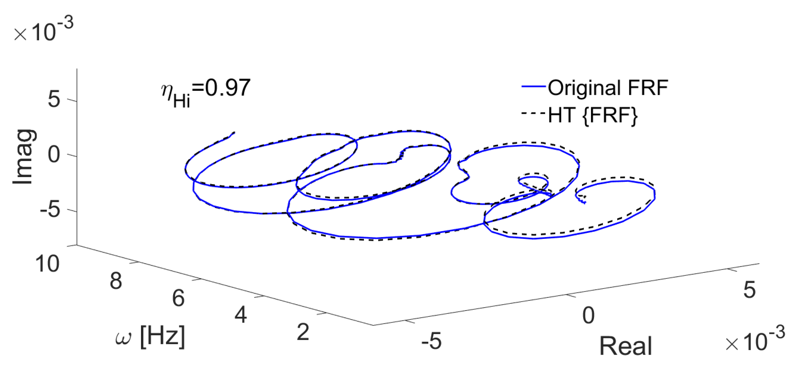
In order to determine the presence of nonlinearities in the dynamic behavior of the six-story building-like structure, we apply an analysis of the frequency response shown in Figure 4. Thus, the non-linearity index defined by (35) is determined. The Nyquist diagram in Figure 5 shows the comparison between the original FRF in solid blue line and the corresponding Hilbert transformation in dotted lines. The numerical value of the calculated no-linearity index is

$${\eta }_{Hi}={∥R_{H_{T}F}\left(0\right)∥}^2=0.97$$

(40)

Therefore, it is assumed that the dynamic behavior of the six-story building structure is dominantly linear and the experimental determination of the coefficients ${\widehat{a}}_k$ of the characteristic polynomial are valid and reliable for the synthesis of the algebraic identifier for the excitation frequency. Moreover, this linear behavior adds a foundation to the reliability of the estimated modal parameters.

5.2. Application of a Linear Absorber

The primary system mentioned above is coupled to a pendulum vibration absorber (configured to work as a TMD) on the top floor. In order to excite the complete system, an electromechanical shaker is used as shown in Figure 3.

Equations of motions related to the system depicted in Figure 3 which is discretized in seven degrees of freedom, considering small angular displacements in the secondary system and submitted to an harmonic forced excitation, are given by

$$\begin{array}{ccc}\hfill M\ddot{x}+C\dot{x}+Kx+\varphi \left(\theta ,\dot{\theta },\ddot{\theta }\right)& =& BF\left(t\right)\hfill \end{array}$$

(41)

$$\begin{array}{ccc}\hfill m_a\ddot{\theta }+c_a\dot{\theta }+k_a\theta +\psi (\ddot{x},\theta )& =& 0\hfill \end{array}$$

(42)

where $x={\left[x_1,x_2,x_3,x_4,x_5,x_6\right]}^T$ is a vector containing the lateral displacements of each floor, $\theta$ is the angular displacement of the pendulum absorber. The mass, damping and stiffness matrices are represented by M, C and K, respectively. The input vector is $B={\left[1,\cdots ,1\right]}^T\in R^6$. According to (9), the input force $F\left(t\right)$ is given by:

$$F\left(t\right)=-\ddot{z}\left(t\right){\left[m_1,m_2,m_3,m_4,m_5,m_6\right]}^T$$

(43)

where $\ddot{z}\left(t\right)$ is the second derivative of ground motion with respect to time. The functions $\varphi \left(\theta ,\dot{\theta },\ddot{\theta }\right)$ and $\psi (\ddot{x},\theta )$ are:

$$\varphi \left(\theta ,\dot{\theta },\ddot{\theta }\right)=\left[\begin{array}{c}0\\ 0\\ ⋮\\ -m_{a}L\theta {\ddot{x}}_6\end{array}\right],\psi (\ddot{x},\theta )=-m_{a}L\theta {\ddot{x}}_6$$

(44)

Parameters associated with the pendulum absorber are its mass ($m_a$), length (L) as well as viscous damping ($c_a$). In the experiments, the base of the structure is directly affected by a ground motion $z\left(t\right)=A_{0}sin\left({\Omega }t\right)$ with amplitude $A_0$ and excitation frequency ${\Omega }$. Due to we are interested in attenuating the first transverse vibration mode, the value of ${\Omega }$ is close to the first resonance frequency ${\omega }_1$. According to (3), the linear pendulum vibration absorber must be tuned in such a way that

$${\Omega }={\omega }_a=\sqrt{g{L}^{-1}}\cong {\omega }_1$$

(45)

Usually, under stable operating conditions, the linear pendulum vibration absorber can be appropriately designed to passively control any vibration mode associated to ${\omega }_i$ ($i=1,2,\dots ,6$) of the main system, depending on the narrow frequency bandwidth where ${\Omega }$ is acting.

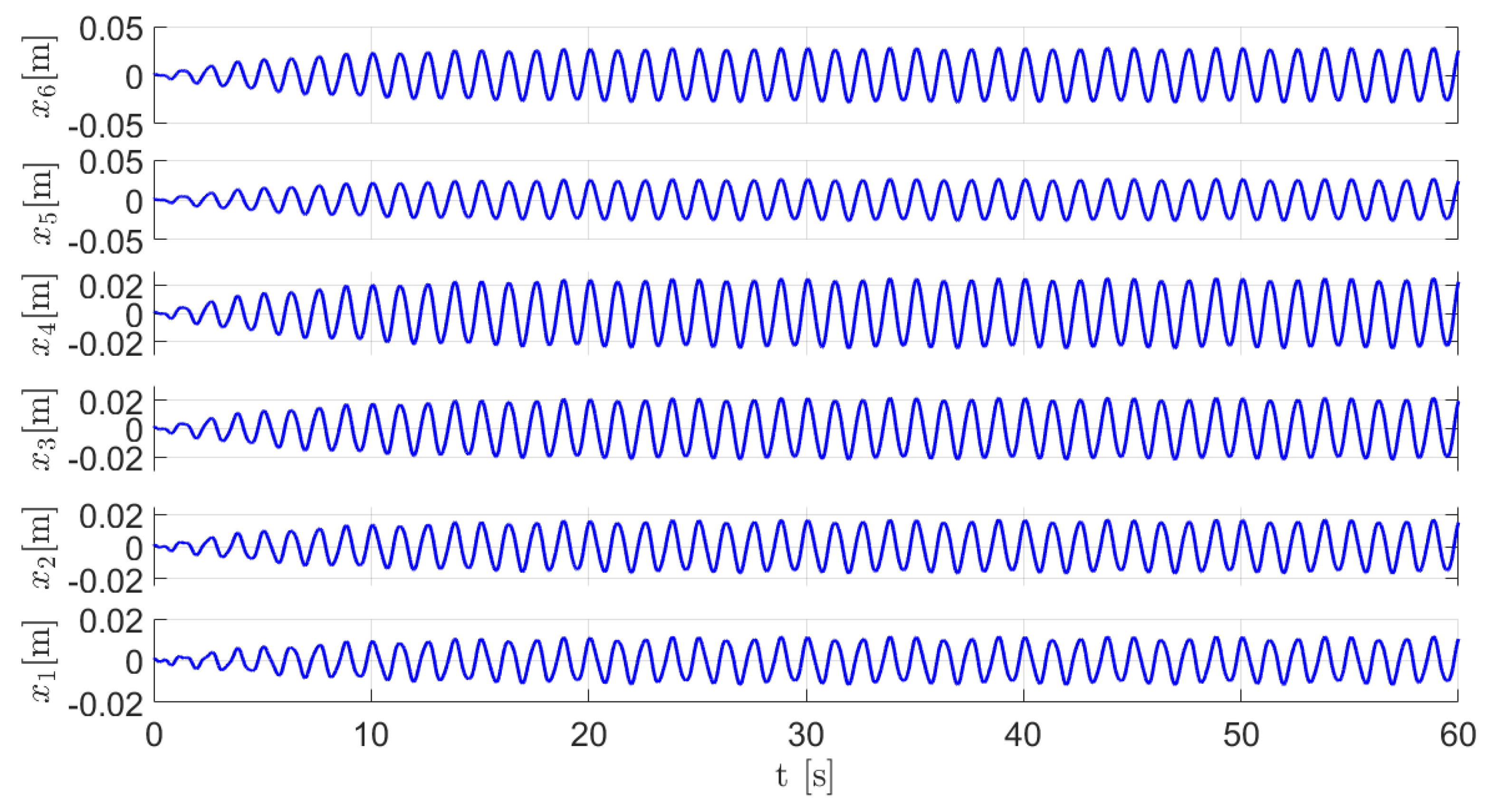
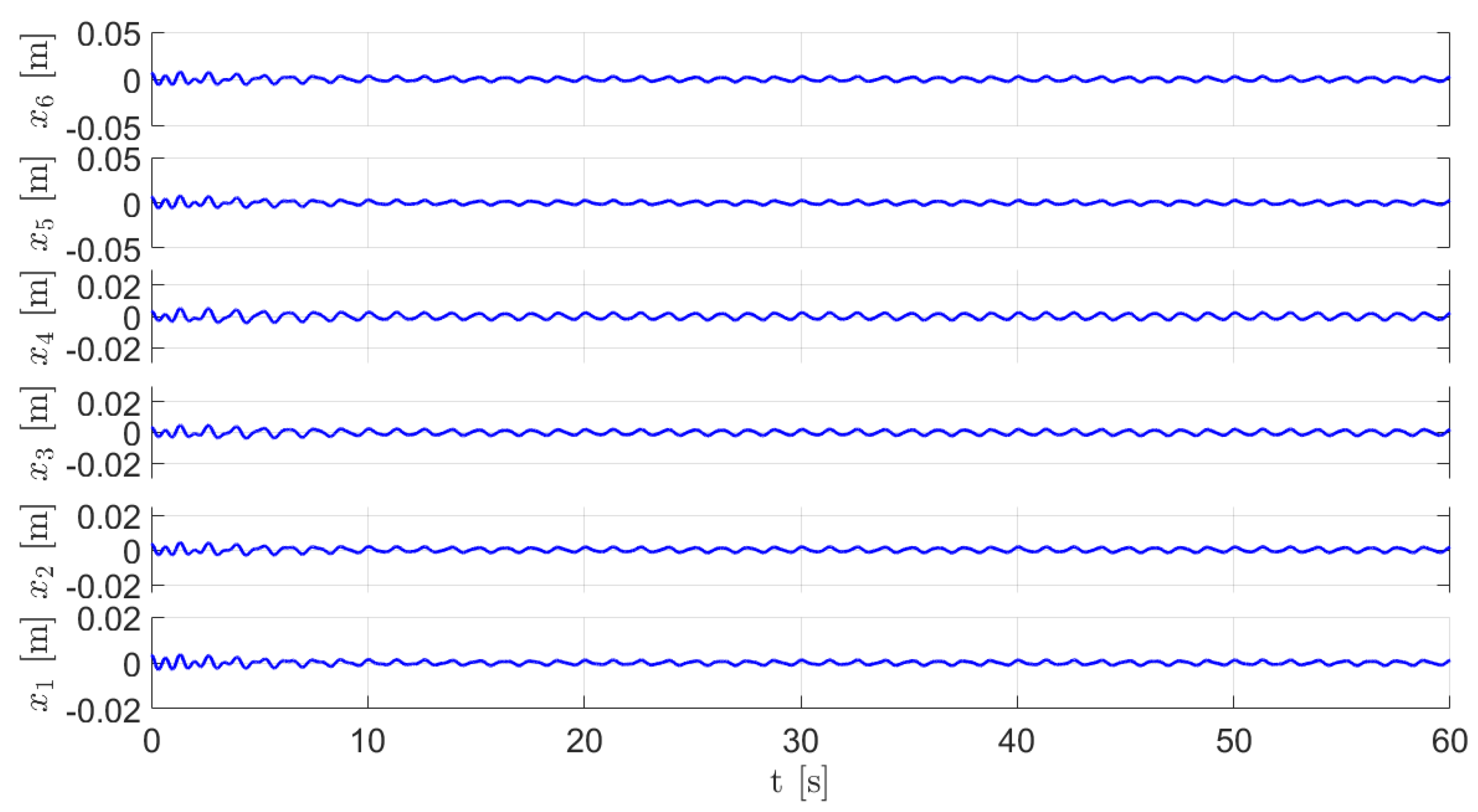
The dynamic behavior of the six-story building-like structure when the TMD-pendulum absorber is not tuned is described in Figure 6, where the amplitudes of vibration in stable state are $x_1\left(t\right)=10.58$ mm, $x_2\left(t\right)=15.85$ mm, $x_3\left(t\right)=20.61$ mm, $x_4\left(t\right)=23.86$ mm, $x_5\left(t\right)=25.28$ mm and $x_6\left(t\right)=27.18$ mm. Figure 7 shows the dynamic response of the flexible structure when experimentally (45) is satisfied. Now, the amplitudes of vibration in stable state are $x_1\left(t\right)=0.57$ mm, $x_2\left(t\right)=1.33$ mm, $x_3\left(t\right)=1.61$ mm, $x_4\left(t\right)=2.04$ mm, $x_5\left(t\right)=2.55$ mm and $x_6\left(t\right)=3.34$ mm, resulting in an average absorption percentage close to $91\%$.

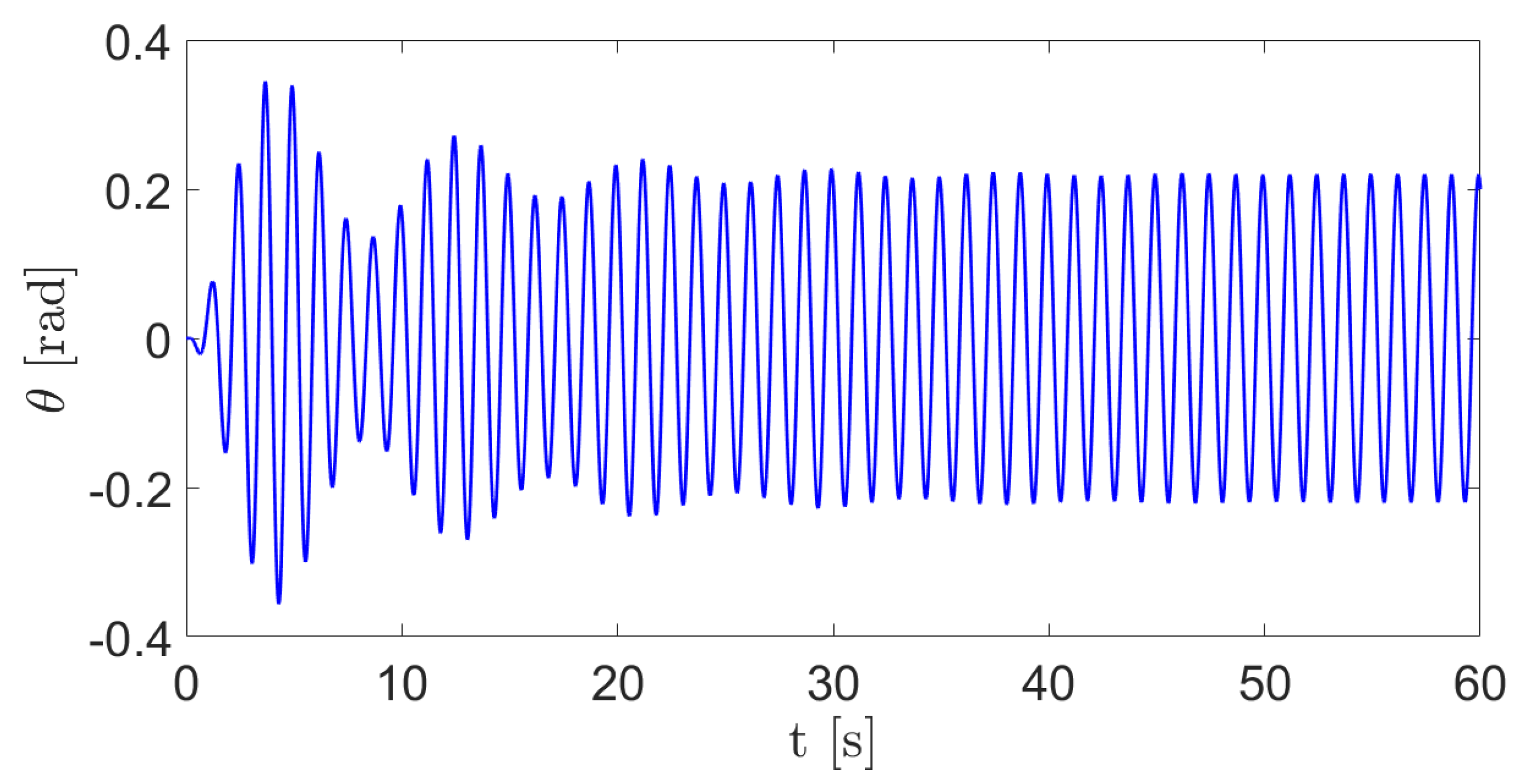
The linear absorber time history response, when the secondary system is tuned, is described in Figure 8. The stable state amplitude is $\theta \left(t\right)=0.22$ rad.

Figure 9 shows the performance of the on-line estimator (31) for the excitation force frequency. Acceptable estimations are obtained after $0.5$ s. The numerical value of the estimated frequency is $\widehat{{\Omega }}=1.069$ Hz.

5.3. Application of a Nonlinear Absorber

With the intention of showing that it is also possible to use the modal decomposition for the tuning of a nonlinear vibration absorber (independently of the number of degrees of freedom in the primary system), certain experiments were carried out with a pendulum type absorber, implemented in autoparametric form.

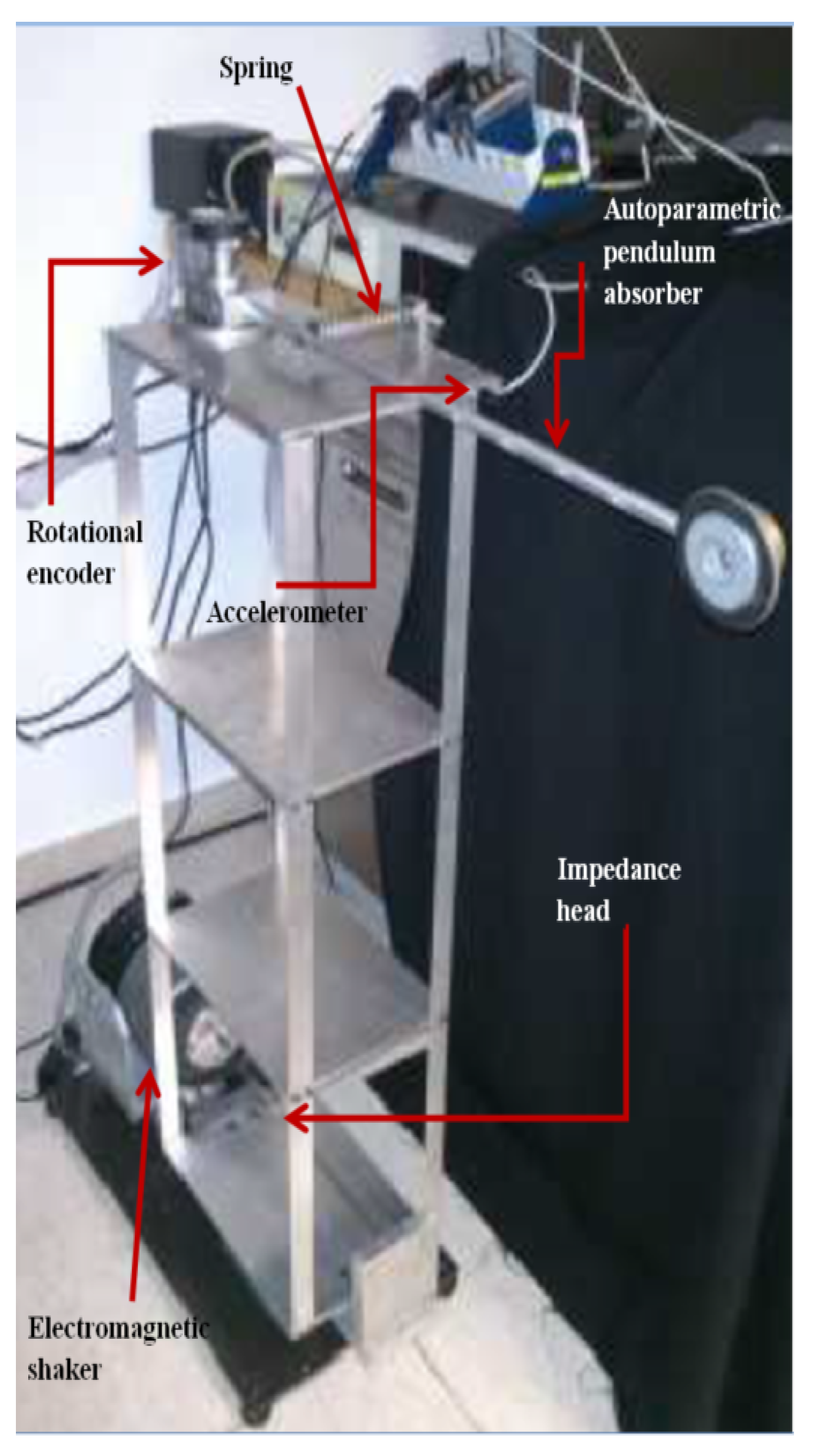
The experiment consisted in a flexible structure discretized in three degrees of freedom where a nonlinear vibration absorber (pendulum type) is coupled as shown in Figure 10. In this second case, we also use a high resolution rotational encoder to take angle measurements of the autoparametric pendulum absorber and a IEPE accelerometer, attached to the third story of the structure to take vibrations measurements. Once again, the electromechanical shaker acts as a source of excitation in conjunction with the frictionless slider. In this configuration, it is necessary to add a spring element in the secondary system in order to provide the pendulum with potential energy since its rotational dynamics occurs in a horizontal plane, so there are not gravity effects to be taken into account (see Figure 10). It results in the following nonlinear dynamic model

$$\begin{array}{ccc}\hfill M\ddot{x}+C\dot{x}+Kx+\varphi \left(\theta ,\dot{\theta },\ddot{\theta }\right)& =& B_{1}F\left(t\right)\hfill \end{array}$$

(46)

$$\begin{array}{ccc}\hfill m_a\ddot{\theta }+c_a\dot{\theta }+k_a\theta +\psi (\ddot{x},\theta )& =& 0\hfill \end{array}$$

(47)

where M, C and K are the $3\times 3$ matrices of mass, damping and stiffness. $B_1={\left[1,1,1\right]}^T$ is an input vector. Functions $\varphi \left(\theta ,\dot{\theta },\ddot{\theta }\right)$ and $\psi (\ddot{x},\theta )$ are defined as:

$$\varphi \left(\theta ,\dot{\theta },\ddot{\theta }\right)=\left[\begin{array}{c}0\\ 0\\ -m_{4}L(\ddot{\theta }\theta +{\dot{\theta }}^2)\end{array}\right],\psi (\ddot{x},\theta )=\left[-m_{4}L\theta {\ddot{x}}_3\right]$$

(48)

The parameter associated with the pendulum absorber is its equivalent mass $m_a=m_4{L}^2$, where L is the pendulum length.

It is evident that the nonlinear coupling between both subsystems is by means of $\varphi \left(\theta ,\dot{\theta },\ddot{\theta }\right)$ and $\psi (\ddot{x},\theta )$ which are defined by (48). These nonlinear functions allow the implementation of the autoparametric pendulum absorber in one specific vibration mode of the primary system.

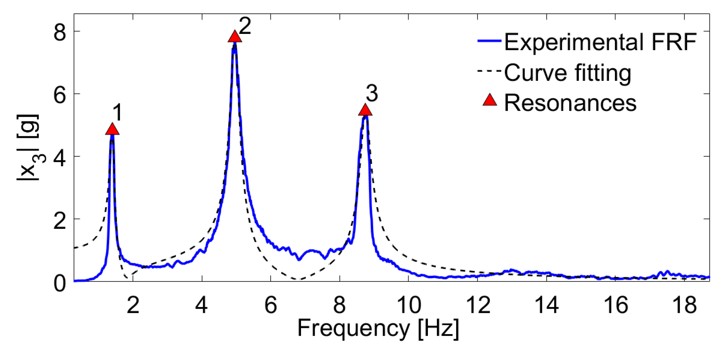
The frequency response function of the primary system with nonlinear pendulum absorber is described in Figure 11. In this type of nonlinear vibration systems, the frequency response function remains unchanged, i.e., no additional peaks are added in the aforementioned graph (which is a typical dynamic situation using a TMD absorber). Only the natural frequencies of the flexible structure change slightly in value due to the added mass (mass absorber).

5.4. Nonlinearity Analysis

Both primary systems analyzed in this work are assumed to be linear due to the nominal operating conditions considered, in addition to the characteristics of its construction material. Nevertheless, the vibration absorption scheme used to mitigate undesired effects of the first vibration mode of the structure is inherently non linear. 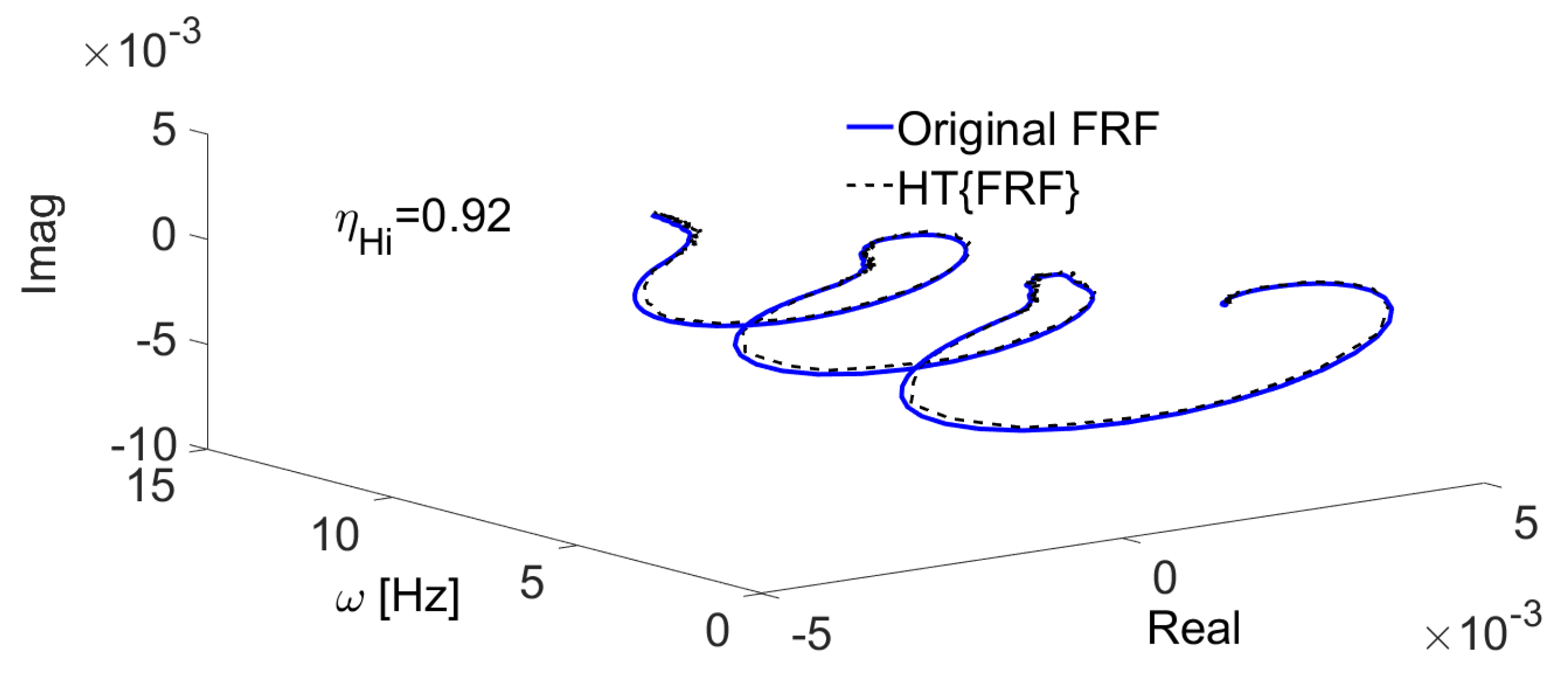In order to evaluate the influence of the nonlinear autoparametric pendulum absorber, we perform a nonlinearity analysis, using the nonlinearity index defined by (36), on the complete system (included the nonlinear vibrations absorber). The Nyquist diagram of the corresponding FRF of the system is shown in Figure 12 with its corresponding Hilbert transformation. The dashed black line, representing the Hilbert transformation of the FRF, does not show an important distortion.

The low distortion in the Nyquist diagram produced by the application of the Hilbert transformation suggests a linear behavior of the system in its nominal operational conditions. The nonlinearity index (35) of this particular building like structure including the nonlinear vibrations absorber is:

$${\eta }_{Hi}={∥R_{HG}\left(0\right)∥}^2=0.92$$

(49)

Thus, we can use the coefficients of the characteristic polynomial reported in

Table 3. Estimated coefficients of the characteristic polynomial.

Coefficient	Value
${\widehat{a}}_5$	4.6
${\widehat{a}}_4$	4417
${\widehat{a}}_3$	$1.4134\times {10}^4$
${\widehat{a}}_2$	$3.95435\times {10}^6$
${\widehat{a}}_1$	$6.64657\times {10}^6$
${\widehat{a}}_0$	$3.4632423\times {10}^8$

for the synthesis of an on-line algebraic identifier (31) for the harmonic excitation force.

The modal parameters obtained from experimental modal analysis by applying the curve fitting method for the case when a pendulum absorber (nonlinear-type) is applied are given in

Table 4. Modal parameters of the three-story building-like structure with nonlinear pendulum absorber.

Mode	Frequency [Hz]	Damping Ratio %
1	1.03	0.11
2	5.26	0.75
3	9.03	0.34

.

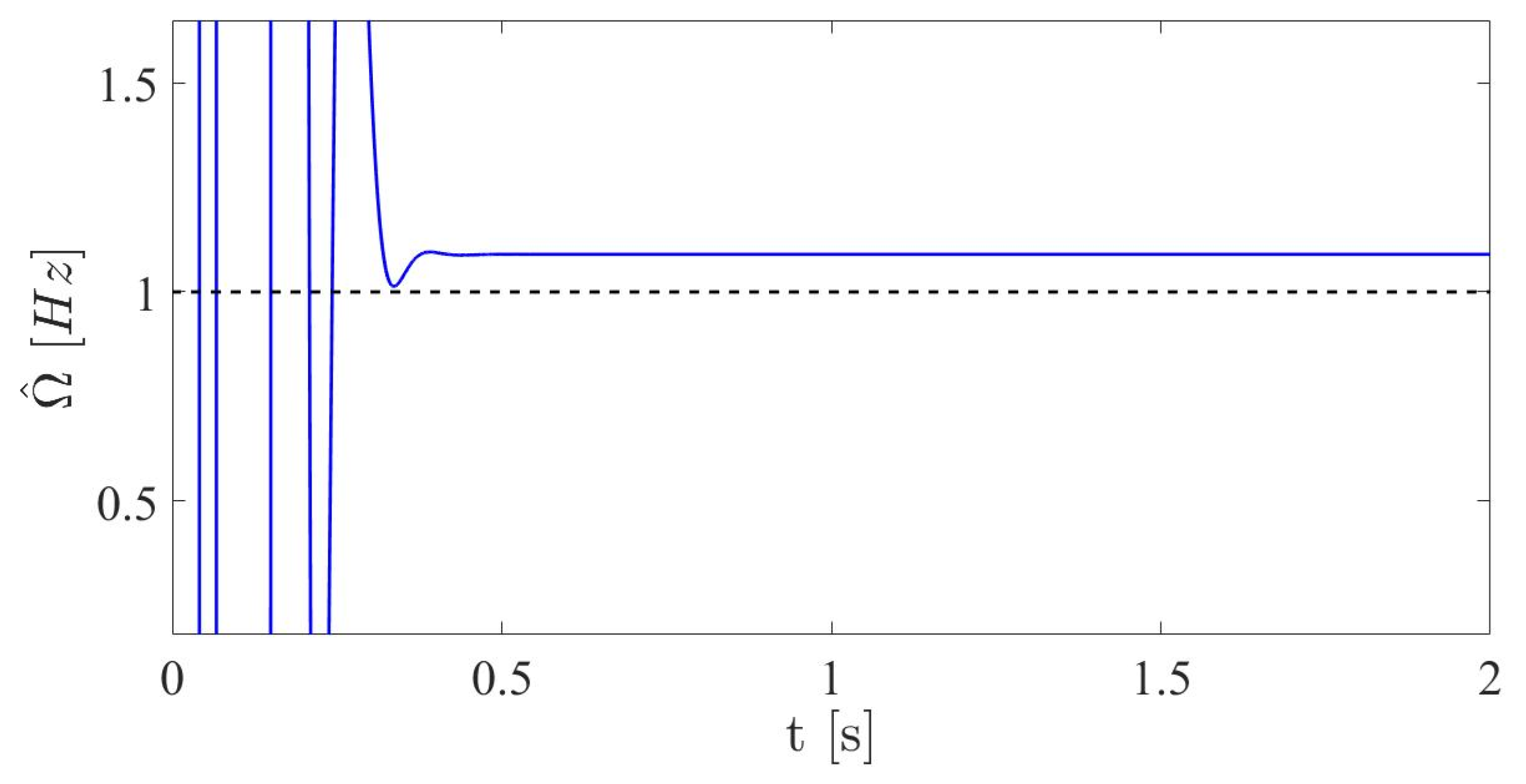
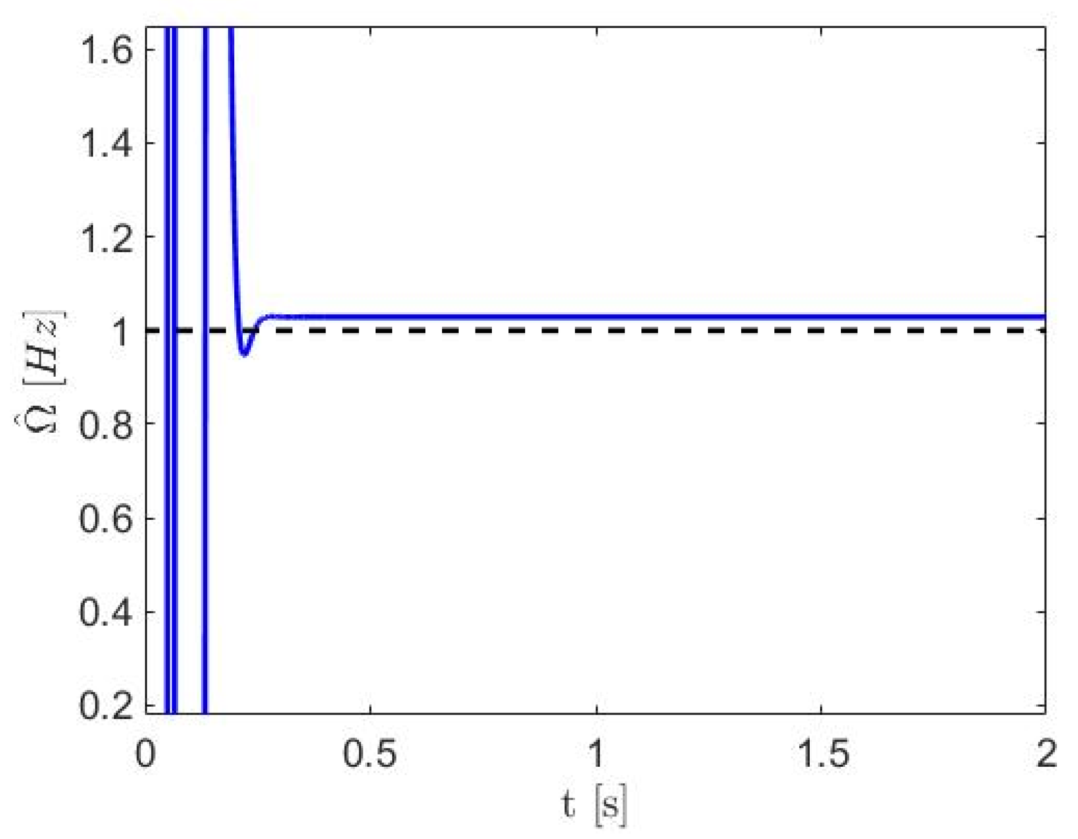
Coefficients of the characteristic polynomial are reported in Table 3. Those coefficients are used for the synthesis of an on-line algebraic identifier (30) for the harmonic excitation force. Figure 13 shows the performance of the on-line estimator (31) for the excitation frequency. Estimations are stable after only $0.5$ s. The numerical value for the on-line estimation parameter is ${\Omega }=1.039$ Hz after $0.48$ s.

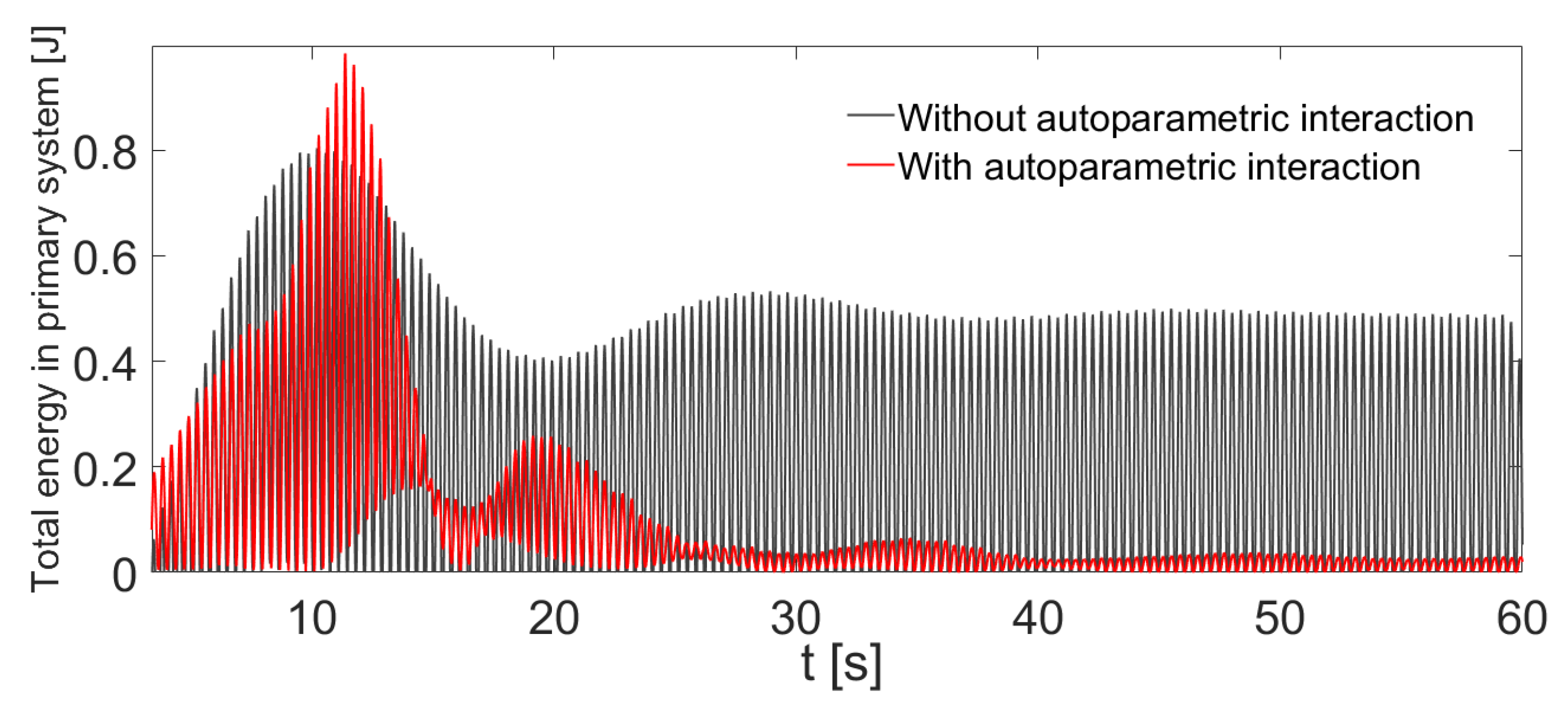
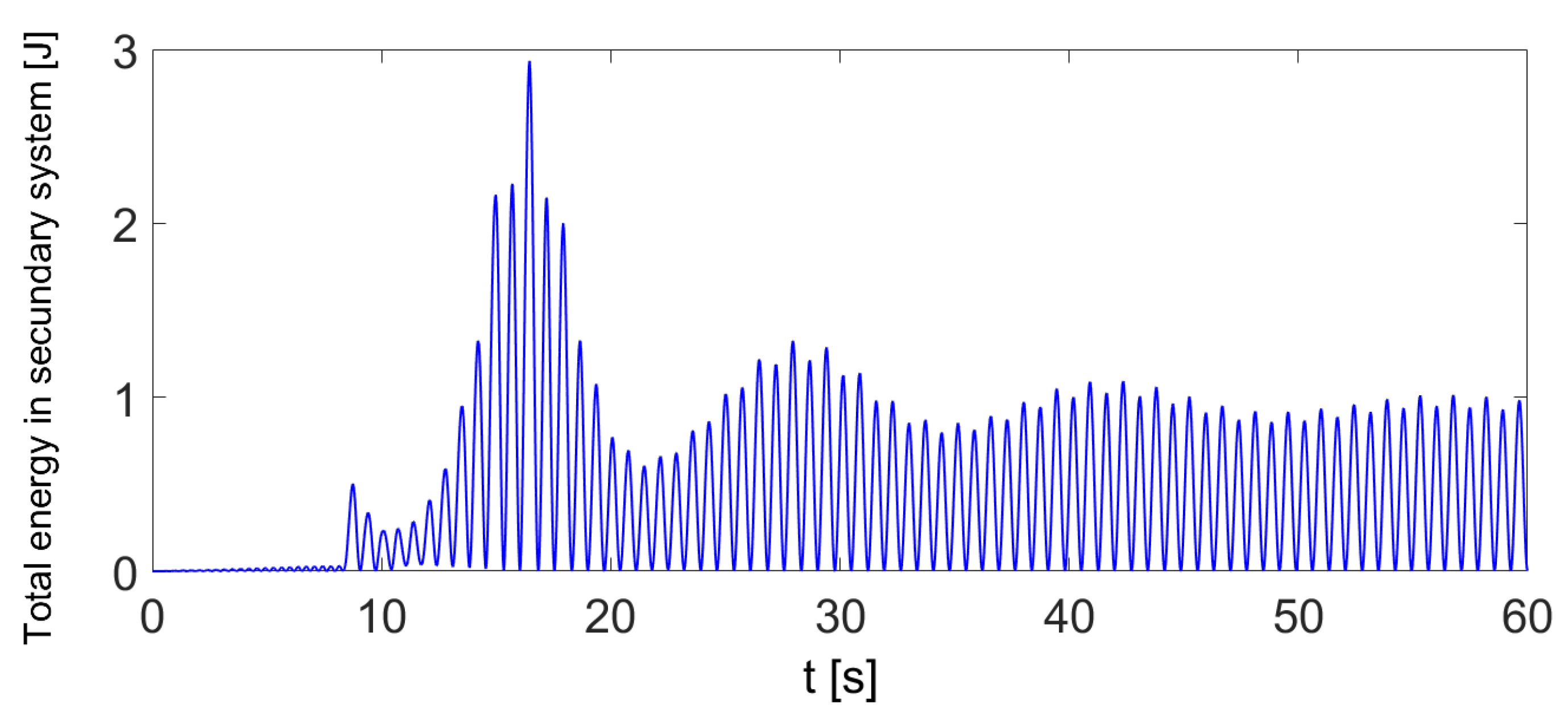
On the other hand, the dynamic performance in energy terms of the system shown in Figure 10, is described in Figure 14 and Figure 15, respectively. Once the transient response has disappeared the autoparametric absorber shows good dynamic performance dissipating a large percentage of the external energy supplied to the main structure.

6. Conclusions

In the present work, a comparison of a passive vibration control scheme applied to a flexible structure is studied experimentally. In order to mitigate resonant excitations, associated with the first mode of vibration, a pendulum absorber was implemented in two different configurations. It was observed that when the passive absorber was configured to work as an autoparametric system (nonlinear case), there were no significant changes in its frequency response function, this is because additional resonances are not introduced when this kind of dynamic vibration absorber is used, in contrast with the TMD configuration where this is a well known disadvantage.

Basically, the main advantage of an autoparametric vibration absorber is its property of high energy absorption exactly in resonant excitation. That is, when the external and internal resonance (autoresonance) conditions are tuned, the external energy affecting directly the main structure is transferred as kinetic energy (motion) to the autoparametric absorber and this situation results reasonable, because then the primary system can be protected from worst case dynamic conditions (resonance). It is important to mention that in both passive vibration absorbers, the effective damping should be small, otherwise the absorption capability would be significantly reduced. It is evident that there is a compromise about the amount of damping existing into the primary system and absorber, because stability and performance depend on this type of criteria. In general, small damping results in better vibration attenuation properties but at the same time makes the complete system more sensitive to endogenous perturbations. In addition, the performance of the on-line algebraic estimator for frequency of the excitation force showed a good efficiency using measurements of only one degree of freedom of the building-like structure, having the advantage of its estimation speed (it is achieved in less than a cycle of the original signal) in contrast with the fast-Fourier-transform (FFT)-based methods where at least one cycle of the signal is needed. Finally, the nonlinearity index tested here is easy to program and compute. In particular, we have assumed a value of ${\eta }_{Hi}\ge 0.9$ to establish that a given system is dominantly linear. Subsequent investigation on passive/active dynamic vibration absorption based on on-line algebraic identification of modal parameters and excitation forces on nonlinear multi-delay flexible structures will be considered in future work. Future research work will consider the implementation of multiple-frequency vibration absorption devices as well.