Abstract
This paper presents a new accurate multiple model of nonlinear pneumatic lateral forces. The bicycle representation is used in order to build up an easy implemented vehicle dynamic model. Moreover, the Takagi–Sugeno fuzzy approach is applied in order to handle the vehicle model nonlinearities. This structure allows for taking into account the small variation of the vehicle longitudinal velocity. Subsequently, a Fault Tolerant Control strategy that is based on a bank of fuzzy Luenberger observers is proposed. The robustness of the control scheme against external noises is guaranteed by applying performance. Sufficient stability conditions that are based on Lyapunov method are formulated as Linear Matrix Inequality. Thus, allowing the computation of the observers’ and the controllers’ gains by using MATLAB. Finally, the simulation examples are performed to show the effectiveness of our proposal.
1. Introduction
Recently, the automotive industrial companies have given more importance to the vehicle passengers security by introducing many active and passive safety systems. Because of the latest achievement in the field of embedded electronic systems, these solutions become more sophisticated, more reliable, less bulky, and less heavy [1]. These systems include Anti-lock Braking System (ABS), which allows for limiting the wheel lock during the braking phase, Dynamic Stability Control (DSC) and Electronic Stability Program (ESP) that are necessary to control the vehicle trajectory. The communication between these electronic systems is ensured by Controller Area Network (CAN) bus [2]. Thus, allowing for the Electronic Control Units (ECU) to share the information that is delivered by different sensors. Several researches in the literature have dealt with the vehicle Fault Tolerant Control (FTC) [3,4,5,6]. Generally, FTC strategies are classified into two categories. The first one deals only with a specified type of faults and uncertainties, and it is called Passive FTC (PFTC) or robust control [7,8]. While the second class also known as Active FTC (AFTC) requires a Fault Detection and Isolation (FDI) block [9,10]. When a fault occurs, it is detected and isolated using this online FDI. Subsequently, the controller is reconfigured [4,11]. Before establishing the FTC scheme, the first step consists in modelling the plant. The full vehicle model is very complex [12]. For this reason, a lot of attention has been paid to the simplified bicycle model [13,14]. Even though this model is simple, it is still nonlinear. The pneumatic lateral forces are the main origin of these nonlinearities. They are accurately modeled by the semiempirical Pacejka magic formula [15]. There are other physical models, such as the Brush tire model [16], the Dugoff, and the modified Dugoff formulas [17], but they are still less accurate.
In [18], a complete vehicle model has been developed to design FTC strategy for the yaw rate. In this study, the steering controller can operate normally, even in the occurrence of velocity controller faults. It is challenging to design a global control law directly from the nonlinear model [19]. Exciting new research shows that there is a different way to treat vehicle FTC [20,21,22]. It is very known that the control theory of linear system is well established. The idea is to find a convex interpolation of some linear systems that approximate correctly the nonlinear one. This is exactly the (T–S) fuzzy representation of the plant’s nonlinear behavior [23]. Then inspired from Lyapunov stability criterion applied to linear systems, one can design easily the observers and the controllers for the nonlinear model. In [16], a fuzzy robust control strategy of vehicle lateral dynamic is proposed while using sixteen linear submodels to take into account the small changes of longitudinal velocity. More recently, some researchers focus on the FTC strategies that tolerate to sensor and actuator faults while using the descriptor approach [24,25]. In the aforementioned works, there is no FTC strategy that simultaneously takes into account the slight variation of the vehicle longitudinal velocity, sensor faults, and the nonlinearity of the pneumatic forces. The later remark constitutes the first motivation for this research work. The main contributions of our paper are summarized in the following points:
- A simple and more accurate fuzzy representation of the lateral pneumatic forces as compared to the model adopted in [26,27]; the bell-shaped membership functions used in the fuzzy representation in [26,27] are not suitable.
- A multiple model of the vehicle lateral dynamic that takes into consideration the slight variation of the vehicle velocity at the design stage. Previous work such as [14,25] did not take this into account.
- The design of a less conservative FTC with noise rejection, which deals with sensor faults and eight multiple models
The conditions in terms of LMI are solved under MATLAB using YALMIP toolbox [28]. Thus, simultaneously guaranteeing the stability of the closed loop nonlinear system and its immunity to external disturbances.
Henceforth, in this work, the developed control strategy addresses both the combustion engine based vehicle and the Full Electric Vehicle (FEV). The technical details matter when implementing the algorithm in the microcontroller. By adopting a general paradigm, only mechanical features have a direct impact on the proposed methodology.
The subsequent parts of this paper are organized, as follows. Section 2 is dedicated to the multiple model representation of lateral forces. Section 3 proposes the T–S fuzzy model of the vehicle lateral dynamic. Section 4 describes the FTC strategy and the steps to obtain an LMI formulation that guarantees the optimization criterion. Section 5 presents simulation examples. Finally, Section 6 draws some conclusions and further perspectives.
2. Multiple Model of Pneumatic Lateral Forces
The linear model yields incorrect results due to the strong nonlinearity of the pneumatic lateral forces. The fuzzy paradigm can handle this issue. The first key step for establishing a multiple model of these pneumatic forces consists in modelling the vehicle lateral dynamic.
2.1. Modelling of the Vehicle Lateral Dynamic
Consider the classical bicycle model of a vehicle with a mass m and a yaw moment of inertia at the center of gravity as shown in Figure 1. This model was extensively used in the literature [29,30]. The following equations describe the vehicle lateral dynamics:
where , r, and denote respectively the sideslip angle, the yaw rate angle and longitudinal velocity. Front and rear tires lateral forces are represented by ,.While the parameters and designate, respectively, the distance between the rear axis, the front axis, and the vehicle center of gravity, as illustrated in Figure 1. The vehicle stability is controlled by the active yaw moment . In real applications, this external moment is generated by braking force allocation [31]. Firstly, the control torque needed in order to achieve the vehicle FTC strategy goal is calculated. Subsequetly, a microcontroller converts this information to individual wheel braking or all-wheel independent braking. This latest choice is based on the available technical solutions.
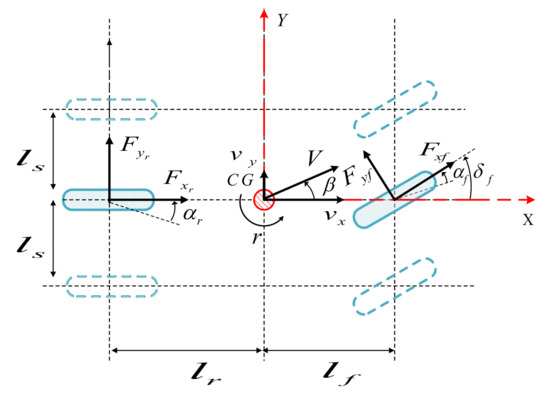
Figure 1.
The simplified vehicle lateral dynamics.
2.2. Multiple Model of Tire Lateral Forces
Let us consider that pneumatic lateral forces are described by the well-known Pacejka magic formulas, as given below [15]:
The coefficients , , , and , where x refers to r or f depend on several parameters, such as the road friction coefficient. The lateral forces change considerably when the corresponding tire slip angle () changes. Herein, our aim is to approximate equations in (3) by the following representation [26]:
where and are the weighting functions. In addition, , , , and are the coefficients of cornering stiffness of the front and rear tires. At this stage, one should discretize the reference curves of the lateral tire forces. This subsection deals only with the rear lateral force. In a similar way, the multiple model of the front tire lateral force can be determined.
In the literature, the bell curve membership functions are widely used. However, it does not give satisfactory results [27]. By the following, we define the new expression of the weighting functions:
The coefficients a and c verify:
It is noticed here that the system (4) is composed of three equations. While it contains six that are unknown. Therefore, the cornering coefficients are set in way to guarantee the convex sum property of the weighting functions [27]. Thus, the values of and are computed over the considered slip angle range. Figure 2 presents the weighting functions’ curves.
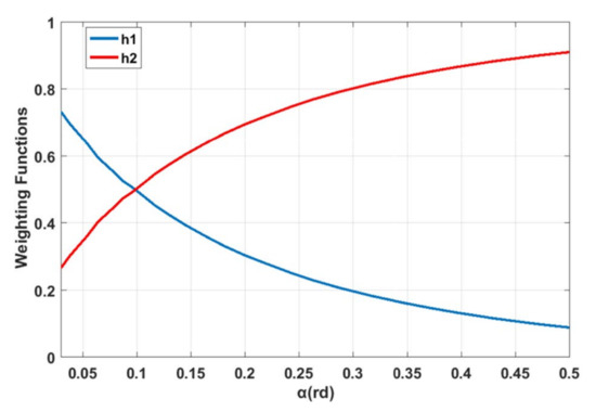
Figure 2.
and representative curves.
In order to compute the unknown parameters in (5), a MATLAB based curve-fitting algorithm is performed. Table 1 summarizes the results.

Table 1.
The values of lateral forces multiple model parameters.
Figure 3 depicts the comparison between three tire models. The linear one fails to pursue the evolution of the reference model. While the multiple model coincides considerably with the Pacejka model.
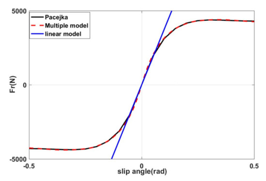
Figure 3.
Comparison of Pacejka model and the multiple model.
3. Vehicle T–S Fuzzy Model Formulation
The purpose of this section is to determinate the multiple model that accurately describes the nonlinear behavior of the vehicle lateral dynamics. The following equations are crucial in building the state space representation of the bicycle model [32]:
After replacing tire lateral forces by their expression in (4) and utilizing the formulas in (7), expressions (1) and (2) can be written, as follows:
where:
In this study, the variation of the vehicle longitudinal velocity during the steering is considered. Consequently, there is two nonlinearities in the state space model (8). The first function is , while the second is . By assuming that the vehicle velocity is bounded and, by applying the sector nonlinearity method [16], the following expression can be obtained:
where:
Subsequently, substituting (9) and (10) in (8) leads to the T–S fuzzy model of the vehicle lateral dynamics:
Matrices and and the membership functions are given in the Appendix A.
4. FTC of Vehicle T–S Fuzzy Model
When a sensor fault occurs in a critical situation, the vehicle lost its stability due to the faulty signal transmitted to the control unit. This may lead to dramatic consequences. For this reason, an observer based FTC strategy with a robust estimated state-feedback controller is proposed in this section. It is claimed that our system acquires two sensors. One to measure the sideslip angle while the other deals with the yaw rate. In addition, never all sensors fail at the same time.
4.1. Vehicle Closed Loop Fuzzy Model
Let us consider these two Fuzzy observers based on the classical Lunberger one:
where: , and with are the gains of the jth observer.
Because it is assumed in this study that the number of sensors is two. Accordingly, the same number of observer is needed (only for this case) to choose always the reconstructed state of the observer related to the healthy sensor. By taking advantage of the Parallel Distributed Compensation (PDC) technique, we define the following fuzzy feedback controllers:
Now, the jth error of estimation is defined as:
Gathering the Equations (11)–(16) leads to the following fuzzy augmented systems:
with and where:
4.2. Design of the Robust Fuzzy Controllers
In reality, the system environment may be a source of external perturbations; these disturbances directly affect the system performances. In order to increase the vehicle immunity against this type of issues, the constructed state feedback-controller is designed using the control approach. In this part, a more relaxed robust stability conditions are presented and formulated as LMI. It is worthy to note that the system that is considered here is the one in (17).
Definition 1.
the system (17) is considered stable with performance if it is stable and it verifies the following criterion:
where γ is a positive scalar that designates the attenuation. The following lemma is crucial in demonstrating the controller design procedure.
Lemma 1
([33,34]). let us consider a negative definite matrix Ξ. Given a full rank symmetric matrix Υ of appropriate dimension, then , such that:
Theorem 1.
the stability of the system (17) is guaranteed with the performance under the control of the kth feedback-controller if for a given , there exist symmetric positive matrices and and matrices , such that the following LMI is feasible:
with:
where:
with
Proof.
the first key step consists of choosing a Lyapunov function candidate. Therefore, let us consider the following quadratic one:
where is positive definite matrix, such as:
Now, the time derivative of the above Lyapunov function must be negative to ensure the stability of the given system. Deriving (22) yields:
Developing (24) leads to:
Criterion (18) is verified by ensuring the following inequality:
Substituting (23) in (24) yields:
where:
The inequality (26) is guaranteed if the following holds:
Using Schur complement [35], (28) and (29) are equivalent to:
with:
Developing the expression of leads us to:
with:
Now, we post and pre multiply by the following congruence matrix:
with:
The result can be expressed, as follows:
where:
Let us consider
By applying lemma 1, one can find:
In addition, these trivial inequalities holds:
The following inequality can be obtained:
where:
From (32) and (33) the following results can be deduced:
Using Schur complement, the following holds:
Since:
The LMI that figures in the proposed theorem gives sufficient and relaxed conditions that ensure the stability of the considered system with the performance. □
4.3. Description of the FTC Strategy
In order to improve the reliability and the availability of the vehicle lateral dynamics control system, it is mandatory to design a fault tolerant control scheme that maintains the normal functioning, even in the occurrence of sensor and actuator faults. In our study, we deal with sensor additive faults. The adopted FTC strategy is shown in Figure 4. Two observers estimate the vehicle state variable in real-time, each one uses the output of the corresponding sensor. There are two controllers that are connected to the observers. The previous theorem is used to compute the observers’ and the controllers’ gains in one-step. When a fault occurs, the residual signals in (36) are generated. Then, the decision bloc compares them with the predefined threshold. If one residual signal is greater than the switch receives the order to choose the controller related to the observer that uses the output of the healthy sensor.
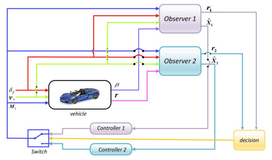
Figure 4.
Structure of the vehicle FTC Strategy.
5. Simulation Examples
In order to demonstrate the efficiency of the FTC strategy that was developed in this work and its capability to ensure a normal operation of the vehicle under sensor faults, we have proceeded by simulations that were performed in MATLAB/SIMULINK. Table 2 summarizes the vehicle parameters used in this section [36]. Figure 5 describes the longitudinal velocity profile. It is underlined here that all of the information needed to compute the state and control matrices of the T–S fuzzy model of the vehicle lateral dynamic are available.
Table 2.
The values of the vehicle parameters.
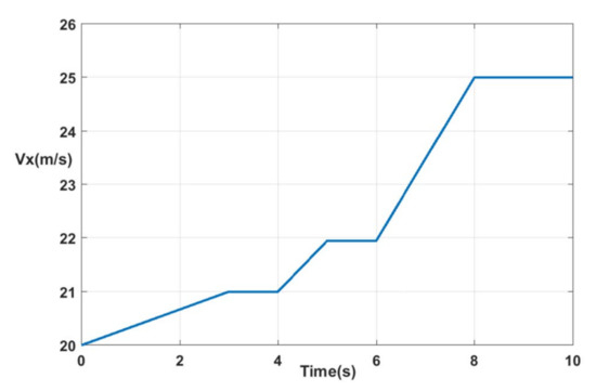
Figure 5.
Longitudinal velocity of the vehicle.
5.1. First Scenario
For the given profile of the front tire steering angle Figure 6 and the signal added to the measured yaw rate to represent the fault as described in Figure 7, we obtain the results that are shown below. Figure 8 and Figure 9 show the comparison between the vehicle sensors outputs and the estimated ones when the first observer, which is related to the faulty sensor, is used to control the vehicle lateral dynamics. It is noticed that the outputs do not follow the profile of the steering angle and reach high values when the fault occurs. In addition to that, the first observer fails to estimate the actual state vector. Accordingly, the vehicle directly loses its stability after the fault occurrence between 4 s and 10 s. Whereas, Figure 10 and Figure 11 expose, respectively, measured and estimated values of the yaw rate moment and the side slip angle after applying the above FTC strategy. It is remarked that the vehicle stability is guaranteed, even in the occurrence of the sensor fault. In addition, the figures show a good concordance between measured and estimated values over the predefined time range. Figure 12 exhibits the input control of the vehicle, which is the yaw moment. The switching from Controller 1 to Controller 2 is visualized clearly at 4 s (Figure 12). It is noticed that the switching is performed without a loss of system stability. From these figures, it is observed that the FTC strategy responds rapidly after the fault occurrence stabilizes the system by assigning the law control to the appropriate closed loop. The effect of the later action is seen directly by analyzing the results without FTC and those with FTC.
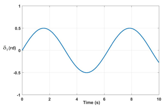
Figure 6.
Vehicle front steering angle.
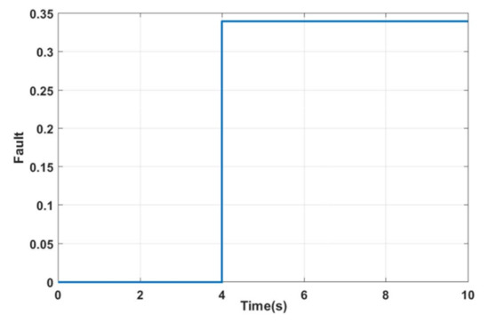
Figure 7.
Yaw rate sensor added signal.
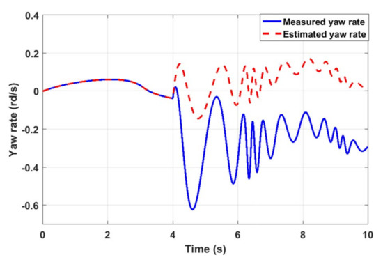
Figure 8.
Estimated vehicle Yaw rate without FTC Strategy.
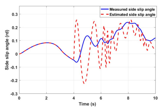
Figure 9.
Estimated vehicle sideslip angle without FTC Strategy.
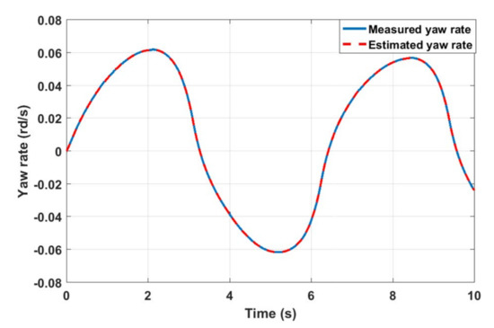
Figure 10.
Estimated vehicle Yaw rate with FTC Strategy.
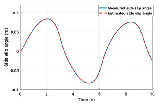
Figure 11.
Estimated vehicle sideslip with FTC Strategy.
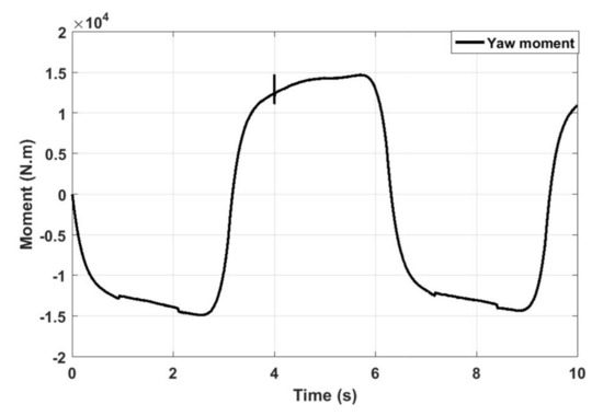
Figure 12.
Input control of the vehicle.
5.2. Second Scenario
In this subsection, we assess the system performances under the occurrence of successive faulty sensors. Based on the healthy sensor, the control strategy will recuperate the correct output signal. Figure 13 and Figure 14 show the signal profile of the added faults. The first one is added to the yaw rate sensor between 4 s and 6 s, while the second one is added to the measured side slip angle of the vehicle between 24.5 s and 30 s. In Figure 15, the switch effect is clear, and the effectiveness of the proposed FTC is demonstrated. A safe and normal operation of the vehicle is guaranteed between 0 s and 30 s.
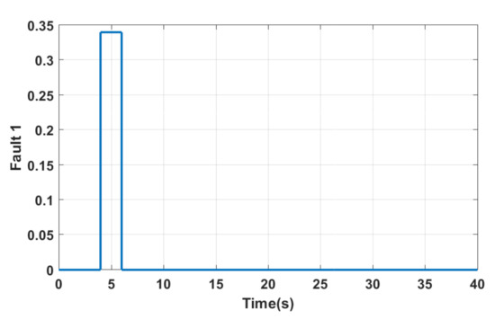
Figure 13.
Fault added to the yaw sensor.
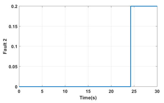
Figure 14.
Fault added to the output side slip angle.
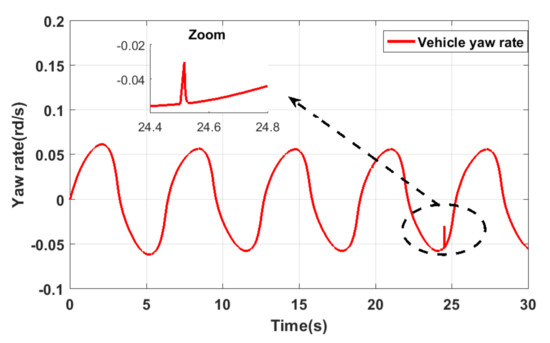
Figure 15.
Vehicle output Yaw rate with FTC.
5.3. Comparison
In order to show the added value of our method and its advantages when controlling a vehicle subjected to the longitudianl velocity variation and external disturbances, a comparison with the method proposed in [36] has been performed. In this simulation example, we adopted the steering angle profile described in Figure 16. The results that were obtained in Figure 17 show clearly the superiority of our method above the aforementioned technique. The difference observed in Figure 17 is due in particular to the use of filter, while the irregularities are caused by the variation of the vehicle speed, which is not taken into account when designing [36]. The results that were obtained by the proposed FTC strategy increase the immunity of the system against disturbances. Neglecting the system nonlinearity [37,38] or not modeling it precisely and the vehicle velocity variation when designing the FTC strategy leads to some divergence in the system outputs.
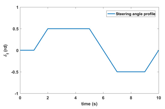
Figure 16.
Steering angle profile.
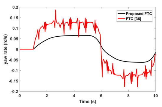
Figure 17.
Vehicle output Yaw rate comparison.
6. Conclusions
In this paper, a robust fault tolerant control methodology for vehicle lateral dynamics has been presented. We focused our efforts to establish the one presented in the second section due to the limitation of the lateral forces multiple or linear models available in the literature. This allows for us to build up the Fuzzy T–S multiple model of the vehicle lateral dynamics based on the well-known bicycle model. Subsequently, profiting from some results of the control theory we found out sufficient conditions to design a bank of observers on their correspondent controllers in terms of LMIs in one-step. Finally, simulation results are performed. The results show the importance of our approach. The main advantages of the proposed strategy are:
- The FTC designed in this work copes successfully with the nonlinear feature of the vehicle model.
- After the detection of a sensor fault, the stability of the system is guaranteed, even though the switching between controllers.
- performance ensures high immunity against noises and external disturbances.
Among the limits of the proposed FTC, it does not deal with the case of simultaneous sensor faults and the adopted vehicle model is not as accurate as the full vehicle model.
Future work may focuses on fault tolerant control of the vehicle while using more complex model to take into account the cross coupling between lateral and longitudinal velocities and including the model uncertainties.
Author Contributions
Conceptualization, I.A., M.N.K. and M.B.; methodology, I.A., M.N.K. and M.B.; software, I.A.; validation, I.A., M.N.K. and M.B.; writing the original draft, I.A.; writing the review version and editing, I.A., M.N.K. and M.B.; supervision, M.N.K. and M.B. All authors have read and agreed to the published version of the manuscript.
Funding
This research received no external funding.
Conflicts of Interest
The authors declare no conflict of interest.
Appendix A
The matrices and of T–S multiple model are as follows:
The membership functions are given as:
It is clear that the chosen membership functions satisfy the convex sum property.
Table A1.
Dimensions of matrices and vectors.
Table A1.
Dimensions of matrices and vectors.
| Matrices and Vectors | Dimension | Matrices and Vectors | Dimension |
|---|---|---|---|
| (2,2) | (2,1) | ||
| (2,1) | (2,2) | ||
| (2,1) | |||
| (2,2) | |||
| (1,2) | (1,2) | ||
| (2,1) | (1,2) | ||
| (4,4) | (4,1) | ||
| (2,2) | (2,2) | ||
| (2,2) | (2,4) | ||
| (2,1) | (1,2) | ||
| (12,12) | (2,2) | ||
| (2,2) | (4,4) | ||
| (2,2) | (5,1) | ||
| (5,5) | (7,7) | ||
| (7,7) | (2,2) | ||
| (2,2) | (2,1) | ||
| (2,1) | (2,1) | ||
| (2,1) | (4,1) | ||
| (5,5) | (2,2) | ||
| (2,2) | (2,2) |
References
- Gananchchelvi, P.; Jiao, Y.; Pukish, M.S. Current trends in in-vehicle electrical engineering applications. In Proceedings of the IECON 2012 38th Annual Conference on IEEE Industrial Electronics Society, Montreal, QC, Canada, 25–28 October 2012; pp. 6268–6273. [Google Scholar] [CrossRef]
- Guo, S. The application of CAN-bus technology in the vehicle. In Proceedings of the 2011 International Conference on Mechatronic Science, Electric Engineering and Computer (MEC), Jilin, China, 19–22 August 2011; pp. 755–758. [Google Scholar] [CrossRef]
- Oudghiri-Bentaie, M.; Chadli, M. Control and Sensor Fault-Tolerance of Vehicle Lateral Dynamics. FAC Proc. Vol. 2008, 41, 123–128. [Google Scholar]
- El Youssfi, N.; Oudghiri, M.; Bachtiri, E.R. Control design and sensors fault tolerant for vehicle dynamics (a selected paper from SSD’17). Int. J. Digit. Signals Smart Syst. 2018, 1, 50–67. [Google Scholar] [CrossRef]
- Luo, Y.; Hu, Y.; Jiang, F.; Chen, R.; Wang, Y. Active Fault-Tolerant Control Based on Multiple Input Multiple Output-Model Free Adaptive Control for Four Wheel Independently Driven Electric Vehicle Drive System. Appl. Sci. 2019, 9, 276. [Google Scholar] [CrossRef]
- Sun, J.; Cong, J.; Gu, L.; Dong, M. Fault-tolerant control for vehicle with vertical and lateral dynamics. Proc. Inst. Mech. Eng. Part D 2019, 233, 3165–3184. [Google Scholar] [CrossRef]
- Du, H.; Zhang, N.; Dong, G. Stabilizing Vehicle Lateral Dynamics With Considerations of Parameter Uncertainties and Control Saturation Through Robust Yaw Control. IEEE Trans. Veh. Technol. 2010, 59, 2593–2597. [Google Scholar] [CrossRef]
- Abzi, I.; Kabbaj, M.; Benbrahim, M. Design of Fractional Order Sliding Mode Controller for Lateral Dynamics of Electric Vehicles. In Proceedings of the 2nd International Conference on Electronic Engineering and Renewable Energy Systems, ICEERE 2020, Saidia, Morocco, 13–15 April 2020; Springer: Singapore; Volume 681, pp. 573–581. [Google Scholar]
- Alaridh, I.; Aitouche, A.; Zemouche, A. Chapter 10—Actuator and Sensor Fault Detection Based on LPV Unknown Input Observer Applied to Lateral Vehicle Dynamics. In New Trends in Observer-Based Control; Boubaker, O., Zhu, Q., Mahmoud, M.S., Ragot, J., Karimi, H.R., Dávilla, J., Eds.; Emerging Methodologies and Applications in Modelling; Academic Press: Cambridge, MA, USA, 2019; pp. 267–287. [Google Scholar] [CrossRef]
- Huang, C.; Naghdy, F.; Du, H. FDI Based Fault-Tolerant Control for Steer-by-Wire Systems. In Proceedings of the 2018 IEEE Conference on Control Technology and Applications (CCTA), Copenhagen, Denmark, 21–24 August 2018; pp. 199–204. [Google Scholar]
- Wang, D.; Li, Y. Fault tolerant control with actuation reconfiguration. In Proceedings of the Fifth World Congress on Intelligent Control and Automation (IEEE Cat. No.04EX788), Hangzhou, China, 15–19 June 2004; Volume 2, pp. 1506–1509. [Google Scholar]
- Parra, A.; Cagigas, D.; Zubizarreta, A.; Rodríguez, A.J.; Prieto, P. Modelling and Validation of Full Vehicle Model based on a Novel Multibody Formulation. In Proceedings of the IECON 2019 45th Annual Conference of the IEEE Industrial Electronics Society, Lisbon, Portugal, 14–17 October 2019; Volume 1, pp. 675–680. [Google Scholar]
- Aouaouda, S.; Chadli, M.; Bouhali, O. Observer-based fault tolerant tracking control for vehicule lateral dynamics. In Proceedings of the 2013 International Conference on Control, Decision and Information Technologies (CoDIT), Hammamet, Tunisia, 6–8 May 2013; pp. 51–56. [Google Scholar] [CrossRef]
- Coskun, S.; gari, R. Improved Vehicle Lateral Dynamics with Takagi–Sugeno H∞, Fuzzy Control Strategy for Emergency Maneuvering. In Proceedings of the 2018 IEEE Conference on Control Technology and Applications (CCTA), Copenhagen, Denmark, 21–24 August 2018; pp. 859–864. [Google Scholar] [CrossRef]
- Bakker, E.; Pacejka, H.B.; Lidner, L. A New Tire Model with an Application in Vehicle Dynamics Studies; SAE Technical Paper; SAE International: Monte Carlo, Monaco, 1989. [Google Scholar] [CrossRef]
- Jin, X.; Yu, Z.; Yin, G.; Wang, J. Improving Vehicle Handling Stability Based on Combined AFS and DYC System via Robust Takagi–Sugeno Fuzzy Control. IEEE Trans. Intell. Transp. Syst. 2018, 19, 2696–2707. [Google Scholar] [CrossRef]
- Bhoraskar, A.; Sakthivel, P. A review and a comparison of Dugoff and modified Dugoff formula with Magic formula. In Proceedings of the 2017 International Conference on Nascent Technologies in Engineering (ICNTE), Navi Mumbai, India, 27–28 January 2017; pp. 1–4. [Google Scholar] [CrossRef]
- Hernández-Alcantara, D.; Amezquita-Brooks, L.; Morales-Menéndez, R.; Olivier Sename, R. The cross-coupling of lateral-longitudinal vehicle dynamics: Towards decentralized Fault-Tolerant Control Schemes. Mechatronics 2018, 50, 377–393. [Google Scholar] [CrossRef]
- Petrov, P.; Nashashibi, F. Modeling and Nonlinear Adaptive Control for Autonomous Vehicle Overtaking. IEEE Trans. Intell. Transp. Syst. 2014, 15, 1643–1656. [Google Scholar] [CrossRef]
- Aouaouda, S.; Chadli, M.; Righi, I. Active FTC Approach Design for T–S Fuzzy Systems Under Actuator Saturation. In Proceedings of the 2019 6th International Conference on Control, Decision and Information Technologies (CoDIT), Paris, France, 23–26 April 2019; pp. 483–488. [Google Scholar]
- You, F.; Li, M. Fault tolerant control for T–S fuzzy systems with interval time-varying delay. In Proceedings of the 2017 Chinese Automation Congress (CAC), Jinan, China, 20–22 October 2017; pp. 223–228. [Google Scholar]
- Lan, J.; Patton, R.J. Integrated Design of Fault-Tolerant Control for Nonlinear Systems Based on Fault Estimation and T–S Fuzzy Modeling. IEEE Trans. Fuzzy Syst. 2017, 25, 1141–1154. [Google Scholar] [CrossRef]
- Takagi, T.; Sugeno, M. Fuzzy identification of systems and its applications to modeling and control. IEEE Trans. Syst. Man Cybern. 1985, SMC-15, 116–132. [Google Scholar] [CrossRef]
- Dhouha, K.; Hamdi, G.; El hajjaji, A.; Chaabane, M. Adaptive Observer and Fault Tolerant Control for Takagi–Sugeno Descriptor Nonlinear Systems with Sensor and Actuator Faults. Int. J. Control. Autom. Syst. 2018, 16, 972–982. [Google Scholar] [CrossRef]
- Aouaouda, S.; Chadli, M.; Boukhnifer, M.; Karimi, H.R. Robust fault tolerant tracking controller design for vehicle dynamics: A descriptor approach. Mechatronics 2015, 30, 316–326. [Google Scholar] [CrossRef]
- Dahmani, H.; Pagès, O.; El Hajjaji, A.; Daraoui, N. Observer-Based Robust Control of Vehicle Dynamics for Rollover Mitigation in Critical Situations. IEEE Trans. Intell. Transp. Syst. 2014, 15, 274–284. [Google Scholar] [CrossRef]
- Oudghiri, M. Commande Multi Modèles Tolérante aux Défauts: Application au Contrôle de la Dynamique d’un Véhicule Automobile. Ph.D. Thesis, Université de Picardie Jules Verne, Amiens, France, 2008. [Google Scholar]
- Kharrat, D.; Gassara, H.; El-hajjaji, A.; Chaabane, M. Delay-Partitioning Approach to State and Sensor/Actuator Fault Estimation for T–S Fuzzy Systems with Time-Delay. In Proceedings of the 2018 IEEE International Conference on Fuzzy Systems (FUZZ-IEEE), Rio de Janeiro, Brazil, 8–13 July 2018; pp. 1–7. [Google Scholar] [CrossRef]
- Polack, P.; Altché, F.; d’Andréa-Novel, B.; de La Fortelle, A. The kinematic bicycle model: A consistent model for planning feasible trajectories for autonomous vehicles? In Proceedings of the 2017 IEEE Intelligent Vehicles Symposium (IV), Los Angeles, CA, USA, 11–14 June 2017; pp. 812–818. [Google Scholar]
- Zhang, H.; Wang, J. Vehicle Lateral Dynamics Control Through AFS/DYC and Robust Gain-Scheduling Approach. IEEE Trans. Veh. Technol. 2016, 65, 489–494. [Google Scholar] [CrossRef]
- Zhang, L.; Yu, L.; Wang, Z.; Zuo, L.; Song, J. All-Wheel Braking Force Allocation During a Braking-in-Turn Maneuver for Vehicles With the Brake-by-Wire System Considering Braking Efficiency and Stability. IEEE Trans. Veh. Technol. 2016, 65, 4752–4767. [Google Scholar] [CrossRef]
- Guo, H.; Liu, F.; Xu, F.; Chen, H.; Cao, D.; Ji, Y. Nonlinear Model Predictive Lateral Stability Control of Active Chassis for Intelligent Vehicles and Its FPGA Implementation. IEEE Trans. Syst. Man Cybern. Syst. 2019, 49, 2–13. [Google Scholar] [CrossRef]
- Guerra, T.; Kruszewski, A.; Vermeiren, L.; Tirmant, H. Conditions of output stabilization for nonlinear models in the Takagi–Sugeno’s form. Fuzzy Sets Syst. 2006, 157, 1248–1259. [Google Scholar] [CrossRef]
- Kharrat, D.; Gassara, H.; Chaabane, M.; El-Hajjaji, A. Fault tolerant control based on adaptive observer for Takagi–Sugeno fuzzy descriptor systems. In Proceedings of the 2015 16th International Conference on Sciences and Techniques of Automatic Control and Computer Engineering (STA), Monastir, Tunisia, 21–23 December 2015; pp. 273–278. [Google Scholar] [CrossRef]
- Boyd, S.; Ghaoui, L.; Feron, E.; Balakrishnan, V. Linear Matrix Inequalities in System and Control Theory; SIAM: Philadelphia, PA, USA, 1994. [Google Scholar]
- Oudghiri, M.; Chadli, M.; Hajjaji, A. Robust Observer-based Fault-tolerant Control for Vehicle Lateral Dynamics. Int. J. Veh. Des. 2008, 48, 173–189. [Google Scholar] [CrossRef]
- Takagi, T.; Sugeno, M. Robust output-feedback yaw control for in-wheel motor driven electric vehicles with differential steering. Neurocomputing 2016, 173, 676–684. [Google Scholar] [CrossRef]
- Ding, S.X.; Schneider, S.; Ding, E.L.; Rehm, A. Fault tolerant monitoring of vehicle lateral dynamics stabilization systems. In Proceedings of the 44th IEEE Conference on Decision and Control, Seville, Spain, 15 December 2005; pp. 2000–2005. [Google Scholar] [CrossRef]
Publisher’s Note: MDPI stays neutral with regard to jurisdictional claims in published maps and institutional affiliations. |
© 2020 by the authors. Licensee MDPI, Basel, Switzerland. This article is an open access article distributed under the terms and conditions of the Creative Commons Attribution (CC BY) license (http://creativecommons.org/licenses/by/4.0/).