On-Line Open-Phase Fault Detection Method for Switched Reluctance Motors with Bus Current Measurement

Abstract

This article introduces an on-line fault diagnosis (FD) system to detect and recognize open-phase faults in switched reluctance motors (SRMs). Both tasks, detection and recognition, are based on functions built with the same information but from different sources. Specifically, these functions are constructed from bus current measurement provided by a sensor and from the estimate of such a current provided by an extended Kalman filter (EKF) that performs the estimation from only rotor angular position measurements. In short, the FD system only requires two measurements for employment: bus current and angular position. In order to show its efficacy, results from numerical simulations (performed in a virtual test bench) are presented. Specifically, these simulations involve the dynamics of the SRM, including the magnetic phenomena caused by the analyzed faults. The motor dynamics were obtained with finite element simulations, which guarantee results close to the actual ones.

1. Introduction

The switched reluctance motor (SRM) is characterized by its low cost, efficiency and robust structure. On the one hand, this motor has windings concentrated in the stator; therefore, the phases are magnetically and electrically independent. On the other hand, the rotor is made only of laminated steel, so it has a low shaft inertia that allows the motor to respond quickly to sudden changes in acceleration. These characteristics have made the SRM an interesting candidate for wind turbines and electric vehicles’ design, as shown in [1,2,3].

As with all industrial processes, however, SRM-based systems are subjected to undesirable stresses, which could cause some faults to become failures. For this reason, researchers have devoted a lot of effort studying a variety of motor faults, such as winding and bearing faults, unbalanced stators, unbalanced rotors, broken rotor bars and eccentricity [4]. Of all these faults, those in the stator represent approximately $30\%$ to $40\%$ of the total because the stator is constantly subject to thermal, electrical, mechanical and environmental stresses [4,5]. In addition, there are no electrical faults in the rotor since only the stator has windings.

According to [6], electrical stator-phase faults can be classified as follows: inter-turn short-circuits of a coil, inter-phase short-circuits, one coil short-circuit in a phase winding, an open circuit of a coil, short-circuits of the coils and an open circuit of the whole winding, which is equivalent to a lost phase. The works by [7,8] suggest that the most common and critical fault in the stator windings of the SRM is open circuit winding, i.e., open-phase fault.

Several examples of fast Fourier transform (FFT)-based methods can be found in the fault detection literature. For example, the work by [9], where short-circuit faults are diagnosed through an FFT method where the peak current value in the frequency response is used to detect the fault. The paper by [10] also uses the FFT method to determine symmetrical components to construct a fault index ratio that is employed to detect short-circuit faults. The work by [11] proposes an FFT-based method using only the bus current signal. This method detects harmonics that appear in the bus current spectrum after a fault. By normalizing the harmonics amplitude, a fault signature is obtained.

Other types of fault detection methods are the model-based ones. These methods are mainly funded on state estimators, such as the Kalman filter. Most of these fault detection methods have been designed for other types of motors or motor drives. For example, the work by [12] presents an off-line method that diagnoses an open-phase fault when the stator resistance, estimated using an extended Kalman filter (EKF), exceeds its nominal value. The paper by [13] proposes the estimation of phase currents using an EKF for detection of open-phase faults. It is worth noting that in this case the EKF inputs are the measured currents; therefore, the estimated current may be affected by the phase current fault. The detection is achieved by evaluating the difference between the phase current measurements and their estimates. In [14] the inter-turn faults are detected using an EKF and total harmonic distortion. While in [15], the short-circuit fault diagnostics are also made using an EKF. In particular, two examples of diagnosis methods based on the EKF for the SRM, are as follows: ref [16], in which winding resistance is estimated to help detect inter-turn faults, and [17], in which the inter-turn fault is detected from chopping switching signals. A recent survey on detection and isolation methods for the SRM was presented in [18]. It mentions that Kalman filter-based methods have the disadvantage of long calculation times. Nevertheless, these methods have high robustness and low cost.

In this spirit, the goal of this paper was the introduction of an on-line method for detecting and recognizing (identifying) open-phase faults using only measured bus current. The proposed method is based on analytical relations (ARs), which are functions constructed from measured bus current and its estimate, i.e., from the same information but from different sources. The estimate of the bus current is generated by an EKF that involves an actualization term that depends on a measured angular position. The detection and recognition of the fault are made on-line by comparing the ARs with a threshold.

It must be mentioned that in [19], it is presented a first attempt to solve this problem using an EKF. The main differences between that conference article and the proposed method in this paper are:

• In [19], the EKF uses the four stator current measurements. On the contrary, the fault diagnosis (FD) system proposed in this article only needs the bus current knowledge.
• The signature matrix in the conference paper is different. In that article, the Flag is activated when the residual is negative. On the contrary, the FD system proposed in this article requires to define a positive threshold for the fault detection.
• In the conference paper only a one-phase fault is studied. Conversely, The FD system proposed can detect when two phases are in fault.
• This contribution presents a validation by using signals obtained from a more realistic motor model which is based on the Maxwell’s equations that are solved with FEM.
• This paper presents a comparison between our proposed FD method and a widely used FFT method.
• The FD system proposed in this article includes an optimization stage for identifying the faulty phases when two faulty phases are present.

In order to evaluate the efficacy and suitability of the proposed fault detection (FD) system, a virtual test bench (VTB) was developed. The VTB used in this contribution is integrated by a finite element (FE) model of the SRM implemented in Altair Flux together with a controller and the FD system implemented in MATLAB Simulink. FE models are used to study systems under faulty conditions as in [20,21] or to verify proposed thermal models as in [22]. Finite element models have been shown to be useful in giving insight into the behavior of real systems, as demonstrated in [23].

The advantages of the proposed method are seen bellow:

• It is an on-line method.
• The proposed method uses only information from the measured bus current, the angular position, number of stator phases and number of rotor poles.
• The FD system does not need to store data to obtain a diagnostic.
• The proposed method is robust because stator currents are reconstructed using only measured angular position. This means the fault will not affect the AR calculation.

The main disadvantage of the proposed method is that it is only valid for low speeds below the SRM base speed.

This paper is organized as follows. Section 2 provides preliminaries: the mathematical model of SRM, observability analysis and controller equations. Section 3 presents the main result: EKF implementation, fault detection and identification method. Section 4 is devoted to a numerical system model based on co-simulation, and Section 5 is dedicated to the evaluation and comparison of the fault detection and recognition method. Finally, Section 7 draws the conclusions of the article.

2. Preliminaries

This section presents the mathematical model of the SRM, an observability analysis based on this model, as well as the model-based controller used in this article. The observability analysis is important because it is used for conceiving the observer-based FD method proposed.

2.1. Switched Reluctance Motor Features

The SRM has salient poles in both the stator and rotor, where the number of stator poles is $N_s$, while the number of rotor poles is $N_r$. The regular SRM complies with $N_r=N_s\pm 2$ to provide continuous unidirectional torque, with the ability to ensure starting torque from any rotor position: there are no zero-torque positions [24]. For example, Figure 1 presents a four-phase 8/6 SRM; therefore, for this motor $N_r=N_s-2$. This machine can produce torque over an arc of rotation, when the overlap angle between the rotor and stator poles is varying. For example, positive motoring torque is produced while inductance is increasing as the rotor approaches the aligned position. Therefore, the stator phases must be sequentially switched to attract the rotor poles to generate continuous movement of the rotor shaft.

Simultaneously, the windings in this type of machine may be connected either in series or in parallel [25]. In this respect, it is important to mention that the result presented here is only valid for windings in parallel connection. As mentioned by [26] continuous operation of the SRM is only possible after an open-phase fault has occurred in this type of SRM.

For this machine, the standard assumptions for a first-harmonic mathematical model [27] are the following:

A.1

Mutual inductances are negligible: stator phases are electrically and magnetically independent.

A.2

Winding inductance is defined as

$$\begin{array}{cc}\hfill L_{\mathit{j}}\left(\theta \right)& =l_0-l_{1}cos\left(N_r\theta \left(t\right)-(\mathit{j}-1)\frac{2\pi }{m}\right),\hfill \end{array}$$

(1)

where $j=1,2,3,\dots ,m$ is the phase index, with m as the number of stator phases. Moreover, $\theta \in \mathbb{R}$ is the angular rotor position, and $l_0>l_1>0$ are the inductance coefficients.

A.3

Stator flux linkage ${\lambda }_{\mathit{j}}$ is defined as

$$\begin{array}{c}\hfill {\lambda }_j=L_{\mathit{j}}\left(\theta \right)i_j\left(t\right),\end{array}$$

(2)

where $i_{\mathit{j}}$ is stator phase current, with $i_j$ lower than the saturation current [28].

Therefore, the mathematical model of the SRM is given by:

$$\begin{array}{cc}\hfill \frac{d\mathit{i}\left(t\right)}{dt}& ={\mathbf{L}}^{-1}\left(\theta \right)\left(\mathit{u}\left(t\right)-\omega \left(t\right)\mathbf{C}\left(\theta \right)\mathit{i}\left(t\right)-\mathbf{R}\mathit{i}\left(t\right)\right)\hfill \end{array}$$

(3a)

$$\begin{array}{cc}\hfill \dot{\theta }\left(t\right)& =\omega \left(t\right)\hfill \end{array}$$

(3b)

$$\begin{array}{cc}\hfill \dot{\omega }\left(t\right)& =\frac{1}{\mathrm{J}}{\tau }_{\mathrm{e}}\left(t\right)-\frac{\mathrm{d}}{\mathrm{J}}\omega \left(t\right)-\frac{1}{\mathrm{J}}{\tau }_{\mathrm{L}}\left(t\right),\hfill \end{array}$$

(3c)

where $\mathit{i}\in {\mathbb{R}}^m$ is the vector of stator currents, $\mathit{u}\in {\mathbb{R}}^m$ is the phase voltage input vector, ${\tau }_{\mathrm{L}}\left(t\right)\in \mathbb{R}$ is the load torque, $\theta \in \mathbb{R}$ is the rotor angular position, $\omega \in \mathbb{R}$ is the rotor angular velocity, $\mathbf{R}\in {\mathbb{R}}_{+}^{m\times m}$ is the winding resistance matrix $\mathrm{J}\in {\mathbb{R}}_{+}$ is the rotor inertia, $\mathrm{d}\in {\mathbb{R}}_{+}$ is the friction coefficient, $\mathbf{L}\left(\theta \right)\in {\mathbb{R}}^{m\times m}$ is a diagonal matrix with elements given by Equation (1), $\mathbf{C}\left(\theta \right)\in {\mathbb{R}}^{m\times m}$ is a diagonal matrix with elements given by

$$\begin{array}{cc}\hfill C_{\mathit{j}}\left(\theta \right)& =N_r{l}_{1}sin\left(N_r\theta -(\mathit{j}-1)\frac{2\pi }{m}\right),\hfill \end{array}$$

(4)

and ${\tau }_{\mathrm{e}}$ is the electromagnetic torque calculated as

$$\begin{array}{cc}\hfill {\tau }_{\mathrm{e}}& =\frac{1}{2\mathrm{J}}{\mathit{i}\left(t\right)}^{⊺}\mathbf{C}\left(\theta \right)\mathit{i}\left(t\right).\hfill \end{array}$$

(5)

2.2. Observability Analysis

The proposed FD system is based on the fact that the SRM will keep on turning despite having one or two disable phases, i.e., windings in a open circuit. This means the angular position can be used to estimate the faulty currents. One way to know if the angular position and its derivatives can be used to reconstruct the stator currents is an observability analysis.

In order to develop an observability analysis of the model (3) based on the observability rank condition [30], the state vector is defined as

$$\begin{array}{cc}\hfill \mathit{x}& ={\left[\begin{array}{c}{i}_1{i}_2\dots i_m\theta \omega \end{array}\right]}^{\mathrm{T}}\hfill \\ \hfill & ={\left[\begin{array}{c}{x}_{11}{x}_{12}\dots x_{1m}{x}_2{x}_3\end{array}\right]}^{\mathrm{T}}.\hfill \end{array}$$

(6)

The state-space model (3) can be rewritten in the form

$$\begin{array}{cc}\hfill \dot{\mathit{x}}& =f_0\left(\mathit{x}\right)+f_1\left(\mathit{x}\right)\mathit{u}\hfill \\ \hfill \mathit{y}& =h\left(\mathit{x}\right).\hfill \end{array}$$

(7)

For the sake of exposition, the foregoing analysis will be presented only for phase 1, although the same procedure can be straightforwardly applied to the remaining ones. For phase 1, the vector fields $f_0,f_1\in {\mathbb{R}}^3$ and the output function $h\in \mathbb{R}$ are defined as

$$\begin{array}{cc}\hfill f_0& ={\left[\begin{array}{ccc}-\frac{C_1\left(x_2\right)x_{11}{x}_3-R{x}_{11}}{L_1\left(x_2\right)}& x_3& {\tau }_{\mathrm{e}}-\frac{\mathrm{d}}{\mathrm{J}}{x}_3\end{array}\right]}^{\mathrm{T}}\hfill \\ \hfill f_1& ={\left[\begin{array}{ccc}\frac{1}{L_1\left(x_2\right)}& 0& 0\end{array}\right]}^{\mathrm{T}}\hfill \\ \hfill h& =x_2,\hfill \end{array}$$

(8)

The observation space $\mathcal{O}\left(h\right)$ is formed with h and its Lie derivatives along the vector fields $f_0$ and $f_1$ as

$$\mathcal{O}\left(h\right)=\{h,L_{f_0}h,L_{f_1}h,L_{f_0}^{2}h,L_{f_1{f}_0}h,\cdots \}.$$

The observability matrix, $\mathbf{O}$, constructed with differentials of the elements of the observation space has to be non-singular at some $x_0$. In this case, the observability matrix is

$$\mathbf{O}=\left[\begin{array}{ccc}0& 1& 0\\ 0& 0& 1\\ \frac{1}{\mathrm{J}}{C}_1\left(x_2\right)x_{11}& 0& \frac{\mathrm{d}}{\mathrm{J}}\end{array}\right].$$

After some calculations, it can be shown that the rank condition is fulfilled if the determinant of matrix $\mathbf{O}$ satisfies

$$\begin{array}{cc}\hfill det\left(\mathbf{O}\right)& =\frac{1}{\mathrm{J}}{C}_1\left(x_2\right)x_{11}\ne 0.\hfill \end{array}$$

(9)

This result means that stator current of phase 1 can be reconstructed using the angular position during the torque generation zone for phase 1. The isolated points where the derivative of the inductance $C_1\left(x_2\right)$ is equal to 0 correspond to minimum and maximum inductance values that define the phase commutation.

Reconstruction of bus current can be made as follows:

$${\widehat{i}}_{bus}=\left|\right|{\widehat{i}}_j{\left|\right|}_1,$$

(10)

where $\parallel {\widehat{i}}_j{\parallel }_1$ denotes the ${\ell }_1$-norm of the vector of estimated currents, i.e., the sum of estimated currents. These estimates can be obtained (for instance) by a dynamical estimator based on the mathematical model of the SRM.

2.3. Fault-Tolerant Controller

The passivity-based controller (PBC) in [31], when combined with a half-bridge converter, forms a fault-tolerant controller in the sense that the SRM will be able to continue operation after the open-phase fault. In addition, this controller is chosen because it is robust against parametric uncertainty as has been proven experimentally in [32] and by the finite element simulations shown below.

It is formed by a cascade speed control where an external (mechanical) control loop calculates the corresponding desired torque from the desired speed, ${\omega }_{\mathrm{d}}$, as

$$\begin{array}{cc}\hfill {\tau }_{\mathrm{d}}& =\mathrm{J}{\dot{\omega }}_{\mathrm{d}}\left(t\right)-z\left(t\right)+{\tau }_{\mathrm{L}}\left(t\right)\hfill \\ \hfill \dot{z}\left(t\right)& =-\mathrm{a}z\left(t\right)+\mathrm{b}{e}_{\omega }\left(t\right),\hfill \end{array}$$

(11)

where $e_{\omega }=\omega \left(t\right)-{\omega }_{\mathrm{d}}\left(t\right)$. It is worth noting that the load torque is assumed to be known. The desired torque is used to define the desired currents via the system inversion as follows:

$$i_{\mathrm{d}k}=\left\{\begin{array}{c}\sqrt{\frac{2m_k\left(\theta \right){\tau }_{\mathrm{d}}}{C_k\left(\theta \right)}}\mathrm{if}{C}_k\left(\theta \right)\ne 0\hfill \\ 0\mathrm{otherwise}\hfill \end{array}\right.,$$

(12)

where $m_k\left(\theta \right)$ with $k=1,2,\dots ,m$ are the torque-sharing functions, which define the commutation scheme that profiles every phase current to produce the desired torque while minimizing the torque/speed ripple. Based on these desired currents, an internal (electrical) control loop determines the stator voltage as

$$\mathit{u}=\mathbf{L}\left(\theta \right)\frac{d{\mathit{i}}_{\mathrm{d}}}{dt}-\omega \mathbf{C}\left(\theta \right){\mathit{i}}_{\mathrm{d}}-\mathbf{R}{\mathit{i}}_{\mathrm{d}}-\mathbf{K}{e}_{\omega },$$

(13)

where $\mathbf{K}$ is a diagonal matrix with elements that satisfy $K_k=c\left|\omega \right|\mathbf{I}$ with $c>N_r{l}_1$ and $\mathbf{I}$ is an identity matrix of appropriate dimensions. Therefore, this is a model-based controller that needs knowledge of model parameter values, angular position, angular velocity and stator phase currents. With respect to the controller implementation, the work by [33] can be consulted regarding the parameter estimation of model (3).

3. Main Results

This section presents all the ingredients that make up the FD system. The section begins with the introduction of the EKF that generates the estimates of the phase currents, which are the inputs of the FD system. The EKF is presented in its discrete-time version and in algorithmic form. In addition, to show an overview of the computational cost of the proposed EKF, the number of operations necessary for its execution is presented, including the calculation of the Jacobian matrix. Finally, the description of the fault diagnosis system is detailed.

3.1. Extended Kalman Filter

Since the model of the SRM is nonlinear, an EKF can be used for estimating the state vector of the model (3), including the stator currents. The EKF has some limitations, such as a slow convergence and some instability issues that arise when it is used for systems with high nonlinearities [34]. The EKF, however, is the best known and most widely used algorithm for addressing the state estimation of nonlinear systems. In addition, the EKF is easy to understand and can be implemented with low computational cost in comparison with the unscented Kalman filter (UKF), for instance in [35].

For a digital implementation of the EKF, a discrete-time version of this algorithm is required. This implies that a discrete-time version of the SRM model is also needed. This version can be obtained by applying Heun’s method expressed as follows [36]:

$$\begin{array}{cc}\hfill {\mathbf{x}}_{k+1}& =\varphi ({\mathbf{x}}_k,{\mathbf{u}}_k),\hfill \\ & {\displaystyle ={\mathbf{x}}_k+\frac{T_s}{2}(\varphi ({\mathbf{x}}_k,u_k)+\varphi ({\mathbf{x}}_k+T_s\varphi ({\mathbf{x}}_k,{\mathbf{u}}_k),{\mathbf{u}}_{k+1})),}\hfill \end{array}$$

(14)

where $T_s$ is the time step and k is the index of discrete time. The discrete-time version of model (3), obtained after applying the Heun’s method, with included Gaussian noise reads as follows:

$$\begin{array}{cc}\hfill {\mathbf{x}}_{k+1}& =\varphi ({\mathbf{x}}_k,{\mathbf{u}}_k,{\mathbf{u}}_{k+1})+w_k,\hfill \\ \hfill y_k& =\mathbf{H}{\mathbf{x}}_k+v_k,\hfill \end{array}$$

(15)

where ${\mathbf{x}}_k\in {\mathbb{R}}^n$ is the state vector, $y_k\in {\mathbb{R}}^q$ (for $q=1$) is the position measurement, ${\mathbf{u}}_k\in {\mathbb{R}}^p$ is the input vector, $w_k\in {\mathbb{R}}^n$ and $v_k\in {\mathbb{R}}^q$ are the process and observation noises, which are both assumed to be zero-mean multivariate Gaussian noises with covariance $\mathbf{Q}\in {\mathbb{R}}^{n\times n}$ and $\mathbf{W}\in {\mathbb{R}}^{q\times q}$, respectively. $\mathbf{H}$ is the orientation matrix given as

$$\mathbf{H}=\left[000010\right].$$

Once one has the discretized system and the covariance matrices defined, the estimation of the states can be carried out with the EKF, which is summarized in Algorithm 1.

Algorithm 1: EKF estimator for the phase currents

The implementation of Algorithm 1 requires taking into account the aspects below

• For $\alpha =1$, one obtains the usual EKF, and for $\alpha >1$, the EKF exponential data weighting. For more details check [37].
• The symbolic Jacobian matrix is obtained only once as follows:

  $${\mathbf{A}}_k={\left[{\displaystyle \frac{\partial \varphi }{\partial \mathbf{x}}}\right]}_{\mathbf{x}={\widehat{\mathbf{x}}}_k}.$$
• ${\mathbf{A}}_k$ is computed numerically in each time step.
• Increasing $\mathbf{Q}$ would indicate the presence of heavy system noise or greater uncertainty of the parameters. Increasing the elements of $\mathbf{Q}$ will also increase the EKF gain, resulting in faster filter dynamics. Increasing the values of the elements of $\mathbf{W}$ will mean that the measurements are affected by noise and are therefore unreliable.

3.2. Algorithm Complexity

The evaluation of the EKF algorithm complexity can be performed by accounting for the number of arithmetic operations required at each time sample by the EKF algorithm [38]. The number of arithmetic operations shown in

Table 1. Extended Kalman filter (EKF) complexity depending on n, q and p.

Operation	Complexity Order	Operations
${\mathbf{K}}_k={\mathbf{P}}_k^{-}{\mathbf{C}}^T{(\mathbf{C}{\mathbf{P}}_k^{-}{\mathbf{C}}^T+\mathbf{W})}^{-1}$	$4n^{2}m/4m^{2}n$	6
${\widehat{\mathbf{x}}}_k={\widehat{\mathbf{x}}}_k^{-}+{\mathbf{K}}_k({\mathbf{y}}_k-\mathbf{C}{\widehat{\mathbf{x}}}_k^{-})$	$2mn$	12
${\mathbf{P}}_k=(\mathbf{I}-{\mathbf{K}}_k\mathbf{C}){\mathbf{P}}_k^{-}$	∼$2n^3/2m^{2}n$	∼36
${\mathbf{A}}_k={\left[{\displaystyle \frac{\partial \varphi }{\partial \mathbf{x}}}\right]}_{\mathbf{x}={\widehat{\mathbf{x}}}_k}$	-	∼137
${\widehat{\mathbf{x}}}_{k+1}^{-}=\mathbf{Œ}({\widehat{\mathbf{x}}}_k,{\mathbf{u}}_k)$	$2n^2$	72
${\mathbf{P}}_{k+1}^{-}={\alpha }^2{\mathbf{A}}_k{\mathbf{P}}_k{\mathbf{A}}_k^T+\mathbf{Q}$	$4n^3$	864

was calculated according to [35] by taking into account the state dimension $n=6$, the measurement dimension $q=1$ and the input vector dimension $p=3$. Since the operations involved in the computation of the Jacobian matrix depend on the structure of the system model, these were computed with MATLAB.

3.3. Fault Detection and Isolation Scheme

The FD system proposed in this contribution is formulated in two stages: detection and recognition of a fault; in other words, it not only detects the loss of a phase but also recognizes which phase failed. For both stages, the FD system uses analytical relations (ARs) to determine the phase of the SRM affected by a fault. Such ARs are calculated from measured bus current and estimated bus current obtained with the EKF. To warn that a failure has occurred, a Boolean indicator denominated “flag” will be returned: if the flag is equal to one there is a fault. On the contrary a flag equal to zero means there is no fault.

In the detection stage, a particular analytical relation (AR) is used to determine whether the fault is a one-phase fault or a two-phase fault. In this case, “flag 1” will be raised for a one-phase fault, and “flag 2” will be raised for a two-phase fault. Once the fault is identified, the next step is to define which is the faulty phase. For this, new analytical relations are defined for identifying the missing fault. The fault identification is made by detecting the minimum AR for a one-phase fault and the two phases with minimum value when two phases are in fault. In both cases, a “flag” will be activated for identifying the faulty phases. This new “flag” will identify the type of fault and the faulty phase; for example “flag 1j” is a one-phase fault in phase j.

The first step is to define the detection AR as

$$\begin{array}{c}\hfill r\left(t\right)={\widehat{i}}_{bus}\left(t\right)-i_{bus}\left(t\right),\end{array}$$

(16)

where $i_{bus}$ is defined in (10) and ${\widehat{i}}_{bus}$ is its estimate. At nominal conditions, i.e., when the motor is in normal operation free of faults, this AR will be (near to) zero ($r\approx 0$). This is because estimated currents are almost equal to measured currents for this condition. On the contrary, if a fault occurs in any phase, the AR will be different from zero ($r\ne 0$). This logical decision is summarized in the signature matrix given in

Table 2. Signature matrix.

AR	No Fault	Fault
r	≈0	>0

.

The magnitude of the AR detection will depend on the type of fault. For a four-phase SRM, if only one phase is equal to 0, the bus current magnitude will change approximately $25\%$. If two phases are in open phase fault, then the change will be greater. Therefore, for the one-phase fault, the change will be less than the change for a two-phase fault. To determine how many phases are faulty, firstly it is necessary to define a threshold, $\mathcal{T}$, as the maximum value of measured bus current:

$$\mathcal{T}=max\left(i_{bus}\right).$$

(17)

To determine the one-phase fault, “flag 1” will be activated when the AR is in the interval

$$0.35\mathcal{T}<r\left(t\right)\le 0.65\mathcal{T}.$$

(18)

This equation is defined in this manner to avoid a false positive by choosing a value too close to $25\%$ of threshold $\mathcal{T}$. The upper limit must be greater than the $60\%$ of the threshold to account for signal variations. On the other hand, for the two-phase fault, “flag 2” will be activated when the AR is greater than $90\%$ of the threshold:

$$r\left(t\right)>0.9\mathcal{T}.$$

(19)

In this case, the AR is almost doubled than in the one-phase case, so the limit must be defined for a value larger than the limit for one-phase fault.

For the identification stage, an analytical relation is defined per phase as follows:

$$r_j\left(t\right)=i_{bus}-\sum _{\begin{array}{c}\ell =1\\ \ell \ne j\end{array}}^m{\widehat{i}}_{\ell },$$

(20)

where ${\widehat{i}}_{\ell }$ is the phase current ℓ estimated with the EKF and, as can been noted, each $r_j\left(t\right)$ is calculated without the information of phase j, i.e., as this current was missing. To minimize the use of computational resources by avoiding unnecessary data storage during signal processing, the following window integral is calculated to define a framed identification of the faulty phase:

$$\begin{array}{cc}\hfill I_j\left(t\right)& ={\int }_t^{t+T}(r_j\left(\tau \right)-r_j^f\left(\tau \right))d\tau r_j^f\left(t_0\right)=0,\hfill \end{array}$$

(21)

with

$${\dot{r}}_j^f\left(t\right)=f_c(r_j\left(t\right)-r_j^f\left(t\right)),$$

(22)

and $f_c={\omega }_d/2\pi$ is the cut frequency that depends on the desired angular velocity ${\omega }_d$.

The identification of a single faulty phase (denoted as $j^{*}$) is achieved by finding the missing phase that yields the minimum $I_j\left(t\right)$:

$$j^{*}=\underset{j}{arg\; min}\left(I_j\left(t\right)\right).$$

(23)

For finding a second faulty phase (denoted as $l^{*}$), the identification is made by finding the missing phase that yields the minimum $I_j\left(t\right)$ but by excluding the first found faulty phase:

$$l^{*}=\underset{\begin{array}{c}l\\ l\ne j^{*}\end{array}}{arg\; min}\left(I_l\left(t\right)\right).$$

(24)

In summary, if “flag 1” was activated, the next step is the identification stage, where if (23) is true for a given phase, the “flag 1$j^{*}$” will be activated for clearly showing which is the faulty phase. Conversely, if “flag 2” was activated, the identification is made using (23) and (24), which will activate “flag 2$j^{*}$” and “flag 2$l^{*}$”. Algorithm 2 shows the step-by-step procedure of the FD system implementation.

It should be emphasized that the fault diagnosis method is based on the idea that the controller is fault tolerant, and therefore it will keep the motor moving so that the angular position is non zero. Thus, the estimation of the EKF does not depend on measured current signals, meaning that the detection method is not affected by the fault.

Algorithm 2: FD method

4. Numerical Model of the SRM

Under a fault condition, the SRM becomes a highly saturated (seen below) electromagnetic device with significantly nonlinear flux linkage-current relations. For this reason, virtual test benches are often used to evaluate fault detection approaches for the SRM before performing physical tests [10,26]. A VTB is a PC-based simulation platform for analyzing problems (electrical, mechanical, etc.) with a high degree of precision to meet the most stringent engineering requirements. It has the advantage of allowing detailed low-cost testing within safety conditions compared with a real test bench. Furthermore, the VTB is always available to all developers who need to test new fault detection approaches, controllers or even new switched reluctance motors with special designs and different power ratings. In this contribution, the virtual test bench is based on a co-simulation integrated by a FE model of a switched reluctance motor, the control system and the fault diagnosis (FD) system. The VTB of the SRM is a numerical model where Maxwell’s equations are directly solved by the finite element method instead of using the low-order model (3) of ordinary differential equations [39]. Hundreds of research papers (as seen in for example in [26,40,41,42,43]) show the accuracy of finite element modeling, where test data and simulation results match nearly perfectly. The FE model accounts for steel nonlinearity, geometric details (slot geometries, proper distribution of windings, correct geometry of stator and rotor), boundary conditions and correct injection of excitation. It is worth mentioning that there are recent contributions to solving electromagnetic equations through the use of alternative methods such as the non-local operator method (NOM), which deserve to be explored in future works [44].

In co-simulation, the PBC and FD system stages are solved as separated systems providing flexibility and modularity at the time of testing. The PBC and FD systems were discussed in detail in Section 2.3 and Section 3.3, respectively, and were programmed and solved in MATLAB.

The SRM is modeled using finite elements that solve a low-frequency transient problem [39]. Proper manipulation of Maxwell’s equations leads to the following nonlinear equation to solve the boundary value 2D-Cartesian SRM problem [45]:

$$\frac{\partial }{\partial x}\left(\nu \frac{\partial A_z}{\partial x}\right)+\frac{\partial }{\partial y}\left(\nu \frac{\partial A_z}{\partial y}\right)=-\frac{N_j{i}_j\left(t\right)}{{\Lambda }_j},$$

(25)

where $A_z$ is the z component of the magnetic vector potential, $\nu$ is the reluctivity, which is a nonlinear function of the magnetic field density that in turn lies in the $xy$ plane. ${\Lambda }_j$, $i_j\left(t\right)$ and $N_j$ are the cross-sectional area, current and number of conductors within domains with filamentary conductors (stator windings), respectively. Filamentary conductors are considered too thin such that eddy currents are negligible. This allows the current density to be uniform over the cross-sectional area ${\Lambda }_j$. Hence, two domains are considered in (25): filamentary and non-conducting regions. Each one of these regions is found in a SRM, where the induced currents in the stator and rotor magnetic cores are neglected.

Each stator winding of the SRM has two unknowns variables: the magnetic vector potential distribution and the current $i_j\left(t\right)$. Therefore, the following voltage–current relation for each independent winding must be employed as an additional equation [45]:

$$v_j\left(t\right)=R_j{i}_j\left(t\right)+L_{lj}\frac{d}{dt}{i}_j\left(t\right)+l_{ef}{N}_j\frac{\partial }{\partial t}\frac{{\int \int }_{{\mathsf{\Omega }}_f}{A}_{z}dxdy}{{\Lambda }_j},$$

(26)

where $R_j$ and $l_{ef}$ are the DC resistance per phase and the axial length of the SRM, respectively. $L_{lj}$ is a leakage inductance for considering the 3D magnetic effects caused by the end winding section for each phase. This equation is essential because it allows the coupling between the field model and external circuits, as well as the coupling with the control and FD systems. This formulation is known as the coupled field-circuit problem [46]. The second term on the right side of (26) is the electromotive force in the filamentary winding [45].

The transient SRM model also involves solving the mechanical equation of motion given by (3c) for nonlinear magnetic problems. The general expression of the electromagnetic torque in terms of the stored magnetic energy is

$${\tau }_{\mathrm{e}}\left(t\right)=-\frac{\partial W_{fld}}{\partial \theta },$$

(27)

at constant flux linkages [47]. $W_{fld}$ is the energy of the air gap region given by

$$W_{fld}=\frac{{\nu }_0}{2}\underset{{\mathsf{\Omega }}_{airgap}}{\int \int }{B}^{2}dxdy,$$

(28)

and this is obtained from the principle of energy conservation. $B\left(A_z\right)$ is the magnitude of the magnetic flux density.

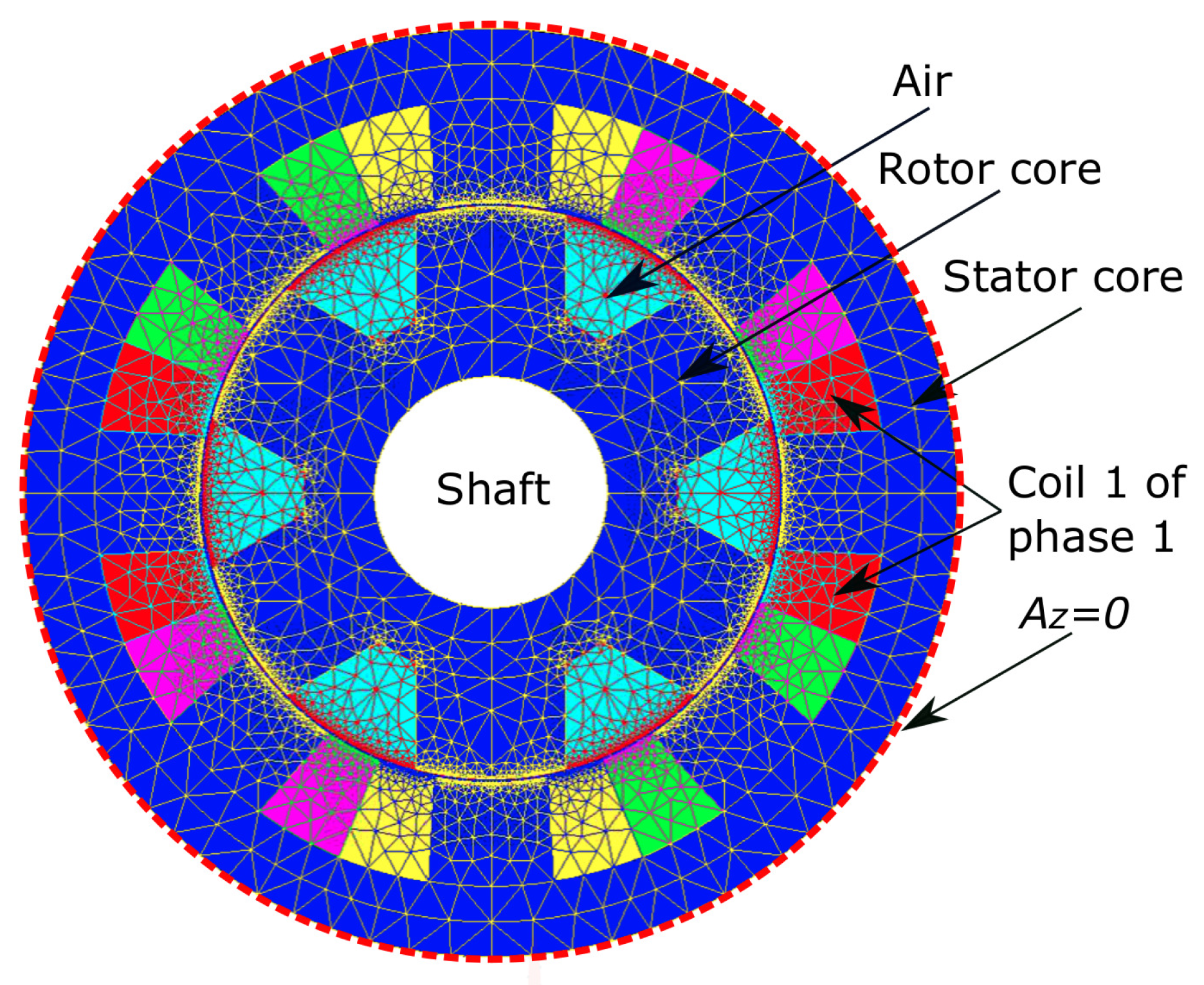
The SRM under study has $N_s=8$ stator poles, $N_r=6$ rotor poles with $m=4$ phases, as shown in Figure 1. The parameters of this motor are shown in

Table 3. Parameters of the studied 8/6 SRM.

Parameter	Value
Power	550 [$\mathrm{W}$]
Speed range	0–1500 [RPM]
Voltage	$300\left[\mathrm{V}\right]$
Inertia moment	$0.00149257\left[\mathrm{k}\mathrm{g}{\mathrm{m}}^2\right]$
Phase resistance	$4.2048\left[\mathsf{\Omega }\right]$
Leakage inductance	$0.5996\left[\mathrm{m}\mathrm{H}\right]$
Number of turns per phase	284

. The FE model was implemented in the commercial software Altair Flux 2D [29] and solved using the 2D transient magnetic solution. The mesh has 24,048 nodes and 12,000 second-order triangular elements. A Dirichlet boundary condition $(A_z=0)$ is enforced at the shaped curves bounding the 2D SRM model (see Figure 1) to ensure a unique solution of (25). The total number of unknowns in the FE model are as follows: 24,048 nodes minus the number of nodes at the boundary where the potential is known $(A_z=0)$.

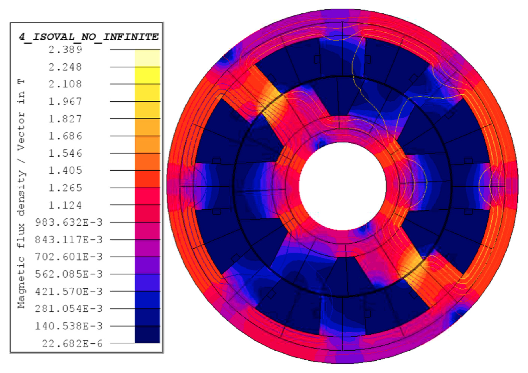
Figure 2 shows the magnitude distribution of the magnetic field density $B\left(A_z\right)$$\left[\mathrm{T}\right]$ and flux lines for an operation of 157 $[\mathrm{rad}/\mathrm{s}]$ and a load torque equal to $1.5$$\left[\mathrm{N}\mathrm{m}\right]$ for the open-circuit fault in phase 1. At time $1.2074$$\left[\mathrm{s}\right]$, the current has its maximum value of $5.92$$\left[\mathrm{A}\right]$. In the figure, the magnitude of the magnetic flux density is related to different color shades. The highest values of $B\left(A_z\right)$ are represented in yellow, and the values close to zero in dark blue. It is worth noticing that some regions reach magnetic saturation with maximum values of $B\left(A_z\right)$ equal to 2.38 $\left[\mathrm{T}\right]$. This situation is not present under healthy conditions and reflects the importance of using a VTB based on FE models to reproduce the nonlinear motor behavior, which is an aspect that cannot be represented by model (3).

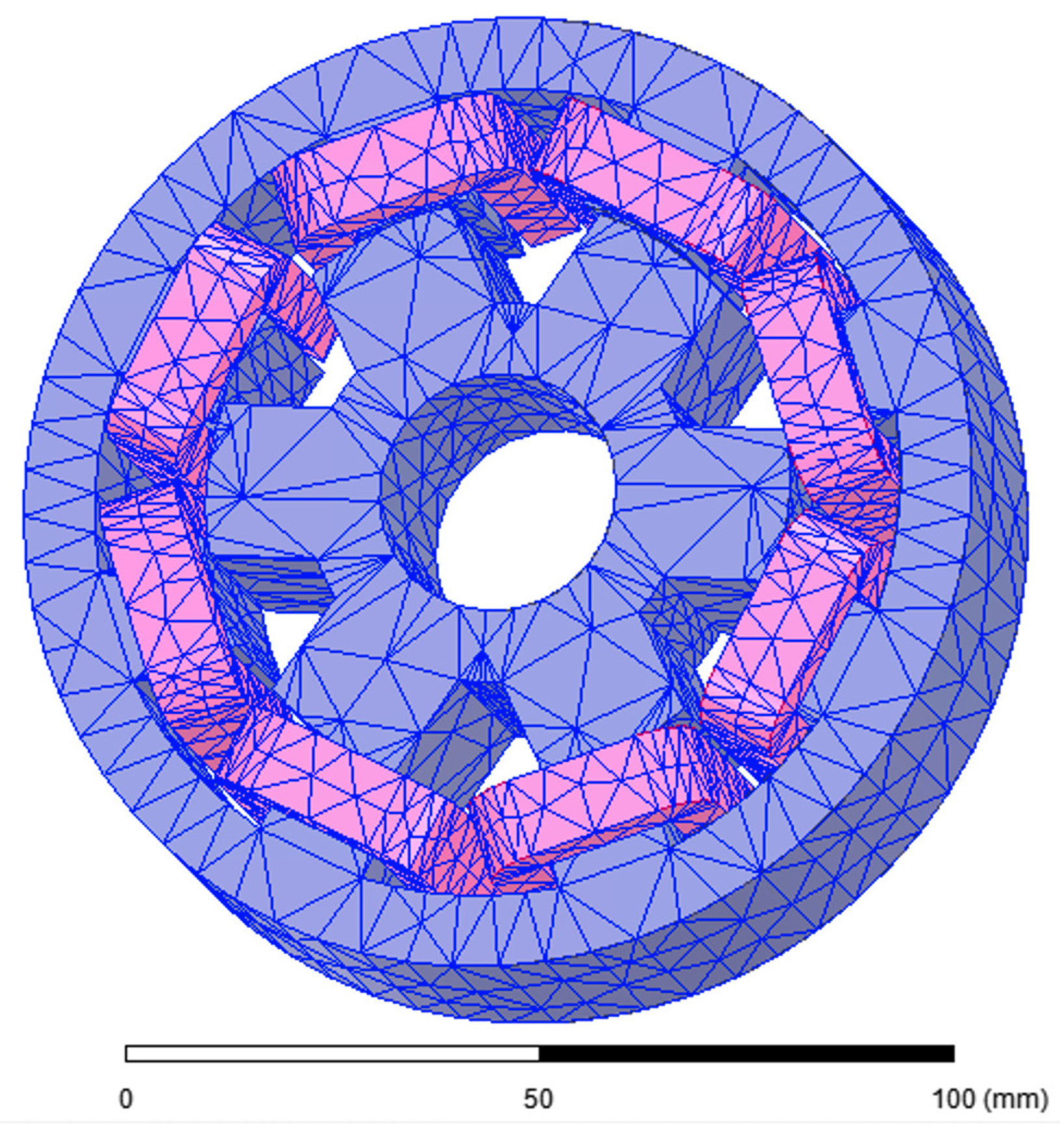
Validation of the 2D FE Model

3D FE computations were employed to validate the 2D FE model of the SRM used in this work and explained at the beginning of Section 4. We implemented the 3D FE model in the commercial software Ansys Maxwell 3D [48]. The 3D geometry and mesh are shown in Figure 3. The mesh has 15,916 tetrahedral elements.

A magneto-static analysis was performed at different values of current in phase 1 only and changing the rotor position from ${22.5}^{\circ }$ to ${202.5}^{\circ }$. The rotor position equal to ${22.5}^{\circ }$ correspond to the unaligned position for phase 1. Figure 4 shows the self-inductance in phase 1 for values of current of 3 [A], 6 [A], 9 [A], 15 [A], 24 [A] y 36 [A]. In this Figure, a good agreement can be seen between the results of 2D and 3D models, even for saturation conditions at excitation levels of 24 [A] and 36 [A]. This comparison of results gives certainty that the 2D FE model is reliable and can be used to analyze the open circuit fault. Advantages of 2D models: lower computational cost and faster simulations.

5. Validation of the FD System

To validate the FD system, a comparison with a fast Fourier transform-based method by [11], which will be referred to as the FFT method, will be made in the following. In all the cases, operation is at $70[\mathrm{rad}/\mathrm{s}]$ with a load torque equal to $0.75\left[\mathrm{N}\mathrm{m}\right]$.

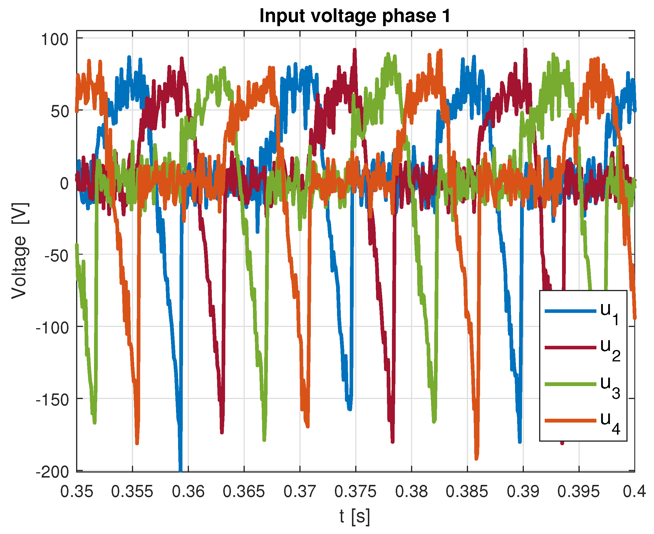
Fault cases: Phase 1 open, phases 1 and 2 open and phases 1 and 3 open. In all fault scenarios, the motor is working under steady-state operation at the moment of fault.

The gains for the PBC controller are $a=b=3000$, $\mathit{K}={[5,5,5]}^T$. The gains used in the EKF are $\alpha =15$, $Q=30{\mathit{I}}_6$, with ${\mathit{I}}_6$ the $6\times 6$ identity matrix and $W=1$. The time step was $T_s=0.1$ [ms], with Runge–Kutta fourth-order method. White Gaussian noise with variance $s^2=100$ was added to the input voltage signals. The corrupted signals, shown in Figure 5, approximately represent the typical and realistic signals that are acquired during the operation of a motor. However, in order to define the uncertain input parameters a sensitivity analysis must be carry out. This analysis can be made using the tools proposed in [49] where the influence of noise and uncertainty can be rated to understand how it affects the input.

To implement both methods, the bus current is defined as

$$i_{bus}=i_1+i_2+i_3+i_4,$$

(29)

which corresponds to the excitation bus current as defined in [11].

5.1. FFT Method

The FFT method by [11] is based on the measurement of the bus current that is analyzed to obtain its spectrum. In normal operation, the bus current spectrum only shows the amplitude harmonics for the DC component and the frequency of the bus current, $f_{bus}$, where the frequency for the bus current is calculated as

$$\begin{array}{cc}\hfill f_1& =n{N}_r/60\hfill \end{array}$$

(30)

$$\begin{array}{cc}\hfill f_{bus}& =m{f}_1,\hfill \end{array}$$

(31)

with n the motor speed in RPM and $f_1$ the fundamental frequency of the phase current. When a fault occurs, other harmonics appear with amplitudes, $A_{f_1}$ and $A_{f_2}$, which are normalized to obtain the signature (pattern) for a given fault as shown in the following expressions:

$$\begin{array}{cc}\hfill A_1^{*}& =A_{f_1}/A_0\hfill \end{array}$$

(32)

$$\begin{array}{cc}\hfill A_2^{*}& =A_{f_2}/A_0,\hfill \end{array}$$

(33)

where $A_0$ is the DC component amplitude. The diagnostic is made by comparing the values of amplitudes $A_1^{*}$ and $A_2^{*}$ with an interval value related to the fault case.

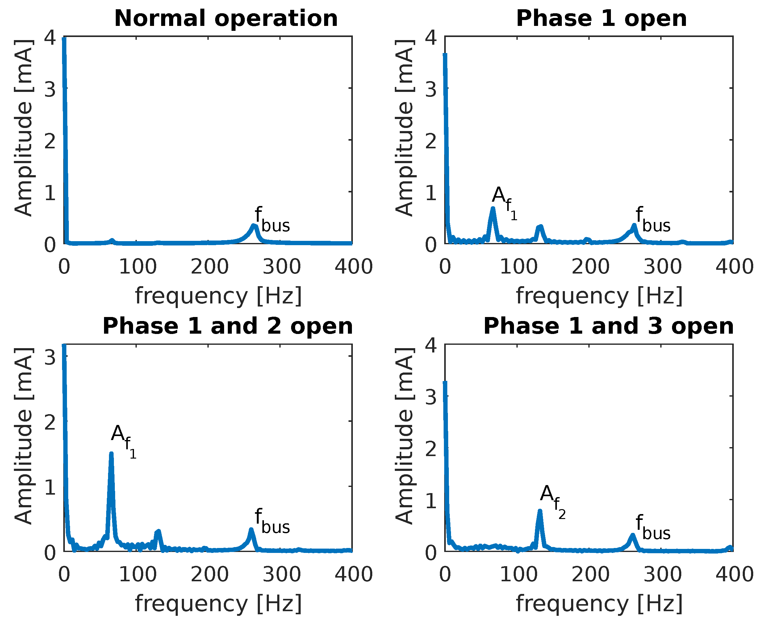
The results for normal operation and three faults cases are collected in Figure 6. This figure shows the method can detect the faults correctly. For faults in phase 1, and phases 1 and 2, harmonic $f_1$, at $64\left[\mathrm{Hz}\right]$, must be present in the spectrum. On the other hand, for a fault in phases 1 and 3, harmonic $f_1$ is not present but harmonic $f_2$ at $130\left[\mathrm{Hz}\right]$ appears. In this case $f_{bus}=264\left[\mathrm{Hz}\right]$.

5.2. FD System

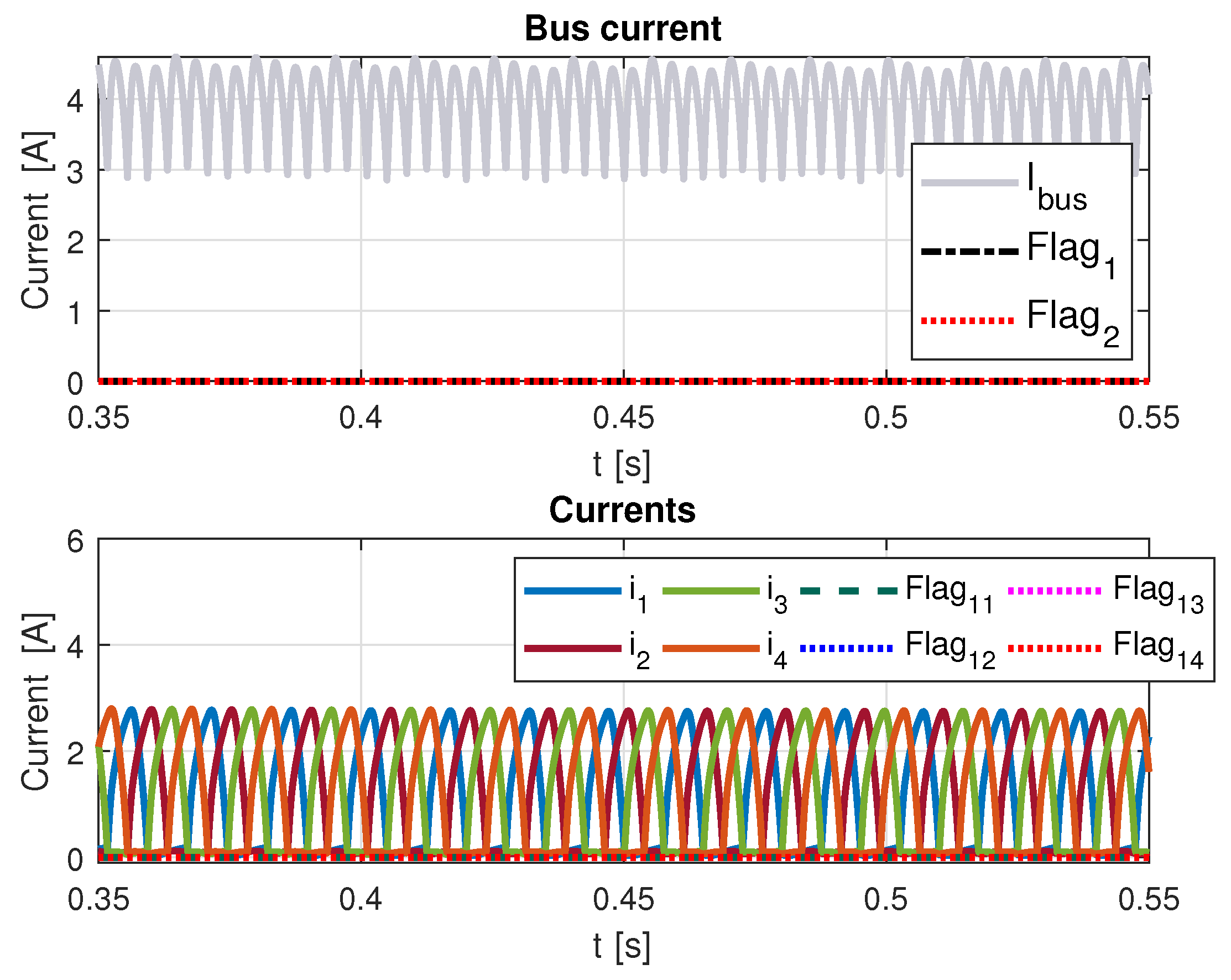
For the proposed detection method, Figure 7 shows an operation without fault, where the top figure includes measured bus current, flag 1 and flag 2. Both flags are equal to zero in the absence of a fault. The bottom figure shows four stator currents and their respective flags at zero. It must be noted that in the bottom parts of Figure 7, Figure 8, Figure 9 and Figure 10, phase currents are included to show the moment of the fault.

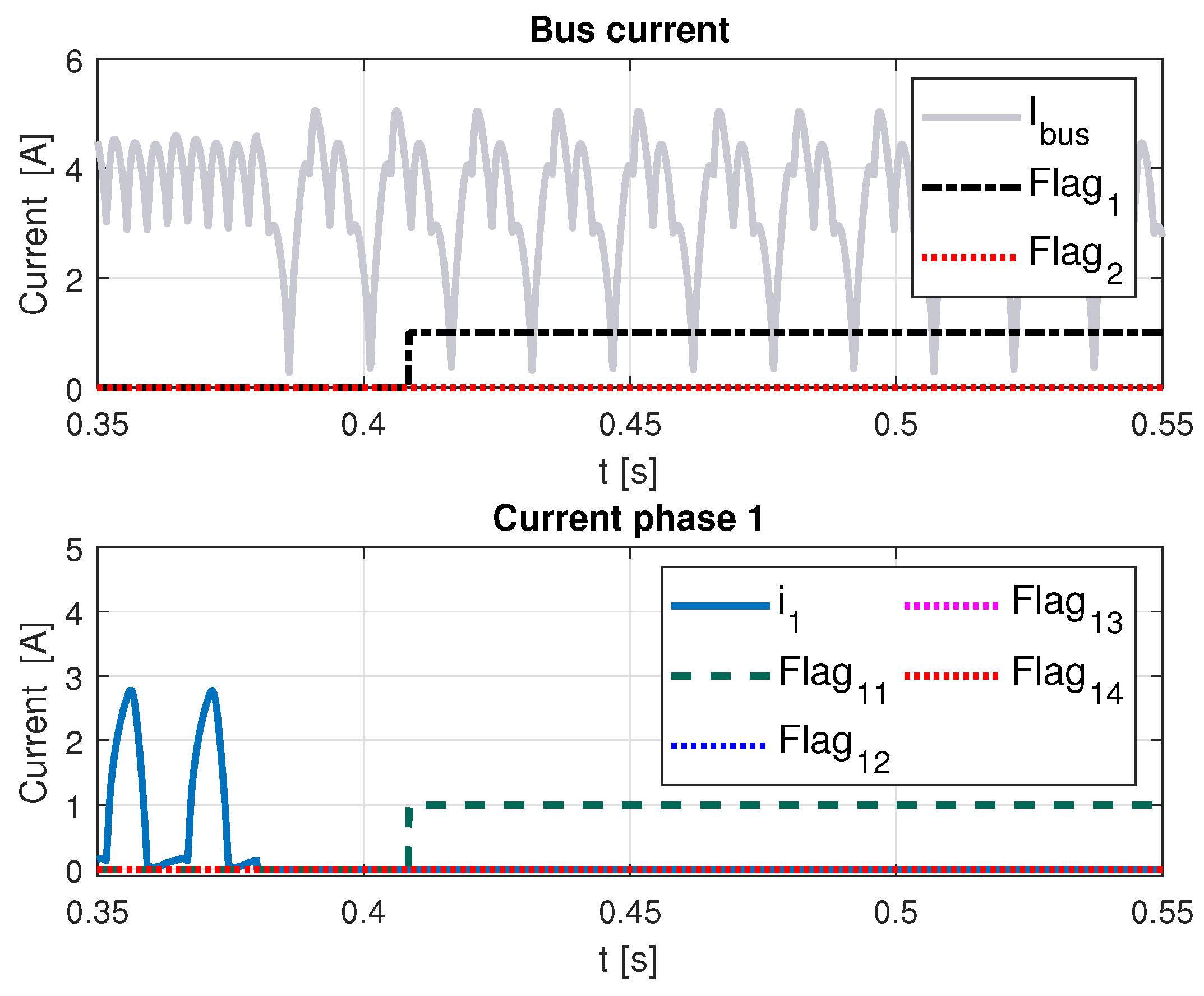
For Figure 8, flag 1 is activated some time after the fault indicating there is a one phase fault. In the bottom figure, the current in phase 1 becomes zero after a fault occurrence, and flag 11 is properly and quickly activated.

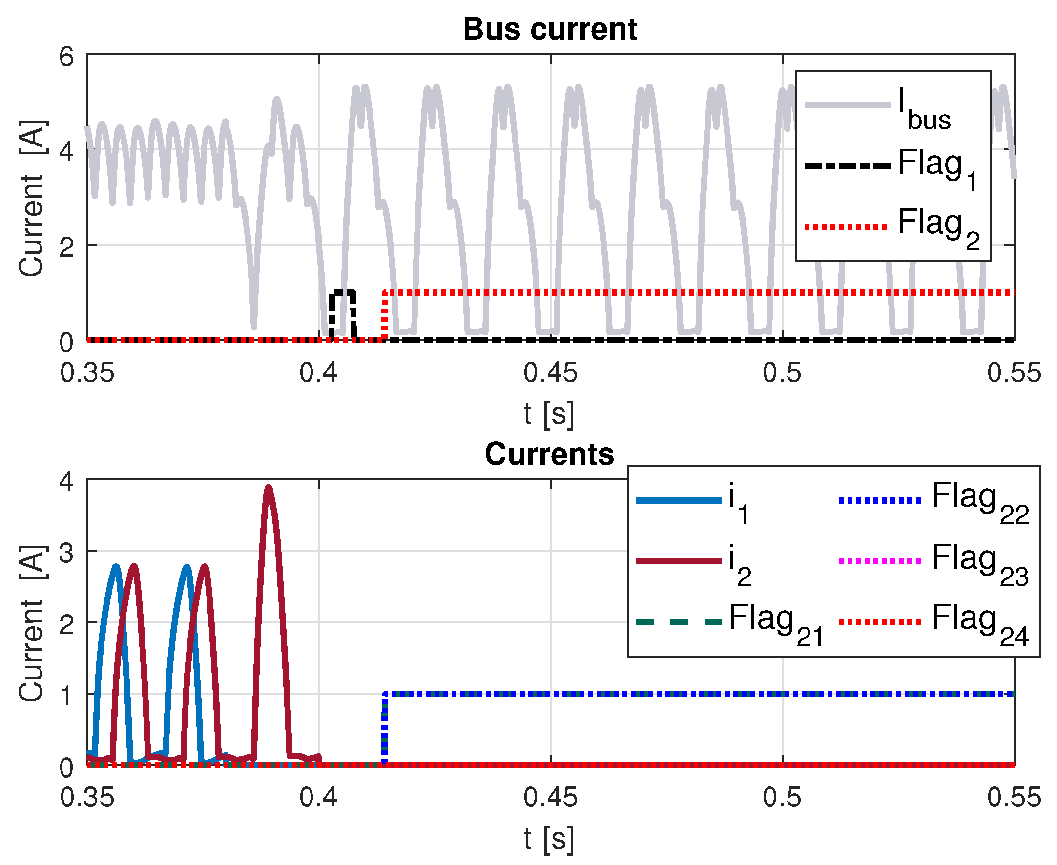
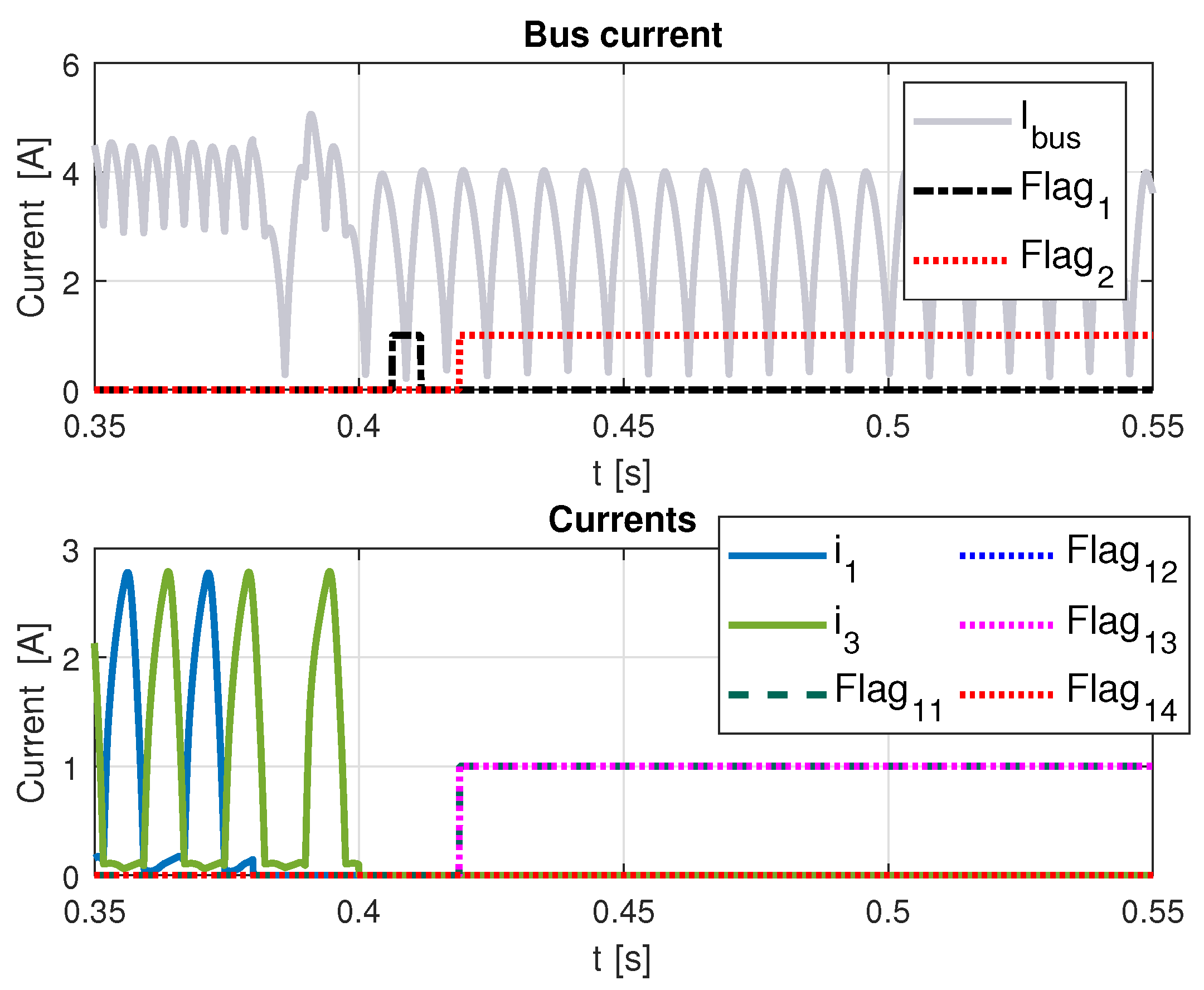
In Figure 9, faults in two consecutive phases occur at different times, one after the other. In this case, flag 1 activates for a brief moment, indicating a one-phase fault; however, once phase 2 fails, flag 2 is activated accordingly. The bottom figure shows flag 21 and flag 22 are different from zero to indicate the faulty phases.

Finally, Figure 10 shows faults in non-alternating phases (1 and 3) at different time instants. In this case, flag 1 and flag 3 also activate correctly by indicating a one-phase fault and two-phase fault as the phases become zero. In this case, the figure bottom shows flag 21 and flag 23 are different from zero to indicate the faulty phases.

Once the fault occurs, in all cases the controller increases the current in the remaining healthy phases to try to maintain speed at its desired value. Loss of one phase also leads to an adjustment to reach desired torque. This is quickly compensated by other phases to deliver the required instant torque value. In addition, current in the remaining phases is greater in the winding adjacent to the phase in open circuit.

6. Discussion

This section presents a qualitative comparison between the two methods. The similarities between these methods are included first, and later the stronger characteristics of each method are mentioned.

It is true for both methods that, as stated in the previous section, they were able to correctly identify the faults and faulty phases for the three cases. In addition, both methods only need the information of the bus current sensor, the stator and rotor poles, and the phases number. Neither method requires additional circuitry or more sensors.

Regarding the differences, in [11] three different locations are defined for the bus current sensor for the FFT method, while for the FD system the sensor must be placed so it senses the excitation bus current. Another important difference is that, the FD system can detect faults in real time. It has information of the fault time for every faulty phase, while the FFT method needs an additional algorithm to indicate the moment of fault. The FFT method, however, has a diagnosis time of one current period $T_{ph}=1/f_1$, while the FD system has a diagnosis time of approximately $5T_{ph}$. Moreover, the FFT method is valid on a wider speed interval, while the FD system is only valid for low speeds below the base speed. A summary of each method’s characteristics is given in

Table 4. Comparison of fault detection methods.

Characteristics	FD System	FFT Method
on-line	yes	no
number of current sensors	one	one
bus current locations	one	three
detection time	$5T_{ph}$	$T_{ph}$
robustness	high	high
cost	low	low
fault diagnosis	easy	easy

.

In conclusion, the FFT method is quicker, but it needs another location algorithm to define the time of fault, and works in an wider speed interval. While the FD system proposed is on-line, it detects the faulty phase in real time, and does not need to store any data to give a diagnosis.

7. Conclusions

The article presents an on-line fault diagnosis method for open-phase faults in switched reluctance motors using only one current sensor. The FD system can detect and identify all possible fault scenarios in real time for low speed operation using only measured bus current and angular position signals. The fault detection system calculates analytical relations and the threshold in a time window to avoid storing unnecessary data. Consequently, this method does not spend excessive computational resources. Although a relatively simple model of the motor is used for control and observer design, a good performance is obtained in speed regulation and in the fault diagnostic system. A virtual test bench of the SRM was used to test the proposed fault diagnosis method under different fault scenarios. The advantage of testing in this way is the possibility of evaluating various diagnostic systems with signals generated by models very close to real motors. In this sense, virtual tests become essential in industrial environments where the evaluation of diagnostic systems is required before being implemented in reality. The reason: damaging machines to test fault detection systems is expensive.