Artificial Immune Systems: An Overview for Faulting Actuators

Abstract

This paper reviews Artificial Immune Systems (AIS) that can be implemented to compensate for actuators that are in a faulted state or operating abnormally. Eventually, all actuators will fail or wear out, and these actuator faults must be managed if a system is to operate safely. The AIS are adaptive algorithms which are inherently well-suited to these situations by treating these faults as infections that must be combated. However, the computational intensity of these algorithms has caused them to have limited success in real-time situations. With the advent of distributed and cloud-based computing these algorithms have begun to be feasible for diagnosing faulted actuators and then generating compensating controllers in near-real-time. To encourage the application of AIS to these situations, this work presents research for the fundamental operating principles of AIS, their applications, and a brief case-study on their applicability to fault compensation by considering an overactuated rover with four independent drive wheels and independent front and rear steering.

1. Introduction

With the increase of robotics designed to work in hazardous environments, there has been an increased focus on ensuring systems can either continue operating or “limp home” when actuators fault. This field, Fault-tolerant Control (FTC), is an extremely active area of research and is ever expanding [1]. One of the emerging areas of study for FTC is bioinspired algorithms such as evolutionary algorithms and genetic algorithms. One of the genetic algorithm variants, the Artificial Immune System (AIS), has several of the traits that would be beneficial in FTC including adaptability to new situations and a memory of previous solutions. Historically, these algorithms have been limited due to their computational intensity. Advances in computation have allowed these algorithms to become feasible. An overview of genetic algorithms and AIS theory, methods, construction, and application in FTC is presented here.

Before diving into the AIS, the backbone of the genetic algorithm will be provided. This will be done with the binary genetic algorithm first, as it is generally the simplest to explain. Because actuator faults are often nonbinary, real-world applications require an extension of the binary genetic algorithm to use real numbers. These real-value genetic algorithms utilize floating point numbers and require some important modifications to the genetic algorithm to be functional. Once the fundamentals of a real-valued genetic algorithm are laid out, the AIS can be discussed in detail.

1.1. Background on Fault-tolerant Control

FTC is an active field of study in part due to the inherent limitations of many methods involved. A complete discussion of common FTC methods can be found in the literature in survey terms [1,2,3]; in application specific terms, such as aircraft [4,5]; and in methodology terms, such as gain scheduling [6]. To demonstrate the applicability of the AIS in FTC, several common FTC methods will be discussed: multiple model controllers, gain scheduling, and sliding mode controllers, and model predictive controllers. The main target of this particular application is multiple model controllers and model reference adaptive control (MRAC), which attempt to force the system to behave like a desired reference system [7]. This paper does not consider fault detection or diagnosis.

Multiple model (MM) controllers, also known as discontinuous controllers, have shown some limited success. The system is given an a priori set of controllers. For FTC, these different controllers typically compensate for different faults that can occur. For a very simple example, a robot could be given a controller that compensates for each actuator failing. The controller that corresponds to a known fault can be activated with minimal time and effort once the fault is detected. For a simple example of this, consider a grid-based robot that can travel forward and perform 90-degree rotations to the left and right. When the robot is facing north and wishes to move east, it would rotate right to face east and then move forward. If this robot were to fault and be unable to rotate to the right but could still rotate left and move forward, a multiple model structure could be implemented to overcome this. The controller would dictate that when the robot needs to move to the right, it will perform three 90-degree rotations to the left and then move forward.

Recently, a MM controller has shown the ability to control a four wheeled vehicle in the presence of actuator faults at low speed [8]. The vehicle tested here had four independent drive wheels that were connected by two steering motors. This allowed each wheel to provide a propulsive effort, while the front wheels were aimed in one direction and the rear wheels were aimed in another. When a short is detected in the front drive wheels, the controller switches from all-wheel drive to rear-wheel drive. When a fault is detected in the rear drive wheels, the controller switches from all-wheel drive to front wheel drive. This prevents the system from behaving unexpectedly as the error can be side-stepped through redundant systems.

MM controller systems are limited in that, on their own, they cannot adapt to errors that are outside the errors they were tailored for. That is, for the vehicle example, if a fault occurred in the steering motors or in both wheels on the left side, the MM controller would fail. An exhaustive search method can be attempted to generate more models, such as in the work of Cully, Clune, and Mouret [9]. These possible candidates are generated by trialing all controller configurations ahead of time. When a fault is detected, the best model is selected based on an intelligent search of the a priori controller configurations. This expands the functionality of the system, but it still does not have the ability to account for all faults and it requires extensive computation before any improvements can be made to the faulted system. A simple hexapod robot required a 2-week computation to generate all possible model configurations [9].

While these controllers lack versatility, they excel in situations where the failure modes are known. If a failure is known to be likely, then developing a controller beforehand can save valuable time when the error is detected. Similarly, if a given component is guaranteed not to fail, then no effort or computation needs to be spent on considering the possibility of it failing. Their use of a priori information is excellent, but they have difficulty adapting to situations outside their initial knowledge base.

Other switching-type controllers include gain-scheduling (GS) and sliding mode (SM) controllers. GS controllers have shown the ability to easily correct for errors that follow anticipated error paths within linear systems. These systems typically use linear parameter varying (LPV) controllers; however, they can be coupled with eigenvalue assignments to allow for guarantees of stability under total failures that cause nonlinear behaviors [10]. Sliding mode controllers have shown success with theoretical FTC systems, but have had difficulty in practice. This is due to “parasitic dynamics” or high frequency noise in the plants that are generally considered negligible when designing a controller [11]. By incorporating an asymptotic observer, these parasitic dynamics can be accounted for and filtered out of the controller. This allows the SM controller to guarantee stability without needing to identify the cause of the fault, perform system identification online, or redesign the controller online [11]. However, the SM controller requires the plant model to be static while compensating for the fault and it cannot deviate too significantly from the design point or operating envelope [6]. Additionally, the nonlinearities can cause the system to break down if unexpected nonlinear behaviors are introduced [1]. In practice, the physical system can become more complex after an error and errors can compound one another. Thus, these controllers have the ability to adapt, but have trouble doing so in dynamic environments.

A model predictive (MP) controller is designed to deal with dynamic plants, anticipating how they will change over time. Because the system deals with dynamic plants, a failure can be seen by the controller as a change in the plant, assuming the failure is not too sudden for the controller. For faster failures, where the controller sees the change as a large discontinuous change, the controller requires a model of the fault or the system after the fault [12]. Recently, research on MP control has shifted toward nonlinear and quickly changing systems. MP control can account for certain nonlinearities entering a system by injecting the nonlinear effects into the controller and then compensating for them. Unfortunately, this typically has to be done externally to the controller and can only give bounded input-bounded output (BIBO) stability in many cases [13]. It should be noted that the situations where these nonlinearities can be accounted for are fairly limited at the current stage of the research.

In general, model prediction lends itself very well to FTC problems, but it has several limitations that are particularly difficult in this case. First, existing nonlinearities in system dynamics can make it difficult for the system to adapt to new nonlinearities caused by a fault. Secondly, for certain fault cases, the controller cannot adapt to errors on its own. Instead, it must rely on an external component to give it new input. Lastly, these systems have difficulties with compounding errors and very fast changes.

1.2. Background on Bioinspired Algorithms

When discussing bioinspired algorithms, most researchers are more familiar with the Artificial Neural Network (ANN) than the Artificial Immune System (AIS). Instead, this paper will focus on the AIS as opposed to the ANN. Both are artificial models of complex biological systems: with the AIS modeling the vertebral immune system and the ANN modeling the brain. Significantly more work has been invested in researching the ANN than the AIS: “Though ANNs are well established techniques and are widely used, AISs have received very little attention and there have been relatively few applications of the AIS” [14]. This means that there are likely existing applications where the AIS would be preferable to the ANN but are not currently being used. For example, the ANN typically uses a central control node to mimic the centralized nature of the brain. The AIS can be implemented this way, but the immune system is distributed throughout the body and so is extremely well suited to applications with distributed systems and swarm robotics.

Both the ANN and the AIS are extremely computationally heavy. Cloud and distributed computing have allowed these bioinspired algorithms to become feasible solutions by increasing the number of calculations that can be done at any moment. For the AIS, this can increase the speed of the response since all computationally intensive portions of the algorithm can be run independently, or parallelized. This parallelization has been key to utilizing the computational advances for the ANN and AIS. As these technologies improve, the AIS and ANN will become faster. Cloud computing services such as Google Cloud, Amazon AWS, and Microsoft Azure allow incredibly heavy computations like those involved in the ANN and AIS to be performed quickly without large investments from individual companies or researchers. On the distributed side, inexpensive hardware advances can provide comparable or significantly improved performance over desktops and laptops with extremely small form factors and power requirements for independently deployed systems [15]. Examples include $99 NVIDIA Jetson Nano for AI applications like ANN, and the $75–150 Google Coral Edge TPU for distributed applications like the AIS [16,17]. Whether done in a centralized cloud or distributed system, these computational advances are enabling the AIS and ANN to be tested in applications where they were previously seen as too slow, such as in FTC.

The two largest factors preventing the AIS from becoming more common are the complexity of the algorithm for those implementing them [14] and the long time periods required for convergence. As the technological advances allow the algorithms to be computed faster, the AIS will become more available. Some of the first applications will be for slow systems, such as maritime vessel operations. The research in this area indicates significantly larger timescales available for computations [18].

While bioinspired algorithms such as the ANN are used extensively in fault detection and diagnosis [19], especially through deep learning [20], this paper will address fault-tolerant control regardless of whether detection or diagnosis is included. The AIS that will be discussed could incorporate fault detection or could be run continuously, as in the example provided in Section 3. Diagnostic conclusions could be drawn from the controller solution provided at the end of the algorithm, but these typically require extensive performance data. ANNs are better suited to this analysis and interpretation phase than the AIS.

One of the key differences that recommend AIS over ANN in this application is the way the systems are designed to respond. ANNs are generally utilized for postprocessing large datasets or interpreting new information based on the knowledge gained from these sets. This results in a large time delay between inputs and outputs, but initial outputs that are of high quality. Essentially, the ANN needs to wait and think, even in FTC implementations [21]. On the other hand, the AIS is designed to develop an immediate output which is of questionable quality which improves over time.

In an emergency, the system cannot afford to wait and think. It needs to respond quickly, even if the response is suboptimal. For example, if a UAV swarm is no longer responding as expected, the UAVs cannot wait while a centralized system identifies the cause and the solution. The UAVs need to attempt some sort of compensation immediately. Like the cells of the vertebral immune system, the distributed nature of the swarm allows each UAV to test compensation methods individually. The performance of each UAV can inform future compensation for the group. Between the distributed nature of the AIS and the continually improving response, the AIS is better suited for FTC than the ANN in certain scenarios.

2. Genetic Algorithms

Genetic algorithms were first introduced in the early 1960s [22], and have demonstrated historical success at solving a variety of problem [23,24]. They also have a long track record of being able to function in suboptimal environments [25]. As a member of the family of evolutionary algorithms, these algorithms attempt to mimic Darwinian evolution. However, the key feature that differentiates these algorithms from other evolutionary ones is their focus on paralleling the mechanics of genes and DNA on a cellular level.

Modern biology classes cover genetics and the basics of cellular reproduction with enough detail for this paper. The core functionality is as follows; within a certain population of organisms, the individuals that are most suited to survive in the current environment, the fittest, can reproduce and generate the most offspring. The genes that make those individuals the fittest ones will be passed along to the future generations. Except for rare circumstances, such as a suddenly changing environment, this means that the overall fitness of the population will increase and eventually an optimum individual will be created. There are many important caveats to the above that are not readily apparent in nature but become critical in writing these algorithms. To discuss these, the simple binary genetic algorithm will be discussed.

2.1. The Binary Genetic Algorithm

When all control parameters in a problem can take one of two values, the binary genetic algorithm has can consistently find an optimal solution. Each control parameter for the problem is represented as a bit, which can either be high (value of 1) or low (value of 0). This means that a binary string or array containing a bit for each control parameter can represent a configuration of the control parameters. These strings are often termed candidates or candidate solutions. Within the biological model, an individual competes within a population for the right to reproduce based on its fitness, which is dictated by the effects of its genes. The binary genetic algorithm begins the biological parallel by considering each candidate binary string as an individual organism. The bits within the strings serve as the genes, while a collection of these individuals is considered a population.

To generate a reasonable solution to the optimization problem, the population must be sufficiently large. If the population is too small, there is insufficient diversity to ensure the solution generated is a global optimum. The genetic algorithm shares many traits with common hill-climbing algorithms such as greedy attraction toward local optima and an inability to leave local optima if not implemented correctly. Required strategies exist for preventing local optima such as increased mutation or migration, which will be discussed later. However, the cleanest method to ensure a solution closer to the global optimum is produced in a reasonable timeframe is to use a sufficiently large population. The literature recommends a population that has ten times as many individuals as there are variables to be optimized.

The population in a genetic algorithm is typically created at random. As the population is generated, the major concerns that often arise are clustering away from the global optimum and a lack of genetic diversity. When the population is clustered away from the global optimum, the algorithm will take significantly longer to complete. If the population has insufficient genetic diversity, then the system cannot generate a reasonable solution through recombination of the individual genes in the population. With enough time, the optimum can be found but this relies too heavily on random mutation.

Alternative heuristic methods can be used to attempt to mitigate these issues. These can include the use of scatter patterns [26], orthogonal arrays [27,28], and initial testing to determine probable optima [29]. These approaches are best suited to continuous or real-valued genetic algorithms [26,27], but can function in discrete or binary situations [27], especially in manufacturing environments [28]. These studies indicate that, while these approaches provide a good distribution across the possible configurations of the input parameters, they are equally susceptible to missing global optima and being drawn into local optima. The literature has some debate on the matter so many applications use either a randomly generated population or a population that has a randomly generated population augmented by a heuristically generated population.

To determine which candidates in the population should be allowed to pass along their genes, the fitness of each candidate must be determined. The fitness is calculated through some pre-determined heuristic. This measure follows directly from the standard cost function or objective function found in optimization problems [30]. At times, these functions are augmented through the addition of other terms to allow the algorithm to function appropriately [30]. This augmentation could take the form of a penalty for a population that is too uniform, a bonus for a candidate that has a trait not found in the rest of the population, increasingly complex terms that are introduced as the solutions gets more successful [31], or environmental constraints that are introduced over time [32].

Once the fitness of the individuals has been determined, they can be used to create a new generation of individuals. To do this, the best candidates need to be selected. The selection of these individuals for reproduction can be done through a variety of different methods. The most popular are fitness proportionate selection and stochastic uniform sampling.

Fitness proportionate selection is commonly termed “roulette wheel selection” due to its mechanics. The total fitness of the population is calculated as the sum of the fitness values of every individual in the population. The total fitness can be envisioned as a roulette wheel where each wedge of the wheel corresponds to an individual in the parent population. The width of each wedge is determined by the percentage of the total fitness that can be attributed to each individual. When a parent needs to be selected, the roulette wheel is “spun”. Each individual has a probability of being selected equal to the percentage of the wheel occupied by its corresponding wedge. An example using this selection mechanic will be provided in the next section.

Stochastic uniform sampling uses the total fitness of the population and a single random variable to determine which individuals will reproduce. The fitness of the individuals is again summed and the percentage of the fitness that corresponds to each individual is again calculated. However, instead of each individual being drawn randomly from a wheel, one random number is drawn as the starting point for the selection of all individuals along a number line. This number must be less than or equal to the step size. The number line is generated by concatenating the fitness of the individuals in descending fitness order. Consider a 3-individual population that has individuals α, β, and γ. If the fitnesses of α, β, and γ are 26, 8, and 10, respectively, the number line would be 44 units long. The first 26 units correspond to α, units 27 through 36 correspond to γ, and units 37–44 correspond to β. The selection process then takes evenly sized steps through the entire fitness of the algorithm. At each step, the corresponding individual is selected. The step size is determined by dividing the total fitness by the number of individuals needed. For the example above, assuming four individuals are to be selected, the step size should be 11. Assume the random number indicating the starting point is 8. The first individual then is the one with a fitness corresponding to unit 8, meaning α is selected. The step size is added to the random number, generating the value 19. The individual with a fitness corresponding to unit 19 is still α, so it is selected a second time. Again, 11 is added to the random value, generating 30. Since 30 is between 27 and 34, γ is now selected. The step size is added again, generating 41, indicating that β should be selected. Thus, the four selections are: α, α, γ, and β. These four selections are randomly paired for reproduction.

The main advantages of stochastic uniform sampling over fitness proportionate selection are that only a single random number needs to be generated and individuals with very low scores are more likely to be chosen. Computationally, the reduction in random numbers slightly decreases the time required for the algorithm. Additionally, when an individual or small cluster of individuals dominate the overall fitness, the fitness proportionate selection process will bias the selection process away from the smaller values. The stochastic uniform sampling will give less fit individuals a better chance of being selected at least once [33].

After selection, the chosen candidates are allowed to reproduce and generate a child population through crossover. In crossover, a new binary string is generated through a combination of two other binary strings. To keep with the biological parallel, the pair of binary strings is called the parents and the new binary string is called the child. The most common methodology to create the child is for the first portion of the child to be copied from one parent and the second portion to be copied from the other parent. This is called single-point crossover. To accomplish this, a random number is generated which is approximately the length of the binary string. This random number indicates the location, or locus, where the DNA source switches from one parent to the other.

The literature includes some minor debate about whether to allow the locus to occur at the very front or very back of the string [34]. If this happens, the child will be identical to one parent and take no traits from the other. Another mechanic, elitism, exists to allow the best parents to be passed from one generation to the next. However, allowing the locus to extend to the limits of the string allows lesser parents to be passed directly into the child population at random. Since this adds candidates that are not redundant individuals, most applications allow it. That is, for a 10-bit string, a random number is generated from zero to ten. If the number is between 1 and 9, inclusively, then the child will be a hybrid of the two parents as crossover after gene 1, gene 9, or any gene in between will have components from both parents. If the value is 10, it will be a direct copy of the first parent, and if the value is 0, it will be a direct copy of the second parent.

Single-point crossover is acceptable for most applications, but multiple-point crossover can be used. In multiple point crossover, multiple numbers are randomly generated for the loci. As the algorithm generates a child, it switches sources between parents at each locus. Two loci are the most common application, but three or more loci can be used in longer strings. Multiple loci force the children to be more hybridized at the expense of decreased diversity. Because the candidates are drawn to the average of the parents, there is a smaller chance to end up closer to one parent or another, which leads the overall population to have less diversity. Because of this, three or more loci are infrequently seen.

After the crossover children have been produced, mutation can alter the children’s genes. Mutation is a key factor that ensures a genetic algorithm has theoretical guarantees of optimality and prevents the algorithm from getting drawn into a local optimum [34]. In mutation, any number of bits can be flipped from 1 to 0 or from 0 to 1. Mutation algorithms need not be complicated. Often a small percentage of individuals is randomly selected for mutation. This mutation percentage depends on the application, but values between 1% and 5% are common, with values up to 10% in certain applications. The children selected for mutation are chosen at random to prevent any bias in the algorithm. Once a child is selected for mutation, the number of bits that are flipped is determined by the application and the mutation percentage. If the mutation percentage is high, a large number of children will be mutated, so the number of bits to be flipped is held low and vice versa. Increased mutation rates increase the diversity of the child population at the expense of computational time required to converge to a solution. Therefore, tuning the mutation rate is critical in any application.

Crossover and mutation are not used to generate the entirety of the child population in most applications. Any remaining candidates can be generated through elitism and migration. Elitism allows the best candidates to be passed to the child population untouched. If elitism is used, the elitism rate is kept low, typically ~5%. This low value is typically sufficient to prevent the best candidates from being lost due to random selection without degrading the speed of the algorithm unduly. The elite children can either be defined as the best individuals, or the best unique individuals. If the unique individuals are chosen, the algorithm may have convergence problems in the final stages as the population becomes more homogeneous.

Migration allows randomly generated individuals to be injected into the child population directly. Various methods are used to implement migration. The most common are to always include a small percentage of every child population as random individuals, or to inject new migrant candidates at key stages of the algorithm. When adding random individuals to every child generation, the population stays diverse at the expense of time to converge. When injecting new migrants into the algorithm at key stages, the injection can either occur when a change in the problem is detected, i.e., the goal has changed or shifted or when the population has begun to converge to an optimal value. In both cases, the migration allows a sudden spike in diversity to ensure the population trends toward the global optimum instead of a local one.

Example Binary Genetic Algorithm

To demonstrate the mechanics of the binary genetic algorithm, consider a complex but unknown piping system with ten valves that control the output flow of a tank. If the output flow of the tank is to be maximized through opening and closing the valves via binary actuators, such as solenoids. A binary genetic algorithm could be used to determine the optimal valve combination. Each of these valves is essentially a Boolean variable since it can either be open or closed, but not something in between. Therefore, the combination of the valves can be represented by a binary string such as the combination

$$\mathbf{A}=\left[\begin{array}{cccccccccc}0& 0& 1& 0& 0& 1& 0& 0& 0& 1\end{array}\right],$$

(1)

where valves one through ten are represented by entries one through ten, respectively. A high value (1) represents an open valve, while a low value (0) represents a closed valve. Equation (1) represents a combination where only valves 3, 6, and 10 are open. The fitness of $\mathbf{A}$ can be determined by measuring the output flow rate, since that is a direct measurement of the parameter that the algorithm is attempting to optimize.

A population of ten individuals can be generated to start the genetic algorithm by creating strings at random as shown in

Table 1. The table below shows ten different individuals (A–J) in a population along with the individuals’ fitnesses as measured in liters per minute and the probability that the individual will be selected for reproduction.

Name	Combination	Fitness (L/min)	Selection Probability	Cumulative Probability
A	$\left[\begin{array}{cccccccccc}0& 0& 1& 0& 0& 1& 0& 0& 0& 1\end{array}\right]$	51.99	11.35%	0.1135
B	$\left[\begin{array}{cccccccccc}1& 0& 1& 1& 0& 0& 1& 1& 1& 1\end{array}\right]$	5.38	1.18%	0.1253
C	$\left[\begin{array}{cccccccccc}1& 1& 1& 0& 1& 0& 1& 1& 1& 1\end{array}\right]$	86.22	18.82%	0.3135
D	$\left[\begin{array}{cccccccccc}1& 1& 0& 0& 1& 1& 1& 0& 1& 0\end{array}\right]$	44.29	9.67%	0.4102
E	$\left[\begin{array}{cccccccccc}0& 0& 0& 0& 1& 0& 1& 0& 0& 0\end{array}\right]$	54.80	11.97%	0.5299
F	$\left[\begin{array}{cccccccccc}0& 0& 1& 1& 1& 0& 1& 0& 1& 0\end{array}\right]$	56.69	12.38%	0.6536
G	$\left[\begin{array}{cccccccccc}1& 0& 1& 0& 1& 0& 1& 0& 0& 1\end{array}\right]$	68.04	14.86%	0.8022
H	$\left[\begin{array}{cccccccccc}1& 1& 1& 1& 1& 1& 0& 0& 0& 1\end{array}\right]$	37.14	8.11%	0.8833
I	$\left[\begin{array}{cccccccccc}0& 1& 0& 1& 0& 1& 1& 0& 1& 0\end{array}\right]$	7.8	1.71%	0.9004
J	$\left[\begin{array}{cccccccccc}0& 1& 0& 1& 0& 0& 0& 0& 1& 1\end{array}\right]$	45.64	9.96%	1.0000

. The next step would be to run experiments and measure the output flow rate. For this paper, the fitness values were generated randomly as a demonstration. The individuals in the population will then be selected for reproduction.

The selection probability column of Table 1 is generated for the selection algorithm by dividing the flow rate for an individual by the total flow rate of all candidates. That is, for $\mathbf{A}$,

$$\mathrm{Prob}\left(\mathbf{A}\right)=\frac{\mathrm{Fit}\left(\mathbf{A}\right)}{\mathrm{Fit}\left(\mathbf{A}\right)+\mathrm{Fit}\left(\mathbf{B}\right)+\mathrm{Fit}\left(\mathbf{C}\right)+\dots }=\frac{51.99}{51.99+5.38+86.22+\dots }=11.35\%.$$

(2)

The selection will be performed by fitness proportionate selection. The Cumulative Probability column for the i-th candidate is the cumulative sum of all selection probabilities from A to i. That is, for C,

$$\mathrm{Cumulative}\left(\mathbf{C}\right)=\mathrm{Prob}\left(\mathbf{A}\right)+\mathrm{Prob}\left(\mathbf{B}\right)+\mathrm{Prob}\left(\mathbf{C}\right)=0.1135+1.18+18.82=0.3135.$$

(3)

When a new parent needs to be generated, a random number is generated from a uniform distribution between 0 and 1. The parent is indicated by the individual that has the lowest cumulative probability value that is greater than or equal to the random number. For example, C will be chosen as a parent if the random number is greater than 0.1253 but less than or equal to 0.3135.

Once two parents are chosen for reproduction, they will produce a child through crossover. The locus of crossover is a random integer between 0 and 10, with 10 being the maximum size of the individuals. Before the locus, the entries of the first parent are used. After the locus, the entries from the second parent are used. The example shown in Equation (4) provides an example where A and C generate a child through crossover if the locus is 4. The entries from the parents that will form the child are bolded for clarity.

$$\begin{array}{c}\left[\begin{array}{cccccccccc}\mathbf{0}& \mathbf{0}& \mathbf{1}& \mathbf{0}& 0& 1& 0& 0& 0& 1\end{array}\right]\\ \left[\begin{array}{cccccccccc}1& 1& 1& 0& \mathbf{1}& \mathbf{0}& \mathbf{1}& \mathbf{1}& \mathbf{1}& \mathbf{1}\end{array}\right]\end{array}\to \left[\begin{array}{cccccccccc}\mathbf{0}& \mathbf{0}& \mathbf{1}& \mathbf{0}& \mathbf{1}& \mathbf{0}& \mathbf{1}& \mathbf{1}& \mathbf{1}& \mathbf{1}\end{array}\right]=\mathrm{child}.$$

(4)

Once the child is generated, it can be mutated. The probability of mutation is generally held low but is application dependent. In this application, 5% would be a reasonable mutation percentage if one entry changed in selected children. Should the child above be chosen for mutation, a random integer between 1 and 10 will determine the locus of mutation. Equation (5) demonstrates a mutation of the child of Equation (4) when the locus is 3. Since entry 3 of the child is a one, indicating that the valve is open, the mutation causes the entry to change to a zero, indicating that the valve should be closed. The changed entry is shown as the bolded entry in Equation (5):

$$\mathrm{mutant}\mathrm{child}= \left[\begin{array}{cccccccccc}0& 0& \mathbf{0}& 0& 1& 0& 1& 1& 1& 1\end{array}\right].$$

(5)

It should be noted that mutation can generate an individual that is dissimilar to both parents. After the mutation, the mutant child has valve three closed when both parents originally have the valve open. This ability to generate new solutions outside the previous scope of solutions is a key factor in giving the algorithm theoretical guarantees about global optimality [34].

Mutation can generate increased diversity, but it can be problematic to rely solely on mutation. Because mutation relies on small random changes, sudden large shifts in the goal or the environment often require the use of additional mechanics. As such, migration is often used to increase diversity. The migrant can be added to the child population directly. These migrants are usually generated randomly. In this case, adding the candidate in Equation 6 increases the genetic diversity of the population by increasing the number of candidates with valve 8 open from 2 to 3. The migrant is also the only candidate with valve 8 open and valve 9 closed.

$$\mathrm{migrant}= \left[\begin{array}{cccccccccc}1& 0& 1& 0& 0& 1& 0& 1& 0& 1\end{array}\right]$$

(6)

2.2. The Real-Valued Genetic Algorithm

When problems cannot be well phrased in terms of binary inputs, the genetic algorithm must be modified to use real valued inputs. These are typically implemented through floating point variables [35]. The algorithms have shown success in many environments [34].

On order to transfer the principles of the genetic algorithm from the binary case into the real-valued case, the traits that define the individuals must be reconsidered. In the valve example above, each valve could be fully open, fully closed, or anything in between. Since most control methods utilize digital hardware, there is a limit to the resolution of the command signals. As such, the physical parameters of the system could allow the valves to be represented by a binary string, but these end up prohibitively large. For example, each valve could be controlled by an 8-bit command signal, such as a PWM signal from an Arduino Uno. In this case, the 8-bit command signal for all valves could be combined into an 80-bit binary string for the binary genetic algorithm. Unfortunately, this algorithm takes significantly more computational time to process and converge. Real-valued genetic algorithms offer a better approach.

To implement the real-valued genetic algorithm, the initial population must be generated. First, the limits of the individuals’ genes must be defined. In the binary case, the genes can be either high (1) or low (0). In the real-valued case, a maximum and minimum must be defined to specify an acceptable range. The valve example above could use the percentage that the valve is open to define the maximum and minimum. The minimum would be 0 representing a fully closed valve. The maximum would be 100, representing a fully open valve. The initial population is generated by following the same processes and principles as in the binary case, save that when a random number is generated, it falls in the allowable range defined by the maximum and minimum. For most applications, the literature still recommends approximately 10 individuals in the population for every variable that is being solved for. This means the 10 valves would require a population of 100 individuals in the population.

For a totally randomized initialization of the real-valued valve problem, the individuals would each get 10 random variables between 0 and 100 assigned to it representing the openness of each valve.

Fitness evaluation and selection occur identically to the binary case. Every individual has their fitness evaluated and the best are selected for reproduction through fitness proportionate selection, stochastic uniform sampling, or some similar selection algorithm.

Crossover, however, requires significant changes from the binary version. If the values of the two parents are averaged, the child will be limited to the range between the two parents. This means no child could be generated outside of the range of parents. Recalling the binary situation, one of the main benefits of the crossover mechanic was its ability to generate children that were unlike their parents. To generate a similar outcome in the real-valued case, a heuristic crossover is used [36]. Assume the two parents are A and B. For a given gene, the value of A’s gene is subtracted from candidate B’s gene. This difference is multiplied by some crossover coefficient (δ) and added the gene of candidate A. That is,

$${\mathrm{child}=\mathrm{parent}}_{\mathrm{A}}{+\mathsf{\delta }\times (\mathrm{parent}}_{\mathrm{B}} {-\mathrm{parent}}_{\mathrm{A}}).$$

(7)

The crossover coefficient δ typically ranges between 0.5 and 1.5. This allows the system to generate a child that can be between the two parents or beyond them.

Crossover using this method can be implemented in several different ways [36]. The most common is to randomly select which parent is A and which is B. However, some implementations use the fitter individual for B and the less fit for A. This biases children toward the fitter parent. Secondly, algorithms could use a different coefficient for each gene in the parents or could use a uniform crossover coefficient for all genes for a given child. The crossover coefficient is usually generated randomly for each child to mimic the variability of the crossover locus. If the child ends up with a gene that would be outside the allowable range defined by the maximum and minimum values, it is typically capped at the maximum or minimum value.

Mutation is accomplished by changing values within the candidate to any random number within the acceptable range. This process is highly application dependent, however. Mutation percentage and the number of entries to be mutated in the chosen candidates must be tuned in every application. Typical applications can have mutation percentages of up to 20%. This number is higher than the binary case because the individual mutations are not guaranteed to be as traumatic changes as in the binary case as they do not go from one limit to the other automatically.

The literature does offer some alternative approaches within the mechanics of the mutations. Instead of mutations selecting a new value from a uniform distribution between the maximum and minimum, mutations could be generated as deviations from the original value. In this case, the mutation’s strength would be indicated by a normally distributed random variable with a mean of zero and standard deviation dictated by the application. The random variable is then added to the original gene. Again, if this puts the value outside the acceptable limit, it is capped at the maximum or minimum value. Utilizing this approach reduces the effect of each mutation even further, so the overall mutation rate must also be increased.

Migration and elitism show no major difference in mechanics between the binary and real valued cases. The migration rate and elitism rate for a real valued application are usually the same as those found in similar binary applications.

Despite their success, the real-valued genetic algorithms can have difficulties in certain situations [37]. In particular, the literature notes that “although the theory helps suggest why many problems have been solved using real-coded GAs, it also suggests that real-coded GAs can be blocked from further progress in those situations when local optima separate the virtual characters from the global optimum” [37]. That is, if the real valued algorithm is not defined appropriately or is used when it is inapplicable, it will be trapped by local optima. An example of this would be if 9 real valued variables were used to try to optimize the 10 valves.

Applications of Genetic Algorithms to Fault-tolerant Control

The genetic algorithms discussed above have some major limitations. They are especially difficult to use in fault-tolerant control because these situations are usually dynamic. In a dynamic environment, the algorithm has a strong tendency to converge prematurely or lose diversity and be unable to respond to new faults. When the situation changes, the algorithm can take an extremely long time to regenerate the solution. To demonstrate this, consider two situations: one where the goal value drifts after the algorithm has converged and one where the goal value suddenly changes after the algorithm has converged.

For the examples below, the system approached a solution, but the goal was changed before the algorithm could finish. The target application for this algorithm was to determine an optimal value that was between −100 and 100. The fitness function for this application was the absolute value of the difference between the individual and the target number. Initially, the target number was 83 and the goal was changed once the algorithm found a candidate between 82.9 and 83.1. For the drifting goal, the target value was reduced by 0.1 every generation.

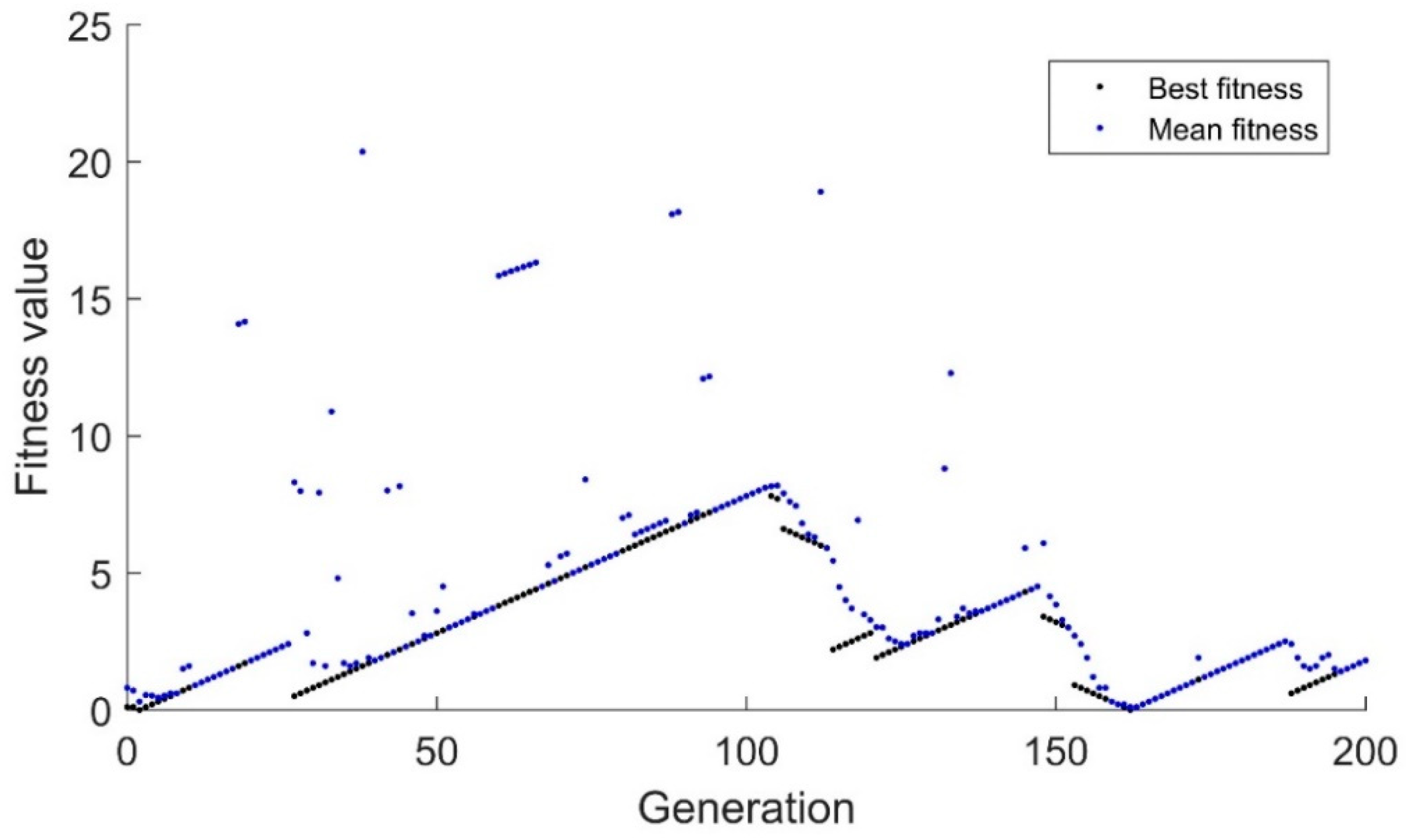
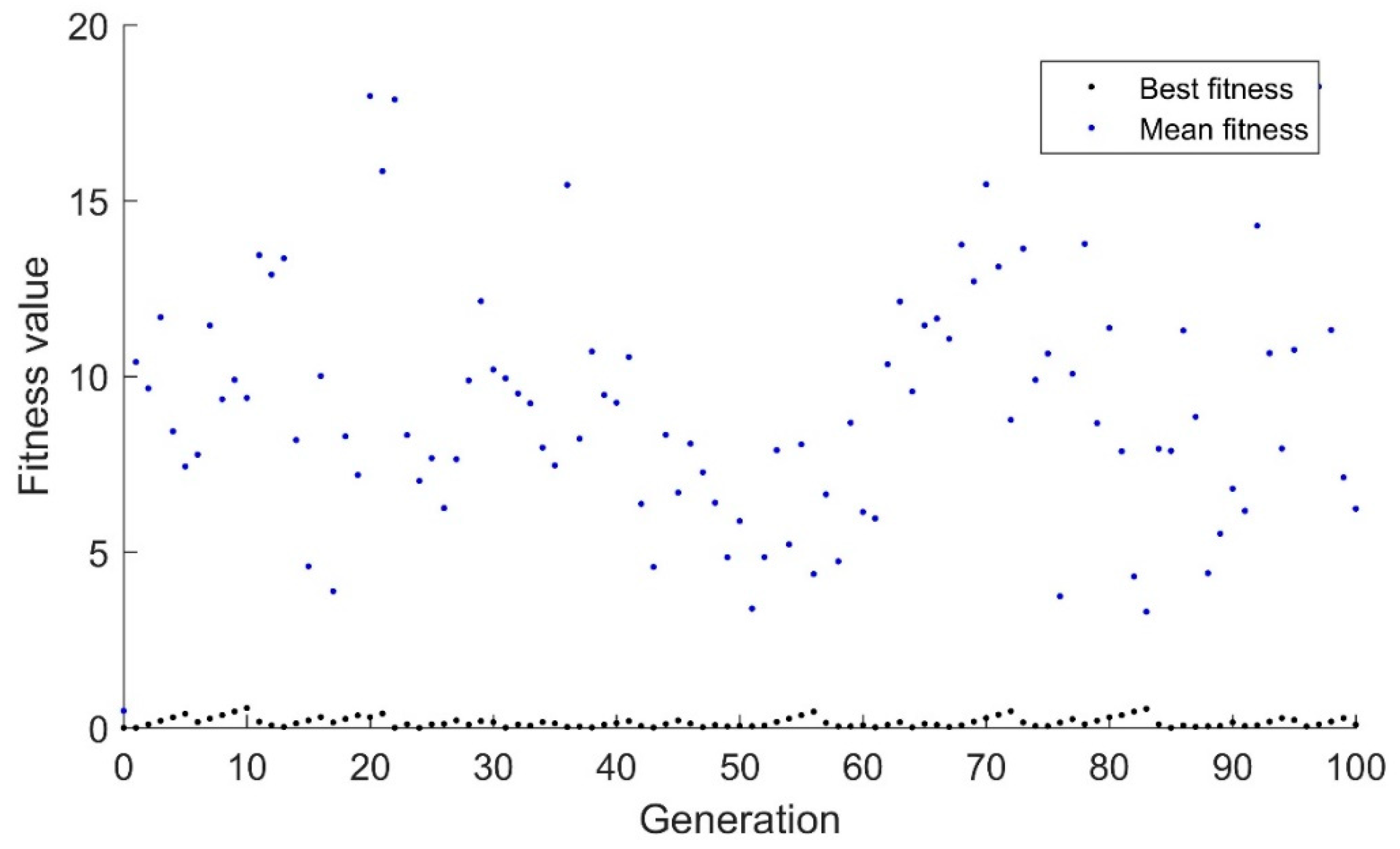
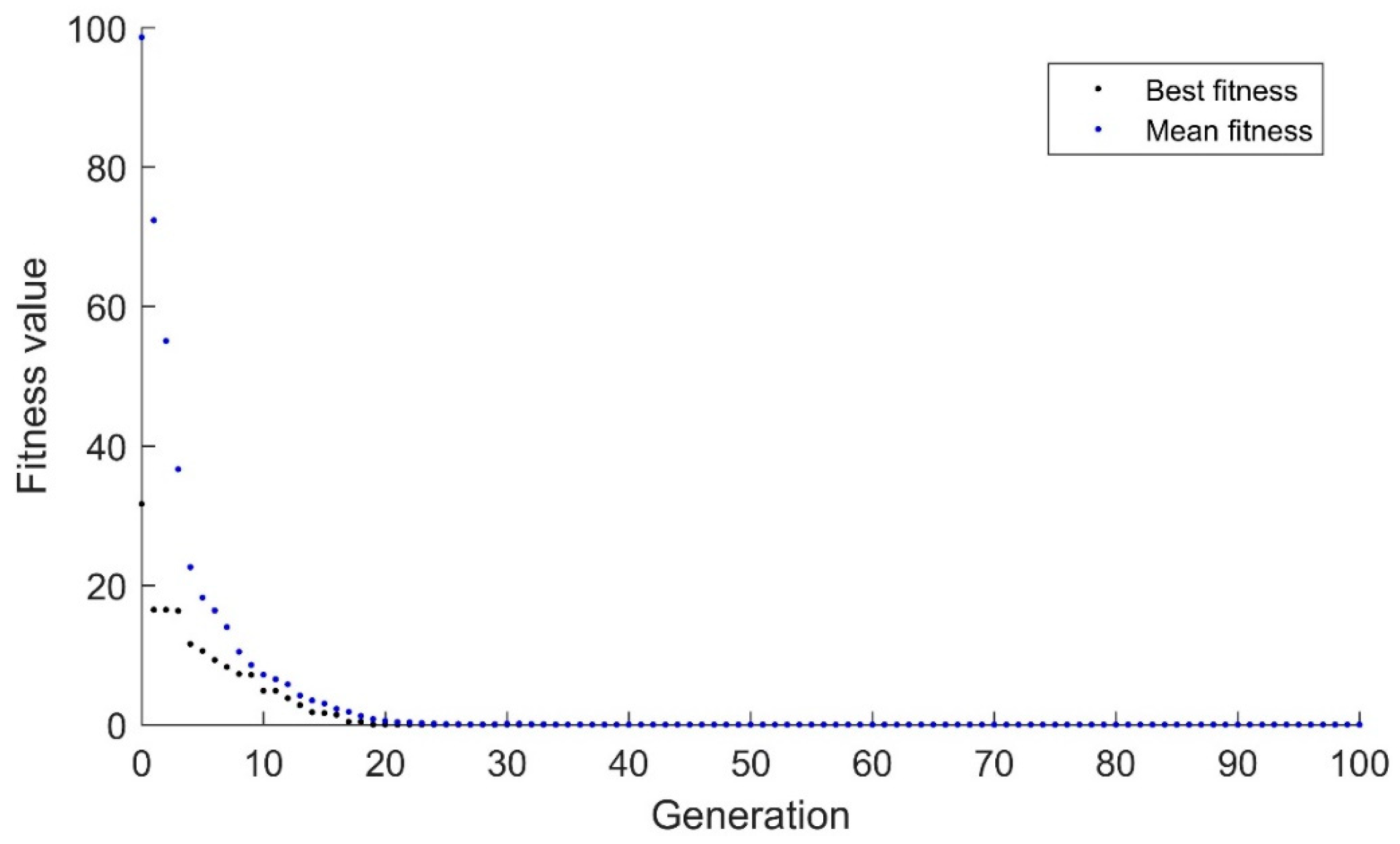
The binary genetic algorithm’s performance with the drifting goal is shown in Figure 1. The black dots represent the fitness of the best candidate while the blue dots represent the average fitness of all individuals in the population. As can be expected, since the algorithm uses a binary representation, only whole numbers are used, so the algorithm has a strong tendency for the best candidate to steadily increase or decrease in fitness. Additionally, since the binary algorithm relies heavily on mutation once convergence has been achieved, it is extremely difficult to adapt to minor changes. The mutation rate was set to a typical 1% for a 10-candidate population. This means that for every 10 generations, one mutation would be expected. Generations 95–103 have best fitness values and mean fitness values that are equal. This indicates that the algorithm has extremely limited diversity. This is a major point of concern because the algorithm has essentially converged despite being 8 units away from the target.

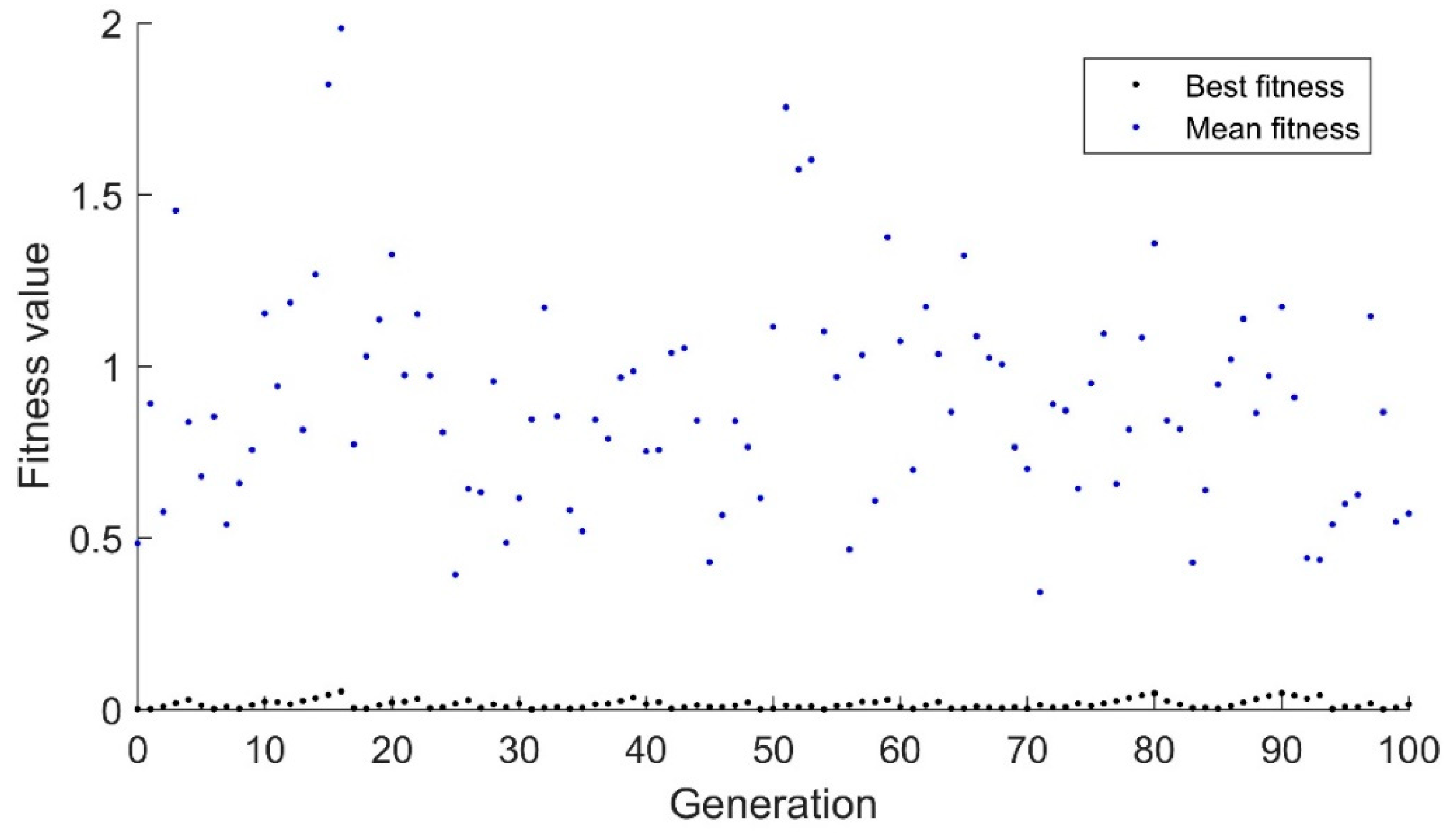
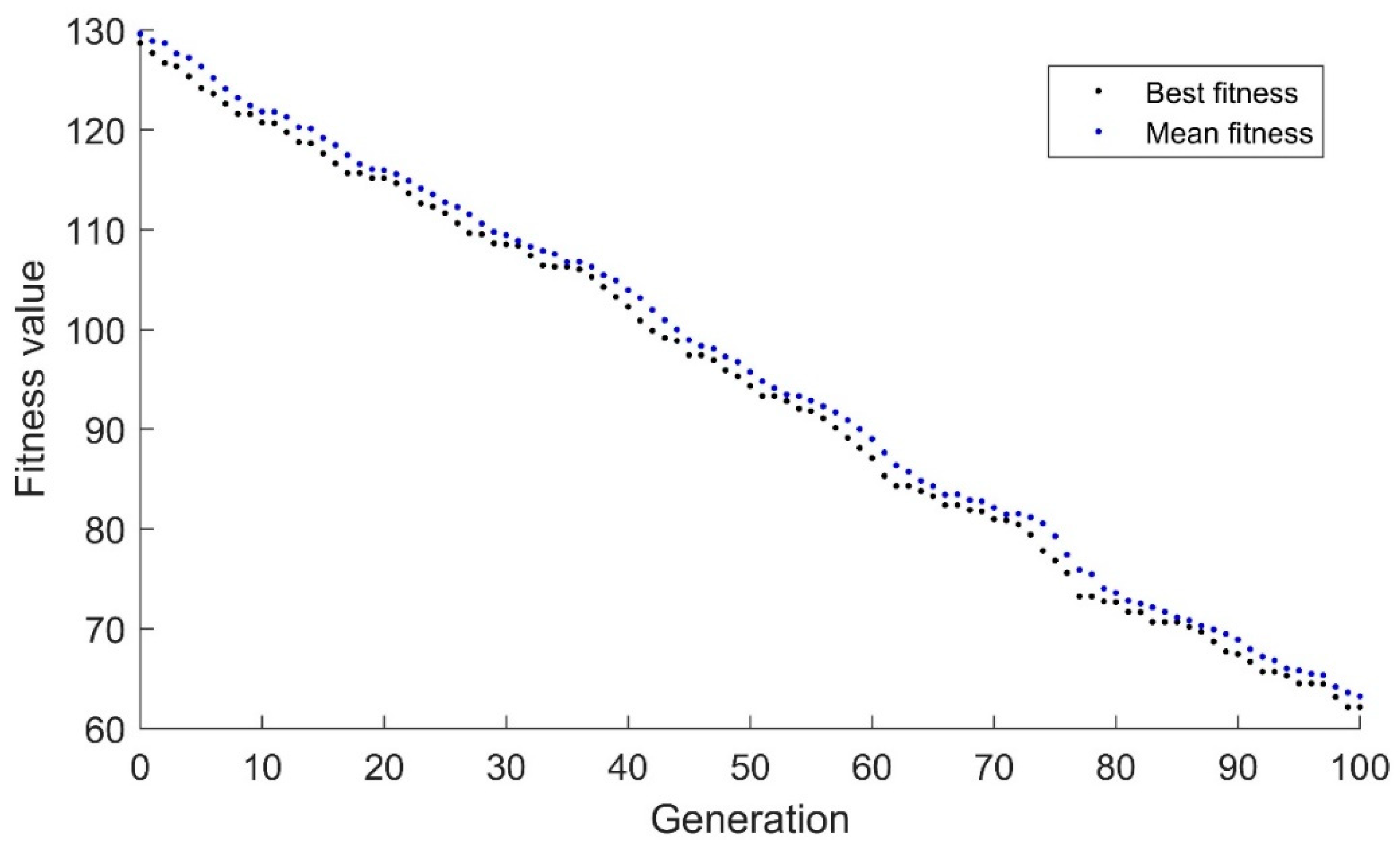
Figure 2 and Figure 3 demonstrate the response of the real-valued genetic algorithm to the same scenario. Again, mutation is the primary avenue for the algorithm to track the drifting goal with a mutation rate of 1%. However, in this application, the mutation is done via adding a normally distributed random variable to the child which has a mean of zero. In Figure 2, the standard deviation of the random variable is 0.01, while in Figure 3 the standard deviation of the random variable is 0.1. As can be seen, this algorithm does a much better job of tracking the drifting target than the binary algorithm. While the binary algorithm rarely had the best fitness below 1.5, the mean fitness of the real valued algorithm rarely has a mean fitness greater than 1.5 for Figure 2. In Figure 3, the mean stays high, but the best value stays below 1.

While Figure 1, Figure 2 and Figure 3 seem to indicate that the real-valued genetic algorithm is clearly superior to the binary genetic algorithm for this application, this depends highly on the way the algorithm is tuned and the type of application. Figure 4, Figure 5 and Figure 6 demonstrate the challenges associated with this. In these figures, the goal suddenly changes from 83 to −47 after the algorithm has begun to converge.

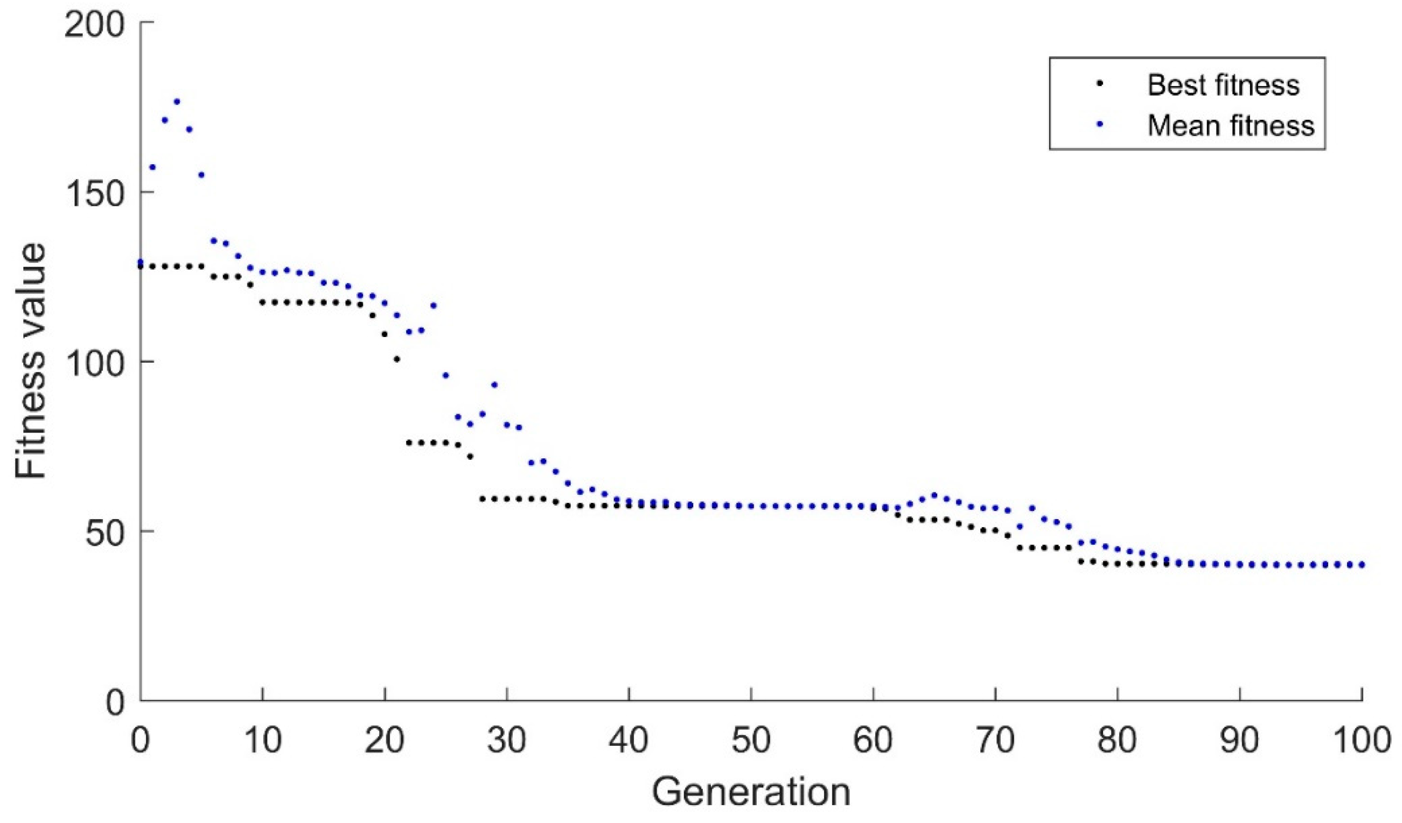
Figure 4 demonstrates the response of the binary genetic algorithm over the first 100 generations. As can been seen, the algorithm initially moves the mean toward the best individual, but the best individual takes a significant number of iterations to move closer to the target value. This algorithm finds the new optimum value at candidate 185 in this run. This example is generally nonrepeatable as the random mutations can cause the right mutation at any time. During 5 runs of this trial, the maximum was 273 generations while the minimum was 41.

The real-valued genetic algorithm that showed significant improvement in the drifting goal situation has an extremely hard time finding the optimum in the suddenly changing environment. In Figure 5, the algorithm can be seen to be slowly drifting toward the optimum value. Because the randomness is tightly constrained by the small standard deviation, 0.01, the algorithm cannot make sudden changes. This algorithm consistently takes ~200 generations to converge. 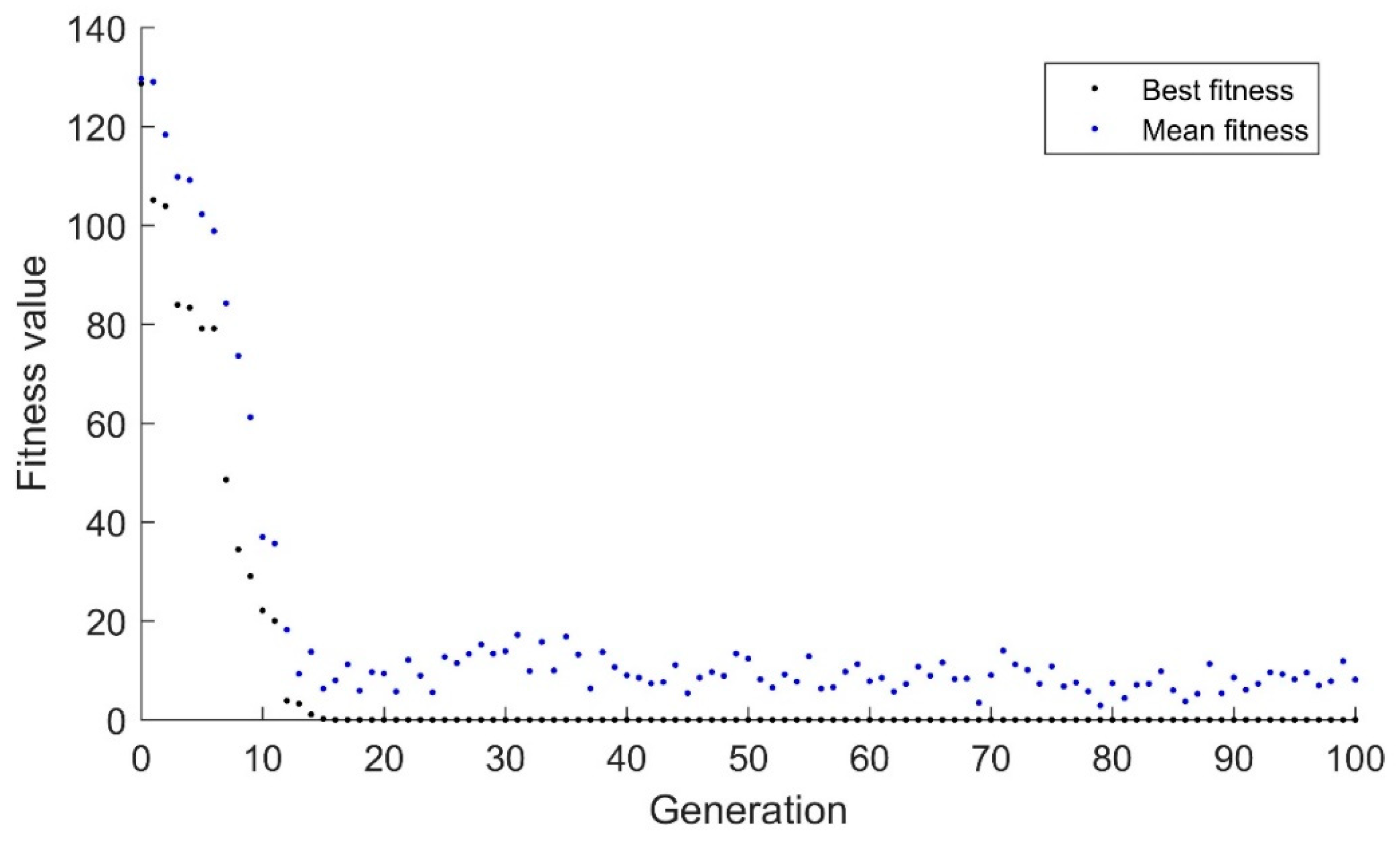In Figure 6, the increased standard deviation of 0.1 allows the algorithm to converge more quickly. However, it should be noted that the algorithm still tends to drift toward the goal. While this is likely reasonable in this application, if the goal changed from 830 to −470 instead of 83 to −47, the response would be like that of Figure 5 in the current range.

As stated previously, migration can augment mutation to increase diversity. Figure 7 demonstrates this effect. The population and mutation mechanics used in Figure 5 were implemented in Figure 7. However, when the sudden change in goal was detected, random candidates were added to the algorithm comprising 40% of the population. Overall, the algorithm finds the solution a little slower than the algorithm in Figure 6, taking 19 generations to arrive at an approximate solution compared to 16 previously. It has a much better mean fitness at the end of the algorithm, however. This means that the algorithm has more data points near the optimum at the end of the algorithm to get better resolution when converging. The algorithm converges to a much narrower band than in the Figure 4 through 6. In Figure 6, the best solution has an error of 2.66 × 10⁴ while in Figure 7 and the solution has an error of 1.22 × 10⁸. This is a significant improvement between the two.

As these figures indicate, there genetic algorithm often requires tuning to ensure proper results. In a fault-tolerant control problem, there may be insufficient information to tune the algorithm beforehand. As such, the genetic algorithms need major modifications to work in these environments. They also have a strong tendency to be drawn into local optima due to hill-climbing mechanics or produce inexact solutions due to limited resolution at the end of the algorithm. Migration holds the key to allowing the genetic algorithm to be able to leave local optima while still generating enough resolution during convergence. The AIS accomplishes this while also allowing memory to be included in the algorithm.

2.3. The Artificial Immune System

Genetic algorithms have been used for fault-tolerant control, though they have only been applicable recently [38]. AIS have been used to a limited extent in fault-tolerant control [39]. However, both have not seen widespread adoption. This is primarily due to the computational complexity of the algorithms. For basic problems, such as in [38,39], the control schemes are simple, and the algorithms have shown good results. However, the algorithms generally only use offline computation. As processor speeds increase and cloud computing becomes more available, these computations can be done in less time and can possibly be done near real time. The AIS focuses on integrating the principles of the biological immune system into the genetic algorithm.

In the natural immune system [40], plasma B cells attempt to neutralize contagions when an infection occurs. When the plasma B cells cannot respond well, memory B cells are activated that show a good response to a portion or the whole of the infection. When activated, these memory B cells generate many clones that travel to the infection site. During the cloning process, the new B cells undergo somatic hypermutation, allowing many variants of the memory B cells to flood the infection site. Somatic hypermutation is a transformation process that incorporates gene segments from the environment into the individuals. Assuming these new cells are fitter than the plasma B cells, they will replace cells in the plasma B cell population. From here, standard genetics mechanics continue in the plasma B cells while new clones are continually brought in if the response at the infection site is not as quick as desired. When the plasma B cells have discovered a solution to the infection, the solution is then stored as a new permanent member of the memory B cell population. This guarantees immunity to the infection if it is encountered again because the solution to the infection can be brought into the plasma population immediately.

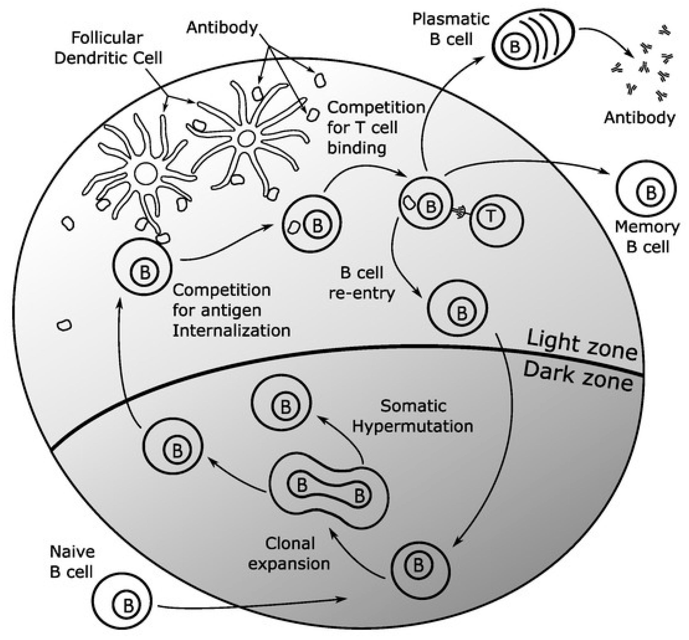
The approach in this paper will be a simplified version of the vertebral immune system. These models can add increased detail and complexity to provide improved performance. This increased detail can be applied as desired, but it is not required. For example, Figure 8 demonstrates a slightly more detailed version discussed as a germinal center [41]. The memory population mechanics discussed above all take place in the germinal center. The plasma population is represented in the diagram as the plasmatic B bells. The B cell in the memory population is shown at the bottom of the germinal center, where it undergoes clonal selection and somatic hypermutation. Before the B cells have a chance to enter the plasma population or get stored in the permanent memory population, this implementation adds additional competitive processes. The competition for targeted mutations by the follicular dendritic cells and the competition to be added to the plasma or permanent memory population through T cell binding increase the performance of the B cells that enter the population. These additional mechanics can shorten the response time of the AIS but are not required.

The AIS field is extremely active in terms of both applications and research [42,43]. Algorithm variants are produced frequently [42], including negative selection [44,45], immune networks [46], clonal selection [41,47,48], danger theory [49], dendritic cell algorithms [50], other models, or hybridized approaches. Of these, the most active in recently studies are clonal selection, negative selection, danger theory, and immune networks [51]. Immune networks are especially common as they are well suited to distributed or cloud computing. This paper focuses on the base clonal selection AIS introduced by de Castro and Von Zuben [48].

The AIS starts with a plasma population that is similar to the genetic algorithm population. In most applications, this needs to be done as a real-valued genetic algorithm. When the infection occurs, this plasma population attempts to fight it. For fault-tolerant control, this infection can represent an actuator that is not behaving as expected. The AIS will attempt to find a way to identify or compensate for this error depending on the needs of the application.

The plasma population follows the standard mechanics discussed in previous sections. Typically, it uses random individuals, plus some nonrandom, premeditated individuals. The premeditated individuals come from a databank of solutions to potential infections that could occur. For fault-tolerant control methods, these nonrandom individuals are solutions to known faults. If an actuator is known to be “finnicky”, an individual in the plasma population can be generated that is a potential compensation for that actuator’s finnicky behavior. If one of these individuals correctly compensates for the fault, the algorithm can respond immediately.

The randomly generated individuals are split into purely random individuals and random individuals that have minor traits from the databank added to them. These individuals allow the algorithm to get individuals “seeded” near potential solutions and minimize the computational time required to generate a feasible solution if the initial guesses are close, but not accurate.

After initialization, the plasma population uses elitism, crossover, and mutation as is standard in the typical genetic algorithm. However, it has an abnormally high level of migration, typically ~30% [52]. These migrants are not random individuals. Instead, they are generated as potential solutions based on the information in the databank. In Figure 8, the cells that survive competition for T cell binding and enter the plasmatic B cell population are the migrants.

The databank itself is stored in the dark zone of Figure 8. It is split into two parts: the memory population and the gene library. The memory population stores the individuals that show the best response to assorted known infections. These individuals are static and do not change over time. These individuals can be generated a priori based on experience with the system, can be generated through testing, or can be generated while the algorithm is running. This parallels the biological immune system where viable ways to combat an infection are inherited from parents, can be provided through inoculation, or can be developed after successfully fending off an infection. Typically, the memory population also includes randomized individuals. These often comprise half of the memory population or more. They exist to give the algorithm a starting point outside the known region in case a new, unexpected, issue arises that was completely foreign to previous experience. Most applications reset these random individuals every iteration to increase the likelihood that a random individual will be generated closer to the global optimum than any existing individual. This increases the available diversity without affecting the plasma population because these individuals stay separate from the plasma population unless they are good enough to be selected to be migrated over.

The other part of the databank is the gene library. It stores the different characteristics of the memory population. This allows variants of the memory population to be made quickly by adding these traits to existing individuals. The memory population has a slightly higher tendency toward randomization than the memory population because it is adding a supplemental mechanic for mutation. To prevent the mutation from being too controlled, random elements are added to the gene library to ensure the genetic diversity of the system is not compromised. The gene library can be populated through entirely random gene segments or a combination of random and nonrandom segments.

Clonal selection focuses on the somatic hypermutation that occurs during the cloning process. The memory candidates that produce the best response to the infection are determined by their performance according to the fitness function. Selection is usually determined by using the same selection process as the genetic algorithm operating on the plasma population.

Once the clones are generated, random elements from the gene library are added into the new clones at an extremely high rate. These rates can be upwards of 90–100%. Because the clones are added to the plasma population regularly, the high mutation rates prevent the system from becoming too homogenous. The mutated clones are then added directly to the plasma population. This process repeats every generation until a solution is produced.

There is some memory updating that must take place at this point. As the plasma population’s response to infection improves, the best individual in the plasma population is added to the memory population. If the fitness of memory population is constant or stays within some preset bounds, the algorithm assumes that the system is operating on the same infection. Since the same infection is being addressed, the algorithm updates a single individual in the memory population. The traits that define this new member of the memory population are extracted and added to the gene library.

If the fitness of the memory population leaves the acceptable bounds, then a new individual is added to the memory population, which will store the best candidate for the new fault. The best candidate for the previous fault is effectively frozen and will stay in the memory population in case the old fault occurs again. This can naturally lead to a major memory leak if not managed properly. This memory management is done on a per-application basis.

Applications of Artificial Immune Systems to Fault-tolerant Control

The artificial immune system can be implemented in several different methods for fault-tolerant control. Due it its inherent memory and learning attributes, the AIS can augment and overcome the limitations of other FTC methods. In the example provided in Section 3, the AIS is used for model reference adaptive control and multiple model control. This is one of the simplest applications for the AIS in FTC.

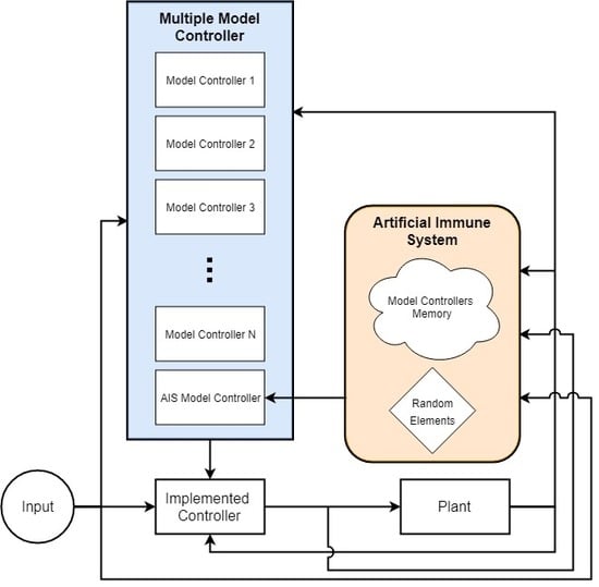
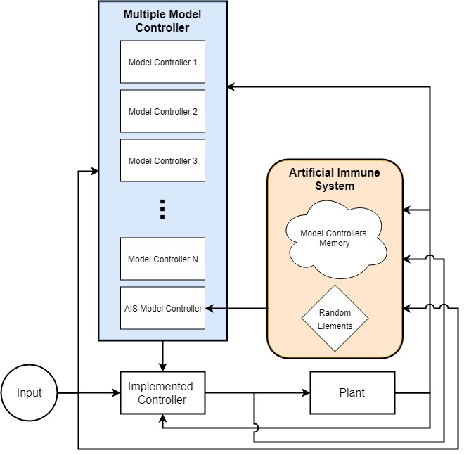
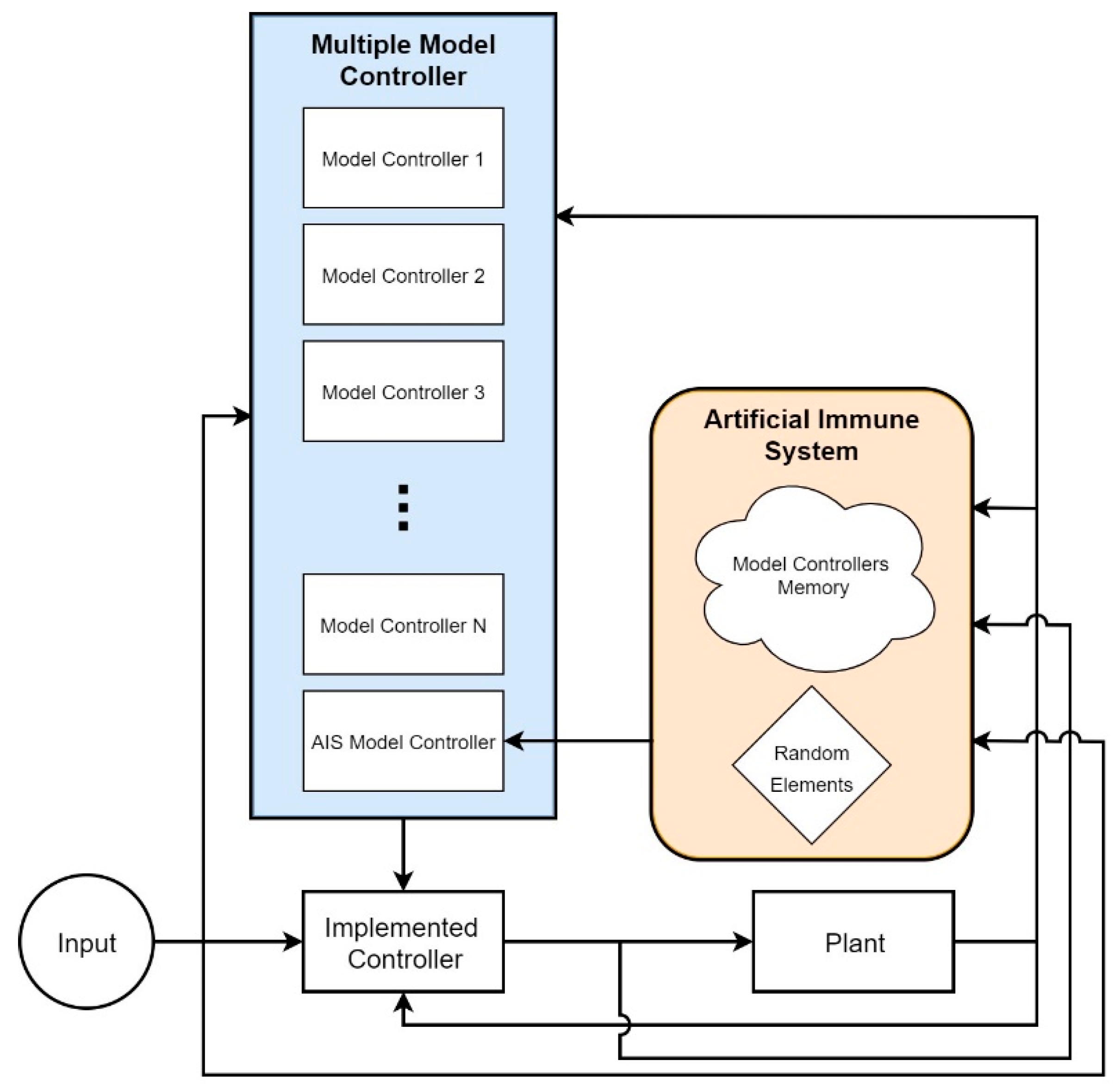
The introduction mentioned that the multiple model controller incorporated a priori information very well but had a limited range of solutions. If the fault was in the a priori information, compensation was quick and accurate. If it was not included, it is extremely unlikely to be compensated for sufficiently. An AIS can be incorporated into a multiple model control scheme by treating the controllers as individuals in the population. Thus, the controllers can be combined, reconfigured, and mutated to generate new models outside the original a priori set. An example of this can be seen in Figure 9. This allows the system to leverage the advantages of the original MM controller, including calculation speed, while mitigating its limitations when the fault is outside the faults predicted ahead of time. This implementation also mitigates the limitations of the AIS, namely its long computation times before convergence. The MM controller can act at a different speed than the AIS, providing some initial improvement immediately upon which the AIS can improve with each generation. Alternately, the MM controller portion could be absorbed directly into the AIS. In that case, the AIS would not only generate a controller, but also select the controller to be used. It would lose some response time as it would only be able to change controllers at the end of each generation.

These are options for implementing the AIS with the MM controller but should not be considered all encompassing. Regardless of the implementation mechanics, once the compensating controller has been determined, it is stored in memory and added to the a priori set of controllers. This ability to store solutions that had success in the past is what is critical in providing immunity. In FTC, this provides immunity to similar faults in the future. For swarm or distributed systems, this can also improve the performance of the group as it learns from the faults of the individuals. Essentially, the swarm develops immunity to a fault as soon as a single individual can overcome it.

The sliding mode and gain scheduling controllers can also benefit from the AIS. The AIS can be used to provide additional FTC capabilities when the system drifts outside the acceptable boundaries of the controller, similar to mechanisms that switch between active and passive compensation [5]. However instead of switching to a different precomputed controller or control scheme, the AIS could be used to choose between several different precomputed controllers, modify existing controllers, generate new controllers, or reschedule gains to improve performance. For the model predictive controller, when a fault occurs that is outside the preprogrammed realm, the AIS can perform additional compensation for sudden changes and nonlinear term injections by generating potential solutions until the controller’s functionality can be restored. These avenues allow the existing control scheme to function where it is designed to operate best, while expanding the operations when outside the existing conditions. The use of the AIS in these areas will need extensive study before any potential improvement claims can be verified.

3. Example Implementation of an Artificial Immune System

To demonstrate how an AIS can be implemented for fault-tolerant control, an example was built in MATLAB. For simplicity in the setup, the Optimization Toolbox was used to test many of the functions required. MATLAB’s Optimization Toolbox contains a customizable genetic algorithm function that can be used directly, or through a GUI. The function allows the user to define any necessary function for selection, crossover, mutation, and migration as well as optional functions to be called after each generation. Since the plasma population is managed through a real-valued genetic algorithm, it is highly advisable to ensure all custom functions operate as expected by using the Optimization Toolbox’s built-in functions.

Eventually, however, the AIS will need to be generated independently of the toolbox. For this example, consider a four-wheeled rover controlled by 6 actuators: 4 in-hub drive motors and 2 steering motors, one for the front wheels and one for the rear wheels. The vehicle dynamics are beyond the scope of this paper. Suffice it to say that the equations of motion are highly complex and nonlinear since they do not necessarily follow the standard bicycle model. The rover was simulated in MATLAB to avoid the issues that arise in physical testing, such as sensor noise. The system is overactuated to ensure the system retains full mobility after a failure. While nothing prevents the AIS from being applied to just-actuated or underactuated systems, the target system here is designed to still be functional if an actuator experiences complete failure. In other instances, the system’s limited maneuvering envelope would need to be compensated for through additional mechanics.

The algorithm will attempt to compensate for faults in the actuators by considering them to be changes in the effective control signal. That is, if a motor is 50% effective, the control signal would need to be doubled to generate the same output. This will essentially mean the control signal can be represented by a six-entry column vector (u) that gets multiplied by a 6 × 6 matrix (B). When all actuators are operating normally, the B matrix is an identity matrix as shown in Equation (8).

$$\mathbf{u}\prime =\mathbf{B}\times \mathbf{u}= \left[\begin{array}{cccccc}1& 0& 0& 0& 0& 0\\ 0& 1& 0& 0& 0& 0\\ 0& 0& 1& 0& 0& 0\\ 0& 0& 0& 1& 0& 0\\ 0& 0& 0& 0& 1& 0\\ 0& 0& 0& 0& 0& 1\end{array}\right]\ast \left[\begin{array}{c}{\mathrm{u}}_1\\ {\mathrm{u}}_2\\ {\mathrm{u}}_3\\ {\mathrm{u}}_4\\ {\mathrm{u}}_5\\ {\mathrm{u}}_6\end{array}\right].$$

(8)

This matrix can allow for full actuator failures, partial actuator failures, actuators influencing each other, and so forth. These are not all possible effects, but they represent a large swath of possible failures. Each entry in the B matrix will have a maximum allowable value of 2.55 and a minimum value of −1. This was selected based on the limitations of the hardware that this algorithm could be implemented on in future work. These numerical limitations are highly application dependent.

The number of effects that the algorithm can account for can be increased by incorporating these issues as additional control effects. This has been demonstrated previously [53]. For this work, a demonstration of the abilities of the AIS, only the B matrix will be used. It should also be noted that this paper will address the use of the AIS to identify the fault so that it could be appropriately compensated by a controller. The mechanics of this compensation is beyond the scope of this work. As such, it is assumed that a simple pseudo-inverse can be used to generate a compensating matrix to counter the effects included in the B matrix.

The fault that the AIS will be attempting to solve is shown in Equation (9).

$$\mathbf{B}= \left[\begin{array}{cccccc}0.9& 0& 0& 0& 0& 0\\ 0& 0.5& 0& 0& 0& 0\\ 0& 0& 1& 0& 0& 0\\ 0& 0& 0& 1& 0& 0\\ 0& 0& 0& 0& 1& 0\\ 0& 0& 0& 0& 0& 1\end{array}\right].$$

(9)

This corresponds to a 90% fault in actuator one and a 50% fault in actuator two. The front-left motor and front-right motor are actuators one and two respectively.

For the AIS implementation, an individual will consist of 36 real-valued variables that represent the entries in the B matrix. Known faults will be included in the memory population by generating the individuals that represent those faults. For example, any motor could be completely non-responsive. The B matrix representing these faults will have one value on the diagonal set to zero instead of one. For partially effective motors, the entries on the diagonal can be set to a value between zero and one.

The fitness of the candidates is calculated through the location discrepancy between the trajectory predicted by a given individual and the trajectory travelled by the faulted vehicle, the difference in shape between the two trajectories, and the number of entries in the matrix that differ from the identity matrix. The location error is determined by subtracting the location of each data point along the trajectory. The shape error is determined through a Procrustes analysis. Including the number of entities different from the identity matrix in the fitness function minimizes the complexity of the matrix. Each of these factors has a weighting factor which is determined through testing.

For the purpose of this example, the initial population and memory population were not given useful a priori information and were intentionally lacking candidates that had any noticeable changes in the first two diagonal entries in the B matrix. This was done to make sure the algorithm has a sufficiently difficult task to work on. Other than this constraint, the individuals in the initial plasma and memory population were generated randomly save for the first individual in the memory population. This individual will represent the unfaulted system. The plasma and memory populations will both have 100 individuals in them. Unfortunately, this is less than the recommended number, but this number of candidates was chosen to make the calculations finish in a reasonable timeframe. The gene library will have 100 random elements and 100 elements that correspond to portions of the memory population. The random elements were generated by creating elements of randomized length and values that could be added directly to any individual.

Once all these portions of the algorithm are initialized, the fitness of all individuals in the memory and plasma populations is evaluated. If the fitness is outside the acceptable threshold, then the individuals in the plasma population are ranked by their fitness. The top 5 individuals of the plasma population are passed on to the child generation directly, corresponding to a 5% elitism rate.

The selection process to generate the crossover children was implemented as stochastic uniform selection. In total, 130 individuals were selected to generate 65 children. These 65 new children correspond to a 65% crossover rate. The 130 individuals were randomly reordered and consecutive pairs were chosen for reproduction through crossover.

Crossover was performed through a uniform crossover coefficient applied on the entire candidate. The B matrix of the first individual paired for reproduction was subtracted from the B matrix of the second individual. The difference between these two was then multiplied by a random coefficient between 0.5 and 1.5 before being added to the first individual.

Mutation is implemented by randomly selecting 13 individuals from the children produced by crossover, corresponding to a 20% mutation rate. A random entry in the B matrix is selected and changed to a value between the maximum and minimum allowable values, 2.55 and −1, respectively.

The remaining 30 individuals in the child population are generated through the migration of clones from the memory population. The cloning process was instigated by ranking the individuals in the memory population by their fitness. Stochastic uniform selection was then used to select the best individuals from the memory population for cloning. Since 30 individuals were to be added to the child population, 30 individuals were selected from the memory population to be cloned. Random elements from the gene library were added to 90% of the clones. There is some debate about whether the memory individual selection should be done over the entire population, over a high-performing subpopulation, or if only the single best individual should be used. These individuals are then added to the child population directly.

The memory population is updated before the children are allowed to mature into a new parent population. A new blank candidate is added to the memory population as the 101st individual. This individual will be used to store the eventual solution to the problem at hand. The individual with the best fitness from the plasma and memory population is stored in the blank candidate as the best solution to date. The gene library has an entry added to it as well. This 201st gene library segment will always store the traits that define the best solution to date.

Because this example did not have any useful a priori data stored in the memory population or the gene library, the randomly generated individuals and gene library segments are regenerated. That is, individuals 1 through 100 in the memory population were replaced by randomly generated individuals. The 101st individual was not changed. Gene library segments 2–100 were recalculated according to the traits that defined the first hundred new memory individuals. Gene library segments 101 through 200 were replaced by randomly generated segments. The 201st segment was not changed.

After the memory update is complete, the child population is matured by moving them into the plasma population, replacing the previous generation. The fitness of the new plasma population is calculated. If any value is below the threshold indicating a solution has been found, the algorithm is terminated and the plasma individual with the lowest fitness is returned as the solution to the problem. If this does not occur, then selection, crossover, and mutation are implemented in the plasma population as explained previously.

However, at the end of this phase, the memory update must be performed differently. Firstly, when the fitness of the memory population is evaluated, the fitness of all nonrandom individuals in the population is evaluated compared to their previous values. In this stage of this application, the 1st and 101st individuals are nonrandom. If the fitness values change substantially, then a new fault is considered to have occurred. In that case, a 102nd individual is created in the memory population and a 202nd segment is added to the gene library. Otherwise, the algorithm continues through clonal selection as discussed previously.

Assuming the fault state has not changed, the 101st memory candidate is updated with the best performing individual from the plasma population. The 201st gene library segment is updated based on this individual.

This process continues until the threshold indicating a solution has been found, the algorithm converges, or a limit has been reached—such as a maximum number of generations or maximum computation time.

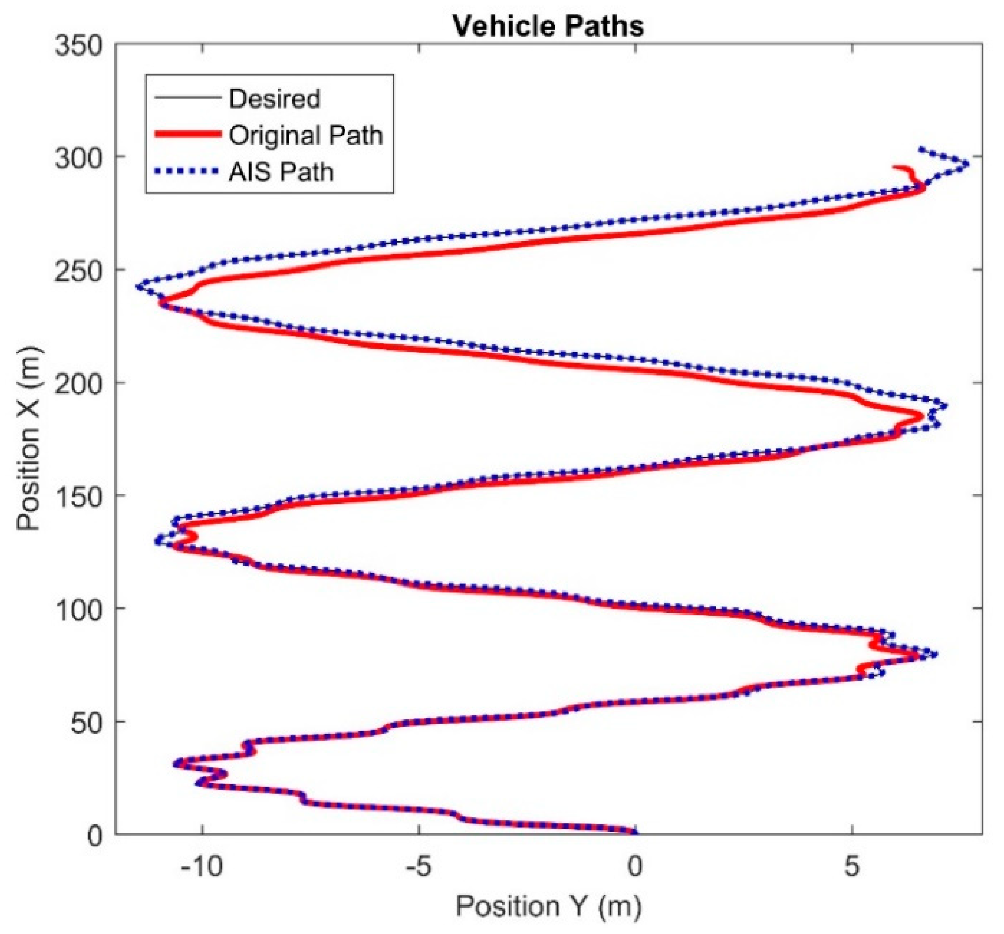
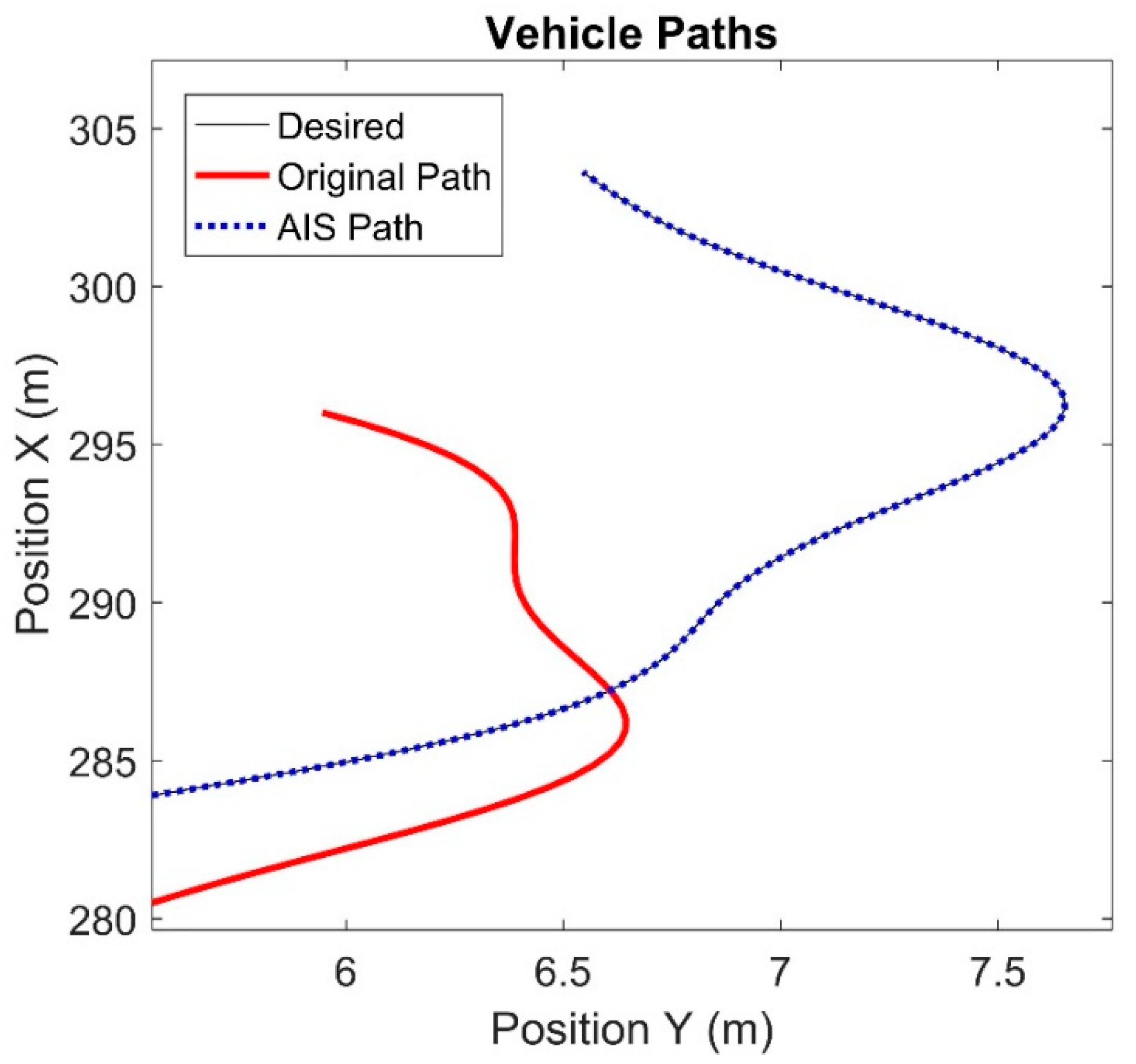
The results of this algorithm are shown in Figure 10, Figure 11 and Figure 12. Figure 10 shows the trajectory of the vehicle. The control signals passed to the system were cyclical, generating the S-curved path shown. The black line represents the desired path of the vehicle. This is the path the vehicle would take if no actuator faults occurred. The red trajectory shows the path that the vehicle travelled when the actuators were faulted. This is the original path the vehicle followed before any compensation was performed. Using this data, the AIS ran until termination. A compensating controller was generated from the output of the AIS and the simulation was rerun with the same signals being fed to the compensating controller, which then sent commands to the vehicle with the faulted actuators. The blue dotted line indicates the path that the vehicle travels when the compensating controller is sending commands to the vehicle.

Figure 11 shows an enlarged version of Figure 10, focusing on the final moments of the vehicle. The black line is nearly indistinguishable from the blue dots, indicating that the vehicle is following the trajectory extremely closely. The location error between the desired path and the compensated path oscillates due to the variation in the control signal and steadily increases. However, it is never more than 0.1 meters. This is significant as the vehicle travels over 300 meters.

Unfortunately, the solution is not exact. The AIS ran for 46 generations and evaluated 4600 individuals in the plasma population. The algorithm took 1 hour and 48 min to complete on a Lenovo T530 laptop with a quad-core Intel i7-3720QM processor running at 2.60 GHz with 16 GB of RAM. Due to the length of the trial required, the threshold for acceptable solutions was set low enough to permit inexact solutions. In part, this was a design choice. Fault-tolerant control needs to be able to safely control the system, not optimally control the system. If the algorithm continued, a better solution could have been obtained, but the performance of the system with the inexact solution would be acceptable for most applications.

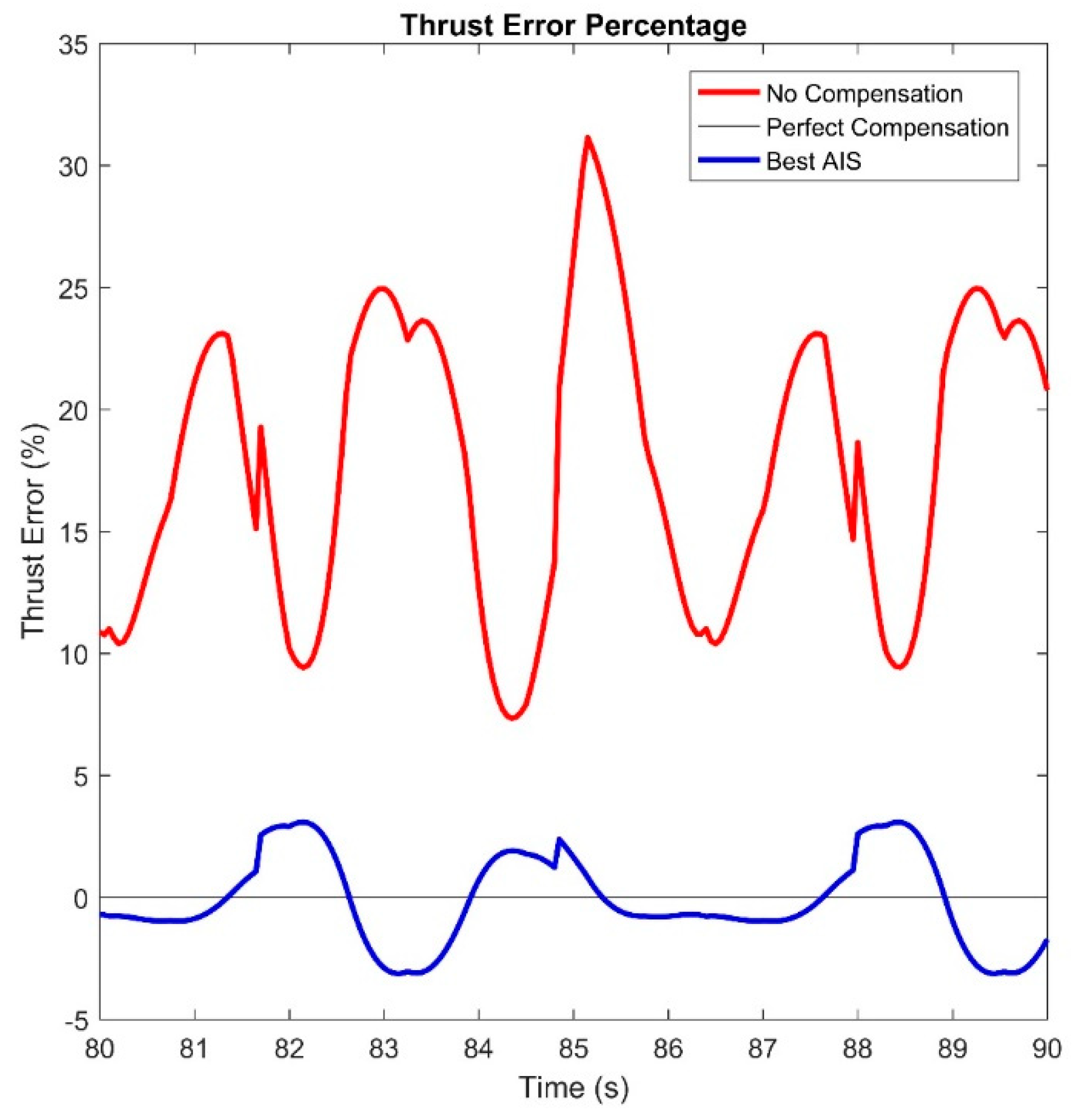
Because the solution is inexact, the algorithm neither follows the correct trajectory perfectly, but also has an error in thrust. The thrust error is shown in Figure 12. This is calculated as the difference between the forward thrust provided by the wheels and the thrust the desired system would provide. As can be seen, system provides significantly better thrust than the original system, but it is noticeably incorrect. Because the error oscillates, the overall vehicle follows an accurate path overall as the times the thrust is high and low balance over time.

One of the major advantages of the AIS is the ability to learn from previously encountered faults and neutralized them quickly when they are encountered again. To demonstrate this, at the end of the experiment shown above, the fault was removed. The AIS identified that the fault state changed and identified the unfaulted candidate—the one stored as the first individual in the memory population—as the optimal solution. As a result, it returned this as the final solution immediately. When the fault was reintroduced, the previous solution—the one stored as the 101st individual in the memory population—was returned as the solution immediately. While this candidate was not optimal, it was within the performance threshold to be returned as an acceptable solution. A full generation was not required for these computations, indicating that time will not be a factor in compensating for these errors.

4. Conclusions

The AIS has begun to show promise for fault-tolerant control. They are still unreasonably slow when used on standard CPUs as indicated by the runtime of a little under two hours in the example above. Again, it should be noted that 100 individuals were used in the example despite the literature recommending 360 individuals, 10 for each variable to be solved for.

However, because the majority of the calculations within the AIS are not mutually dependent, the AIS can be highly parallelized. The only nonparallelizable calculations are relatively simple, such as the selection and fitness ranking steps. This allows the AIS to be run much faster on distributed or cloud computing setups. Depending on the complexity of the parallelizable functions, these could even be run on GPUs or FPGAs where many computational threads are available.

With improvements to the computational speeds available as well as improvements in the speed of the algorithms, the AIS could become a feasible alternative for real-time fault-tolerant control. Initially, these would need to be performed in low-speed environments, such as maritime shipping where stopping a modern cargo ship going full speed can take up to 20 min. In this application, the algorithm can be allowed much more time to determine a solution compared to a car which can take 5 seconds to stop safely at highway speeds.

Future work will involve trialing the algorithm in these environments, optimizing the algorithm for increased speed, and implementing the algorithm on higher-speed machines.