Article

Trajectory Tracking Control for Lane Change Maneuvers: A Differential Steering Approach for In-Wheel Motor-Driven Electric Vehicles
College of Automobile and Traffic Engineering, Nanjing Forestry University, Nanjing 210037, China
*
Author to whom correspondence should be addressed.
Actuators 2026, 15(4), 205; https://doi.org/10.3390/act15040205
Submission received: 12 February 2026 / Revised: 30 March 2026 / Accepted: 31 March 2026 / Published: 4 April 2026

Abstract

To ensure reliable lane change behavior in-wheel motor-driven electric vehicles (IWM-EVs) under steer-by-wire (SBW) failure, this paper presents an integrated lateral–longitudinal lane change control strategy based on differential steering. The control framework and relevant models are first established. An upper-layer model predictive control (MPC) controller is then designed to simultaneously achieve lateral path tracking and longitudinal speed regulation, outputting the desired front-wheel steering angle and acceleration. Finally, a model-free adaptive control (MFAC)-based lower-layer lateral controller transforms the desired steering angle into differential driving torques for the front wheels, while a feedforward–feedback lower-layer longitudinal controller (incorporating drive/brake switching and PI control) computes the required driving torque or braking pressure. Co-simulation in Matlab/Simulink R2022b and CarSim R2020 reveals that the MPC controller designed in this study outperforms the LQR-PID controller, reducing the maximum absolute values of lateral error, heading error, front-wheel steering angle, yaw rate and sideslip angle by 42.9%, 50.0%, 7.8%, 2.8% and 10.3%. The proposed hierarchical control strategy outperforms the compared hierarchical controller, reducing the maximum absolute values of the lateral displacement error, heading error and yaw rate by 17.9%, 6.7%, and 33.3%. These results verify that the strategy can improve trajectory tracking accuracy and achieve basic differential steering functionality in specific scenarios.

1. Introduction

In-wheel motor-driven electric vehicles (IWM-EVs) offer independent torque control for each wheel and flexible control capabilities, thus supporting differential steering during steer-by-wire (SBW) system failure. Differential steering realizes vehicle steering through wheel speed difference control—characterized by quicker response and greater flexibility than traditional systems [1]—or specifically via torque difference between the left and right drive wheels [2,3].
For differential steering control, Peng et al. [4] verified yaw rate calculation accuracy using a back propagation neural network (BPNN) and matched it with an anti-saturation proportional-integral-derivative (PID) controller for torque distribution. Hu et al. [5] integrated it into a differential drive assistance steering system, stabilizing vehicle lateral dynamics with integral sliding mode control (SMC) and reducing sliding mode surface chattering via the adaptive super-twisting strategy. Chen et al. [6] proposed non-singular terminal SMC, realizing robust tracking of the desired front-wheel angle via differential steering, even with complete steering motor failure. These studies all demonstrate that differential steering effectively enables normal steering under failure.
Vehicle lane change, a key technology in autonomous driving, is crucial for ensuring safe, smooth and comfortable lane change maneuvers. Thus, numerous scholars have conducted extensive research on lane change trajectory planning and tracking [7,8,9]. Additionally, IWM-EVs eliminate traditional mechanical transmission systems, enabling independent torque control of the four drive wheels and offering high transmission efficiency as well as enhanced active safety [10,11]. Designing lane change control strategies for such vehicles has therefore become an urgent task.
To ensure safe and smooth lane changes for intelligent vehicles, lane change trajectories must satisfy vehicle kinematic, dynamic, and surrounding road environment constraints [12,13]. Zhang et al. [14] developed an improved A* trajectory planning algorithm, proposing a new heuristic function integrating distance and obstacle information to address the A* algorithm’s unsmooth trajectory issue. Zeng et al. [15] presented a trajectory planning scheme for autonomous vehicle lane change, which adopts B-spline for path generation and RRT as a supplementary method, and introduces a trajectory monitoring strategy to improve the robustness and safety of lane change in complex driving scenarios. Despite good planning performance, these methods have high computational loads and suit scenarios with numerous fixed obstacles [16]. Polynomial curves are widely used for lane change trajectory planning due to their simple structure, continuous curvature, and ease of constraint addition [17,18]. For instance, Ding et al. [19] utilized a fifth-degree polynomial curve, adjusting transition time and longitudinal displacement to plan trajectories meeting safety, timing, and comfort requirements.
Trajectory tracking is critical to ensuring vehicles follow the reference lane change trajectory, and balancing tracking accuracy and stability is core to controller design [20,21,22,23,24,25]. Carlucho et al. [26] proposed a multi-PID hybrid strategy by combining deep reinforcement learning with PID control, enhancing lateral control accuracy for complex scenarios. Kapania and Gerdes [27] developed a feedforward–feedback tracking controller to improve steering stability and reduce lateral position bias, yet it is inapplicable to variable-speed lane-changing vehicles. For intelligent vehicles, Huang et al. [28] presented an optimized model predictive control (MPC)-based lane change obstacle avoidance controller to address safety issues when avoiding obstacles on low-adhesion roads. Integrating road adhesion coefficients with obstacle avoidance path planning, their designed trajectory-tracking controller effectively enhances driving safety and stability.
For the trajectory tracking of IWM-EVs, Li et al. [11] designed a lateral path model predictive control (MPC) controller and a longitudinal velocity PID controller, verifying their performance via simulations. To address vehicle stability issues arising from lateral–longitudinal motion coupling under highly nonlinear tire conditions, Li et al. [29] proposed a coordinated lateral–longitudinal controller based on the LuGre combined anti-skid tire model. Sun et al. [30] developed a low-speed tracking controller using fuzzy proportional-integral (PI) control and an upper path tracking controller via optimal control; their improved coordinated controller balances tracking accuracy and driving stability across different speeds. Park H. et al. [31] presented a path tracking system for such vehicles, integrating optimal four-wheel torque allocation while considering speed, heading angle, and lateral position constraints.
In summary, the existing literature on IWM-EV lane change trajectory tracking mostly decouples lateral path and longitudinal speed control, relying on traditional steering or SBW. Research on differential steering for such trajectory tracking remains limited. Given the independent torque control of in-wheel motors, adjusting the torque difference between the left and right front wheels via a front-wheel differential steering system (FWDSS) can restore normal steering if the SBW fails. This study thus investigates lane change trajectory tracking for these vehicles using differential steering under SBW failure. The main contributions of this paper are as follows:
(1)
Using lateral and longitudinal error models, an MPC-based upper controller is developed to simultaneously track the lateral path and longitudinal speed, outputting the desired front-wheel steering angle and acceleration for trajectory following.
(2)
A model-free adaptive control (MFAC)-based lateral lower controller is designed for the front-wheel differential steering vehicle (FWDSV) to track the reference model’s sideslip angle and yaw rate, generating left/right front-wheel differential driving torques.
(3)
The longitudinal lower controller, incorporating a drive/brake switching strategy and a PI controller, converts the upper controller’s desired acceleration into the required driving torque or braking pressure for the IWM-EV’s longitudinal speed tracking.
The rest of this paper is organized as follows: Section 2 outlines the controller framework and introduces the relevant models; Section 3 details the controller design, including the upper controller and lateral/longitudinal lower controllers; Section 4 presents performance comparisons of the upper controller and the hierarchical controller; and Section 5 summarizes the whole paper and draws final conclusions.

2. Control Framework and Relevant Models

In this paper, a differential steering vehicle (DSV) is adopted as the research object. If the steer-by-wire (SBW) malfunctions due to the failure of the steering motor, the vehicle restores its normal steering capability with front-wheel differential steering, and, in this condition, it becomes rear-wheel drive. That is to say, the rear wheels provide longitudinal traction to propel the vehicle and the front wheels are decoupled from longitudinal traction; instead, the differential torque applied to them is exclusively used to generate lateral steering moments. This functional separation ensures no conflicts between longitudinal traction and lateral steering demands.
In this section, we will introduce the control framework, lane change trajectory planning model, trajectory tracking error model, reference model, inverse driving model, and inverse braking model.

2.1. Control Framework Definition

The controller framework is outlined in Figure 1. In the figure, a trajectory planning model is adopted to generate the reference lane change trajectory. The upper controller employs the MPC to enable the DSV to track the reference trajectory in real-time. The lower controller consists of two sub-controllers: lateral and longitudinal. The lateral lower controller adopts MFAC to regulate the yaw rate and sideslip angle of the DSV model to match the reference model under the given steering angle. The longitudinal lower controller determines the driving torque of the rear in-wheel motors or the braking pressure of the CarSim-based DSV model.
Figure 1. Overall hierarchical control framework and co-simulation interface between Matlab/Simulink R2022b and CarSim R2020, where discrete-time implementation is denoted by T s = 0.01 s. In this figure, blue solid arrows indicate signal flow, and color-coded boxes denote different functional modules of the hierarchical control framework. Relative variable definitions are listed in Table 1.
Actuators 15 00205 g001
Table 1. Related parameters of Figure 1.
Module NameSymbolDefinition
Trajectory Planning Model X t 0 , Y t 0 Initial longitudinal and lateral vehicle displacement
d f Longitudinal displacements after
the lane change manuever
w Lateral displacements after the lane
change manuever
t f Lane change completion time
X r e f k , X ˙ r e f k Longitudinal position and velocity of
reference trajectory at time step k
Y r e f k Lateral position of reference trajectory
at time step k
θ r e f k , κ r e f k Heading angle and reference curvature
at time step k
Upper Controller (MPC) δ f Front wheel steering angle
a d e s Desired longitudinal acceleration
Lateral Lower Controller ω d , β d Desired yaw rate and sideslip angle
ω , β Actual yaw rate and sideslip angle
T f r , T f l Driving torques of the left and right front wheels
M f l , M f r Actual output torque of the left and right
front in-wheel motor
Longitudinal Lower Controller e a Error between desired and actual
longitudinal accelerations
T t Required driving torque of the in-wheel motor
M r l , M r r Actual output torque of the left and right
rear in-wheel motor
P b d e s Desired brake pressure
DSV Model of CarSim a a c t Actual longitudinal acceleration
X k , Y k Longitudinal and lateral displacement of
vehicle CG at time step k
φ k , φ ˙ k Yaw angle and yaw rate of vehicle CG
at time step k
X ˙ k , Y ˙ k Longitudinal and lateral velocity of vehicle
CG at time step k

2.2. Lane Change Trajectory Planning Model

A fifth-degree polynomial curve is used to represent the lane change trajectory in the most prevalent two-lane situation. It is assumed that the vehicle’s positions before and after the lane change are on the centerline of the road. The schematic of the lane change trajectory is given in Figure 2, where X O Y is the global coordinate system, the coordinate origin O is the vehicle center of gravity (CG) position at the initial moment of lane change, the X axis and Y axis are the longitudinal and lateral directions of the vehicle body, and X r e f and Y r e f are the desired longitudinal and lateral positions of the vehicle’s CG, respectively.
The lane change trajectory defined by the fifth-degree polynomial curve is as follows:
X r e f t = a 0 + a 1 t + a 2 t 2 + a 3 t 3 + a 4 t 4 + a 5 t 5 Y r e f X = b 0 + b 1 X + b 2 X 2 + b 3 X 3 + b 4 X 4 + b 5 X 5 ,
where t is the time variable, and a 0 ~ a 5 and b 0 ~ b 5 are the constant coefficients.
The second equation in Equation (1) can be transformed into the following:
Y r e f t = Y r e f X r e f t Y ˙ r e f t = Y r e f X r e f t X ˙ r e f t Y ¨ r e f t = Y r e f X r e f t X ˙ r e f t 2 + Y r e f X r e f t X ¨ r e f t .
The heading angle θ r e f and curvature κ r e f of the reference trajectory are expressed as follows:
θ r e f t = arctan Y r e f X r e f t κ r e f t = Y r e f X r e f t / 1 + Y r e f X r e f t 2 3 / 2 .
In summary, the lane change trajectory in a two-lane scenario can be represented by Equations (1)–(3).

2.3. Trajectory Tracking Error Model

2.3.1. Lateral Trajectory Tracking Error Model

Here, the linear two-degree of freedom (2DOF) vehicle model shown in Figure 3 is used to describe the lateral trajectory tracking problem of an IWM-EV using the traditional steering method, where x o y is the vehicle coordinate system; the vehicle’s CG is selected as its origin o ; X , Y are the coordinates of the vehicle’s CG in the X O Y coordinate system; F y f and F y r are the lateral forces on the front and rear tires, respectively; and v r e f and θ r e f are the longitudinal velocity and heading angle of the reference point on the reference trajectory.
From Figure 3, the simplified model of the 2DOF vehicle can be expressed as follows:
v ˙ y = C f + C r m v x v y + a C f b C r m v x v x ω C f m δ f ω ˙ = a C f b C r I z v x v y + a 2 C f + b 2 C r I z v x ω a C f I z δ f ,
where m is the vehicle mass, I z is the vehicle yaw moment of inertia, C f and C r are the lateral stiffnesses of the front and rear tires (negative values, as lateral force acts opposite to slip angle), v x and v y are the longitudinal and lateral velocities of the vehicle’s CG, δ f is the front-wheel steering angle, a and b are the distances from the vehicle’s CG to the front and rear axles, and ω is the yaw rate of the vehicle’s CG.
For the heading error e φ , the following expression can be obtained:
e φ = θ θ r e f = β + φ θ r e f φ θ r e f ,
where θ is the vehicle heading angle, and β and φ are the sideslip angle and yaw angle of the vehicle’s CG.
Ignoring the second derivative of θ r e f , Equation (5) can be transformed as follows:
e ¨ φ = φ ¨ .
Assuming that the vehicle is driving on a reference path with a turning radius of r , the desired lateral acceleration a y d e s and real lateral acceleration a y are as follows:
a y d e s = v x 2 / r = v x θ ˙ r e f a y = v ˙ y + v x ω ,
where ω = φ ˙ = e ˙ φ + θ ˙ r e f .
The lateral acceleration error e ¨ y and velocity error e ˙ y can be expressed as follows:
e ¨ y = a y a y d e s = v ˙ y + v x φ ˙ θ ˙ r e f = v ˙ y + v x e ˙ φ e ˙ y = v y + v x φ θ r e f = v y + v x e φ .
Combining Equations (4)–(8), the lateral error dynamic model can be summarized as follows:
e ¨ y = C f m δ f + C f + C r m v x e ˙ y + C f + C r m e φ + a C f b C r m v x e ˙ φ + a C f b C r m v x v x θ ˙ r e f e ¨ φ = a C f I z δ f + a C f b C r I z v x e ˙ y + a C f b C r I z e φ + a 2 C f + b 2 C r I z v x e ˙ φ + a 2 C f + b 2 C r I z v x θ ˙ r e f .

2.3.2. Longitudinal Trajectory Tracking Error Model

As shown in Figure 3, the longitudinal errors can be divided into the longitudinal position error e s and velocity error e v . Considering the small size of θ r e f , e s can be calculated as follows:
e s = X X r e f .
We calculated the first-order and second-order derivatives of Equation (10), as follows:
e ˙ s = v x v r e f = e v e ˙ v = v ˙ x v ˙ r e f = v ˙ x a d e s .
Equations (6), (8) and (11) can be expressed as the following, which is also the prediction model of the lane change trajectory tracking.
ξ ˙ = A 0 ξ + B 0 u ,
where ξ = e y , e ˙ y , e φ , e ˙ φ , e v , e s Τ , u = δ f , a d e s Τ .

2.4. FWDSV Model

The FWDSV dynamics model and FWDSS schematic diagram are shown in Figure 4 and Figure 5, respectively.
From Figure 4, the FWDSV dynamics equation can be established, as follows, when δ f is very small.
m v ˙ y + v x ω = F y f l + F y f r + F y r l + F y r r I z ω ˙ = a F y f l + F y f r b F y r l + F y r r + l s F x f r F x f l ,
where F y f r , F y r l and F y r r are the lateral forces acting on the four wheels, F x f l , F x f r , F x r l and F x r r are the longitudinal forces acting on the four wheels, and l s is half of the wheelbase.
From Figure 5, the FWDSS dynamic model can be expressed as follows:
J e δ ¨ f + b e δ ˙ f = Δ T + τ α τ f Δ T = T f r T f l r σ / R τ α = τ α l + τ α r = l 2 F y f l + F y f r / 3 = 2 C f α f l 2 / 3 α f = β a ω / v x + δ f ,
where J e is the equivalent moment of inertia of the steering system, b e is the damping coefficient, Δ T is the driving torque difference between the two front wheels around the kingpin, τ α l and τ α r are the aligning torque generated by the left and right front wheels, τ α is the total aligning torque of the front wheels, τ f is the friction torque of the steering system, R is the front-wheel rolling radius, l is the half width at which the tire touches the ground, α f is the front-wheel sideslip angle, T f l and T f r are the driving torques of the left and right front wheels, and r σ is the kingpin offset.
Ignoring δ ¨ f and τ f , Equation (14) can be converted into the following:
δ ˙ f = 2 l 2 C f 3 b e δ f 2 l 2 C f 3 b e v x v y 2 a l 2 C f 3 b e v x β + r σ b e R T f r T f l .
Combining Equations (13) and (15), the FWDSV dynamics model can be expressed as follows:
β ˙ = C f + C r m v x β + a C f b C r m v x v x ω + C f m δ f ω ˙ = a C f b C r I z β + a 2 C f + b 2 C r I z v x ω a C f I z δ f + l s I z R T f r T f l δ ˙ f = 2 l 2 C f 3 b e δ f 2 l 2 C f 3 b e β 2 a l 2 C f 3 v x b e ω + r σ b e R T f r T f l .

2.5. In-Wheel Motor Model

Here, taking the left front in-wheel motor as an example, its model can be simplified as follows:
G s = M f l T f l = ω n 2 s 2 + 2 ς ω n s + ω n 2 ,
where M f l is the actual output torque of the in-wheel motor, ς is the damping ratio, which takes a value of 1.1, s is the Laplace variable (also called the complex frequency variable), and ω n is the natural angular frequency.
In addition, the output torque of the in-wheel motor is limited with the following constraints:
M f l = T m n < n e 9550 P m n n e n n m ,
where n is the revolutions per minute (rpm), n e is the rated rpm, and T m , P m and n m are the peak torque, peak power and peak rpm.

2.6. Reference Model

The 2DOF vehicle model of Equation (4) was developed in Section 2.3.1, and the parameters of the relevant variables used in the reference model are angularly labeled as ‘ d ’ here to differentiate them. By substituting β d = v y d / v x d into Equation (4), the reference model is as follows:
x ˙ d = A d x d + B d u d y d = C d x d + D d u d ,
where x d t = β d , ω d Τ , u d t = δ f d .

2.7. Inverse Driving Model

Its function is to achieve the desired acceleration by solving the driving torque. Assuming the vehicle is driving on a flat road, the required driving torque of the in-wheel motor T t , i.e., the inverse driving model of each rear in-wheel motor, can be expressed as follows:
T t = 1 2 R m g f + C D A v x 2 2 × 3.6 2 / ρ + δ m a d e s ,
where g is the gravitational acceleration, f is the rolling resistance coefficient, C D is the air resistance coefficient, A is the windward area of the vehicle, v x is the vehicle’s longitudinal speed in km/h, δ is the conversion coefficient of the vehicle’s rotating mass, a d e s is the desired acceleration, and ρ 1.225 kg/m3 is the standard air density.

2.8. Inverse Braking Model

The function of this model is to achieve the desired acceleration by solving the braking pressure. When braking a vehicle, the following equation can be obtained:
F b + m g f + C D A v x 2 2 × 3.6 2 / ρ = m a d e s ,
where F b is the required braking force.
Assuming the proportional coefficient of brake force to brake pressure P b is K b , the following can be calculated:
F b = K b × P b .
Additionally, the required braking pressure is calculated as follows:
P b = m g f + C D A v x 2 2 × 3.6 2 / ρ + m a d e s / K b .

3. Controller Design

3.1. Design of Upper Controller

An upper controller based on the MPC algorithm is designed in this section. This section presents the design and implementation of the model predictive controller (MPC) for the distributed drive electric vehicle. The MPC serves as the upper-level module in the proposed control framework, aiming to optimize the tracking performance of the reference trajectory by solving a finite-horizon optimization problem.
It takes the reference trajectory (position, longitudinal velocity, yaw angle, and curvature) and actual vehicle state as inputs and generates the desired front-wheel steering angle and longitudinal acceleration to guarantee trajectory tracking accuracy and vehicle stability. The detailed design, mathematical formulation, and parameter settings are elaborated below.

3.1.1. Discretization of Predictive Model

Discretization of Equation (12) via the forward Euler method gives the discretized form of the model:
ξ k + 1 = A 1 k ξ k + B 1 k u k ,
where A 1 k = I + T A 0 k , B 1 k = T B 0 k , k is the sampling index, T is the sampling period, and I is the identity matrix.
Let ξ ˜ k = ξ k , u k 1 T ; then, Equation (24) can be rewritten as follows:
ξ ˜ k + 1 = A ˜ k ξ ˜ k + B ˜ k Δ u k η = C ˜ k ξ ˜ k ,
where Δ u k denotes the control increment of the system at time step k.

3.1.2. Objective Function and Constraints

We wish the controlled vehicle to follow the reference lane change trajectory steadily and accurately. To this end, it is necessary that the deviation of the system state variables and the control increment be minimized. Furthermore, to prevent the system from becoming unsolvable, a relaxation factor is introduced. Based on the above considerations, the objective function is constructed in the following form:
J 1 = i = 1 N p η k + i η r e f k + i Q 1 2 + i = 1 N c 1 Δ u k + i R 1 2 + ρ 1 ε 2 ,
where N p and N c are the prediction and control time horizons of the system, η k + i is the actual system output, η r e f k + i is the reference system output, Q 1 and R 1 are the weight matrices, ε is the relaxation factor, and ρ 1 is the weight coefficient of ε .
In order to ensure the safety and stability of the vehicle, constraints are set as follows:
u min k + i u k + i u max k + i Δ u min k + i Δ u k + i Δ u max k + i η min k + i η k + i η max k + i .

3.1.3. Quadratic Programming Solution

By combining Equations (25) and (26), the above optimization problem can be transformed into the following:
J 1 = 1 2 Δ u Τ , ε H Δ u , ε Τ + G Δ u , ε Τ ,
where H = 2 Θ k Τ + R 0 0 2 ρ , G = 2 e k Τ Q Θ k 0 , and e k denotes the prediction error between the model output and the reference value.
During each control period, the optimal solution to Equation (28) is solved via quadratic programming, yielding the control increments as follows:
Δ u = Δ u k , t , Δ u k , t , , Δ u k + N c 1 , t Τ .
By applying the first element of Equation (29) as the actual control increment to the system, the current control variable can be expressed as follows:
u k = u k 1 + Δ u k .
In subsequent control periods, the above steps are repeated: the optimal control problem is solved iteratively to implement rolling optimization, thus achieving trajectory tracking control for the vehicle’s lane change.

3.2. Design of Lateral Lower Controller

To realize accurate lateral control, a model-free adaptive control (MFAC) scheme is adopted in the lower-level controller. For the sake of brevity in the main text, the detailed design process and theoretical derivation of the MFAC algorithm are presented in Appendix A.
In brief, the MFAC controller uses only the input and output data of the vehicle system to adjust the control signal online, ensuring reliable tracking of the desired front-wheel steering angle without relying on an accurate vehicle model.

3.3. Design of Longitudinal Lower Controller

In this paper, the corresponding driving force for the IWM-EV is provided by the two rear wheels during acceleration, and the braking force during deceleration is provided by all four wheels.
From Figure 1, it is observed that the driving/braking switching strategy alternates between driving and braking based on the desired acceleration from the upper controller. Then, the driving torque or braking pressure is computed by using the inverse driving or braking model, i.e., feedforward controller. Finally, the PI controller sums the driving torque or braking pressure due to the error between desired and real accelerations to determine the required driving torque or braking pressure. Thus, the longitudinal lower controller is effectively a feedforward–feedback controller.

3.3.1. Driving/Braking Switching Strategy

In real driving, vehicle speed or acceleration is typically achieved through accelerating and decelerating. The switching strategy is proposed as follows:
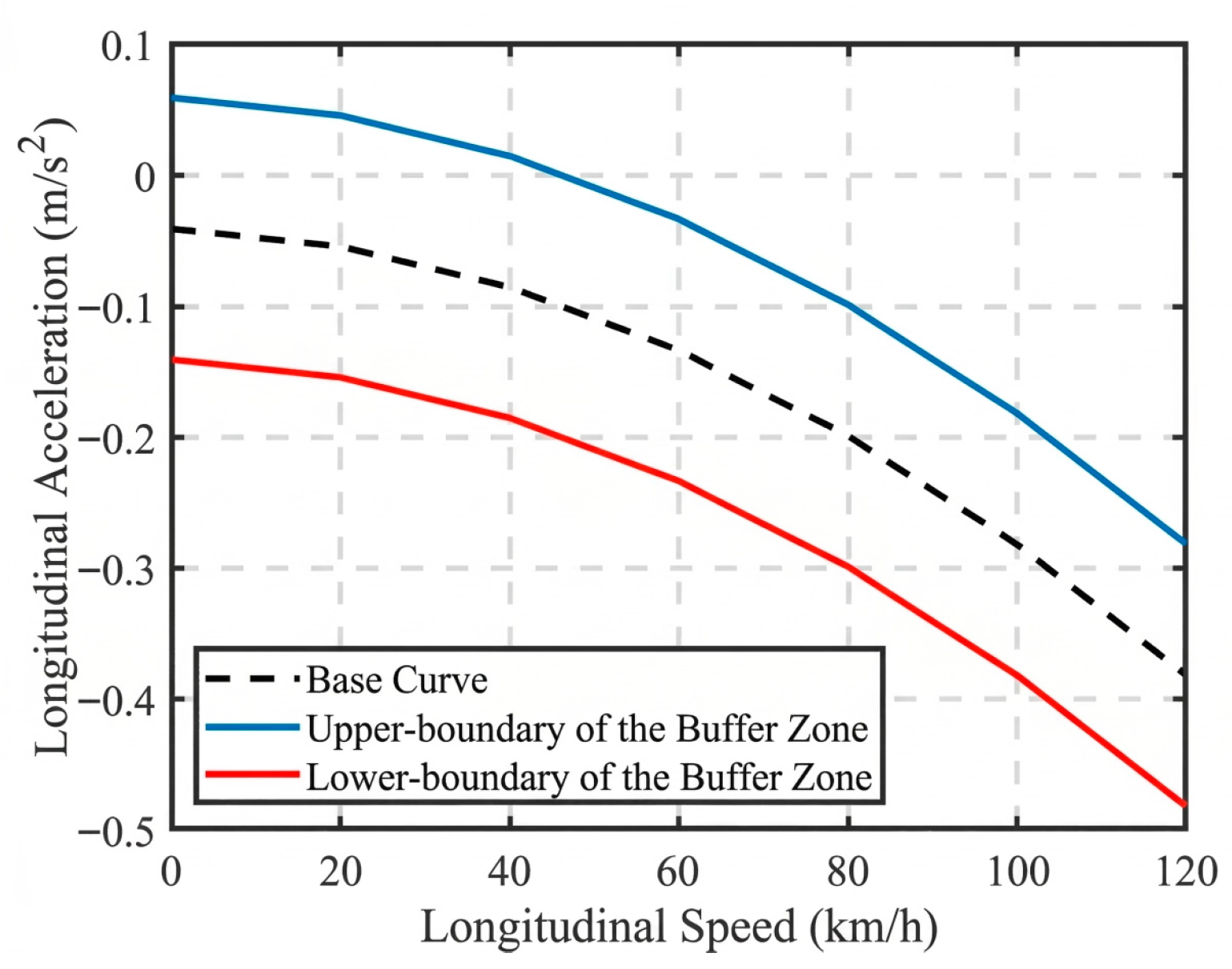
First, a coasting-down test is performed in CarSim R2022 under ideal road conditions at various vehicle speeds to determine the vehicle’s maximum deceleration during idle coasting. Then, the driving/braking switching base line at different vehicle speeds is obtained via curve fitting, as indicated by the dashed line in Figure 6. Next, to avoid frequent switching between driving and braking modes, buffer zones with a width of 0.1 m/s2 are set on either side of the base line, thus suppressing excessive acceleration and deceleration. The blue and red solid lines in Figure 6 denote the upper and lower boundaries of the buffer zones.
Briefly, at a specific vehicle speed, if the desired acceleration output from the upper controller exceeds the upper boundary in Figure 6, the system will switch to the driving mode. Otherwise, it will switch to the braking mode. If the desired acceleration falls in the buffer zone, the current mode will not be switched.

3.3.2. PI Controller

To align with the discrete-time implementation of the upper-level MPC controller, the longitudinal lower-level controller is designed as a discrete-time PI structure, as detailed below.
The longitudinal lower-level controller adopts a discrete-time PI control structure, implemented with a fixed sampling period T s = 0.01 to ensure consistency with the upper-level discrete MPC controller and the simulation environment.
The continuous-time PI control law is given by the following:
u a t = K P e a t + K I 0 t e a τ d τ
where e a t = a d e s t a a c t t denotes the acceleration tracking error, and K P and K I are proportionality gain and integral gain, respectively.
To realize this in digital implementation, the backward Euler method is used for discretization. The discrete-time PI control law is derived as follows:
u a k = u a k 1 + K P e a k e a k 1 + K I T s e a k
where k denotes the discrete time step, T s is the sampling period (consistent with the MPC prediction horizon), e a k = a d e s k a a c t k is the acceleration error at step k , and u a k is the control output at step k .
A joint simulation platform based on Matlab/Simulink R2022b and CarSim R2020 is used to conduct the simulation. The relevant parameters are shown in Table 2.

4. Simulation and Analysis

4.1. Simulation Analysis of Upper Controller

In this subsection, the MPC upper controller is simulated and proved. The linear quadratic regulator (LQR)-PID controller, which employs LQR for lateral path tracking and PID for longitudinal speed control, is adopted as the benchmark. For the simulation, the fifth-degree polynomial curve is used as the reference trajectory, the road adhesion coefficient is set to 0.85, the longitudinal spacing during lane change is 200 m, and the vehicle speed is 20 m/s. The results are given in Figure 7.
Figure 7a shows the reference trajectory and tracking performances of the two controllers. Figure 7b illustrates the lateral errors between the tracking paths of the two controllers and the reference path. In addition, the heading errors, front wheel steering angles, yaw rates, and sideslip angles of the two controlled vehicles are presented in Figure 7c–f.
As observed from Figure 7a, the two controllers can effectively enable the vehicle to track the reference trajectory. As shown in Figure 7b, the maximum lateral error of the MPC controller is approximately 0.008 m, whereas that of the LQR-PID controller is about 0.014 m. Similarly, Figure 7c illustrates that the maximum heading error of the MPC controller is around 0.0002 rad, while that of the LQR-PID controller is roughly 0.0004 rad. Compared with the LQR-PID controller, the MPC controller designed in this study reduced the maximum absolute values of lateral error and heading error by 42.9% and 50.0%. These results indicate that the MPC controller can constrain both lateral distance errors and heading errors within a smaller range.
It can be seen from Figure 7d that both controllers produce smooth front-wheel steering angles, free of sudden changes or significant fluctuations. Quantitatively, the MPC controller exhibits a maximum front-wheel steering angle of 0.00178 rad, which is slightly smaller than the LQR-PID controller’s 0.00193 rad. Compared with the LQR-PID controller, the MPC controller designed in this study reduced the maximum absolute value of the vehicle’s front-wheel steering angle by 7.8%. Figure 7e reveals that the yaw rates of the two controllers are highly consistent in trend and amplitude, with peaks coinciding with trajectory turning points; however, the MPC controller’s peak yaw rate is slightly lower than that of the LQR-PID controller. As presented in Figure 7f, the MPC controller generates a smaller peak sideslip angle (0.00026 rad) compared to the LQR-PID controller (0.00029 rad). Compared with the LQR-PID controller, the MPC controller designed in this study reduced the maximum absolute values of the vehicle’s yaw rate and sideslip angle by 2.8% and 10.3%. Collectively, these findings confirm that the MPC controller offers enhanced driving stability and operational smoothness for the vehicle.
To summarize, the lateral–longitudinal integrated MPC controller developed in this study exhibits superior control effectiveness compared to the LQR-PID controller when applied to trajectory tracking of a conventional-steered IWM-EV.

4.2. Simulation Analysis of Hierarchical Controller

Section 4.1 confirmed the upper controller’s satisfactory performance. Next, two IWM-EV setups are compared: a conventional steering EV with the MPC controller and the feedforward–feedback longitudinal controller (MPC + LC for short), and a differential steering EV with the MPC controller and the lateral and longitudinal lower controllers (MPC + LLC for short).
For the simulation, a two-lane straight road is adopted. Key parameters are configured as follows: the lateral displacement of the lane change trajectory is 3.75 m, the road adhesion coefficient is 0.85, and the longitudinal lane change distance is 90 m. Specifically, an accelerated lane change scenario is designed, where the vehicle’s longitudinal speed increases from an initial 15 m/s to a desired 20 m/s during the lane change process. The comparative simulation results are presented in Figure 8.
As can be seen from Figure 8a, both controllers can effectively enable the vehicle to track the reference trajectory under variable-speed conditions. Overall, the actual trajectory of the MPC + LLC controller is closer to the reference trajectory during the entire lane change process.
As observed from Figure 8b,c, the MPC + LLC controller limits the maximum lateral error to approximately 0.046 m and the maximum heading error to 0.0042 rad. In contrast, the MPC + LC controller exhibits slightly higher maximum values, with 0.056 m for lateral error and 0.0045 rad for heading error. Compared with the MPC + LC controller, the MPC + LLC controller designed in this study reduced the maximum absolute values of the lateral displacement error and heading error by 17.9% and 6.7%. These results indicate that the MPC + LLC controller achieves higher trajectory tracking accuracy than the MPC + LC controller.
As illustrated in Figure 8d, the yaw rate of the MPC + LLC controller is more consistent with the desired values compared to the MPC + LC controller. Compared with the MPC + LC controller, the MPC + LLC controller designed in this study reduced the maximum absolute value of the vehicle’s yaw rate by 33.3%. As shown in Figure 8e, the actual speed of the vehicle is highly consistent with the desired speed most of the time; the only deviation occurs during the lane change acceleration phase, with a maximum speed error of 0.27 m/s, which can be neglected. Additionally, the speed adjustment process is smooth without abrupt changes. These results demonstrate that the MPC + LLC controller fully meets the requirements for longitudinal control.
All in all, the proposed MPC + LLC controller achieves trajectory tracking with a maximum lateral error of 0.046 m and a maximum heading error of 0.0042 rad, compared to 0.056 m and 0.0045 rad for the MPC + LC controller. The yaw rate remains closer to the desired value, and the longitudinal speed error is limited to a maximum of 0.27 m/s during acceleration. These results indicate that the hierarchical controller provides improved tracking accuracy and maintains vehicle stability and ride comfort, even under differential steering under lane change conditions.

5. Conclusions

In this study, an MPC controller is proposed to jointly optimize the front-wheel steering angle and longitudinal acceleration for integrated longitudinal speed tracking and lateral path tracking. Moreover, an MFAC is adopted to achieve precise tracking of the desired front-wheel steering angle via differential steering, and a feedforward–feedback controller is developed to resolve the required rear-wheel drive torque or braking force from the longitudinal acceleration. The effectiveness of the constructed upper controller and the hierarchical control system is confirmed through co-simulation.
Compared with the LQR-PID controller, the MPC controller designed in this study reduced the maximum absolute values of lateral error and heading error by 42.9% and 50.0%, the vehicle’s front-wheel steering angle by 7.8%, and the vehicle’s yaw rate and sideslip angle by 2.8% and 10.3%. Compared with the MPC + LC controller, the MPC + LLC controller designed in this study reduced the maximum absolute values of the lateral displacement error and heading error by 17.9% and 6.7%, and the vehicle’s yaw rate by 33.3%.
Although the proposed method performs well in both theoretical and simulation analyses, there are still several limitations and directions worthy of further investigation. First, this paper only verifies the effectiveness of the differential steering control logic under ideal conditions. In future work, we will conduct research under more challenging working conditions (such as low road adhesion and more aggressive lane change maneuvers) to fully demonstrate the robustness of the proposed method. Second, the current design does not fully consider the potential influence of actuator saturation under large torque or steering demands, which may degrade control performance in extreme scenarios. Third, the proposed approach exhibits a certain degree of sensitivity to road friction variation, which could affect the differential steering performance under low-μ road conditions. Fourth, the current design relies on ideal assumptions regarding measurement noise and state estimation accuracy, and the robustness against noise and estimation errors needs further verification in practical applications. In addition, the verification in this paper is mainly carried out through simulations in a computer environment, and further real-vehicle experiments are needed in the future to validate the practical feasibility of the proposed method.

Author Contributions

Conceptualization, validation, and methodology, R.A.; methodology and writing—original draft preparation, H.M.; writing—original draft preparation, J.T.; writing—review and editing, R.A., J.T., H.M. and J.M.; funding acquisition, J.T. All authors have read and agreed to the published version of the manuscript.

Funding

This work was supported by the National Natural Science Foundation of China (51975299). This research was also funded by the Jiangsu Provincial Department of Science and Technology (BE2022053-2).

Institutional Review Board Statement

Not applicable.

Informed Consent Statement

Not applicable.

Data Availability Statement

The data used in this analysis are available on request from the corresponding author.

Acknowledgments

The authors wish to thank Tong Wu, Yupeng Su and Chenyu Huang for their valuable contribution and kind support to this study.

Conflicts of Interest

The authors declare no conflicts of interest.

Appendix A

Due to the nonlinearity, parameter time variation and uncertainty of the four-wheel distributed drive electric vehicle (FWDSV), a model-free adaptive control (MFAC) scheme is employed for the lateral lower-level control, as illustrated in the overall control framework (Figure 1). This approach aims to reduce the controller’s dependence on precise vehicle system models or complex mathematical representations, relying only on input and output data for online control adjustment. The detailed design process and theoretical derivation of the MFAC algorithm are presented as follows.
During the research, the FWDSV model (Equation (16)) can be regarded as a dual-input dual-output nonlinear discrete-time system:
Z k + 1 = f Z k , Z k 1 , , Z k n Z , U k , U k 1 , , U k n U ,
where U k p and Z k p denote the system’s input and output vectors, n U and n Z are unknown integers, and f = f 1 , , f 2 T n U + n Z + 2 p p is the unknown nonlinear function vector.
Given the continuous variation in the front left and right wheel driving torques and bounded input and bounded output (BIBO) stability constraints, two assumptions are made, as follows:
Assumption A1.
f i , i = 1 , , p  has continuous partial derivatives with respect to each component of the  n Z + 2 -th variable.
Assumption A2.
The system (as shown in Equation (A1)) satisfies the generalized Lipschitz condition; i.e., for any  k 1 k 2  with  k 1 , k 2 0  and  U k 1 U k 2 , the following relationship holds:
Z k 1 + 1 Z k 2 + 1 b ¯ U k 1 U k 2 ,
where  Z k i + 1 = f Z k i , , Z k i n Y , U k i , , U k i n U , and  b ¯  is a positive constant.
Theorem A1.
For the nonlinear discrete-time system (Equation (31)) satisfying Assumptions A1 and A2, a pseudo-Jacobian matrix (PJM)  Φ c k p × p  exists for any k with  Δ U k 0 , such that Equation (A2) can be transformed into a compact-form dynamic linearization model.
Δ Z k + 1 = Φ c k Δ U k ,   Φ c k ζ ,
where  Φ c k = ϕ 11 k ϕ 12 k ϕ 1 p k ϕ 21 k ϕ 22 k ϕ 2 p k ϕ p 1 k ϕ p 2 k ϕ p p k p × p .
We considered the following control input criterion function:
J U k = Z * k + 1 Z k + 1 2 + λ U k U k 1 2 ,
where λ > 0 is a weight factor, which balances tracking error and control effort. A larger λ imposes a heavier penalty on control input variations, yielding smoother control signals at the cost of a potentially slower transient response. In this work, λ = 0.5 is chosen to strike a favorable trade-off between tracking accuracy and control smoothness, and Z * k + 1 denotes the desired output signal.
Substitute Equation (A3) into Equation (A4), take the derivative of J U k with respect to U k and set it to zero; the simplified control algorithm is then obtained as follows:
U k = λ I + Φ c T k Φ c k 1 Φ c T k Z * k + 1 Z k + U k 1 .
Define the following parameter estimation criteria function:
J Φ c k = Δ Z k Φ c k Δ U k 1 2 + μ Φ c k Φ ^ c k 1 2 ,
where μ > 0 is a weighting factor, which governs the convergence speed of the pseudo-Jacobian matrix (PJM) estimation. A smaller μ accelerates adaptation but may introduce more estimation noise. We set μ = 10 4 to ensure stable and rapid convergence of the PJM estimation.
By minimizing the estimation criterion function in Equation (A6), the estimation algorithm for Φ c k is derived as follows:
Φ ^ c k = η 1 Δ Z k Φ ^ c k Δ U k 1 Δ U T k 1 μ + Δ U k 1 2 + Φ ^ c k 1 ,
where η 1 0 , 2 is the step size factor, which directly affects the convergence rate of the PJM. We choose η 1 = 1 to ensure the estimation error converges to zero within a reasonable number of time steps.
By estimating Φ c k , Equation (A5) can be rewritten as follows:
U k = U k 1 + ρ Φ ^ c T k Z * k + 1 Z k λ + Φ ^ c k 2 ,
where ρ 0 , 1 is the step size factor, which determines the aggressiveness of the control action. A larger ρ improves tracking speed but may induce oscillations. Here, ρ = 0.7 is selected to guarantee stable and reliable tracking performance.
To ensure the PJM variation remains within a reasonable range, a reset mechanism is introduced in this paper: when sgn Φ ^ c k sgn Φ ^ c 1 or Φ ^ c k ε |, reset Φ ^ c k to Φ ^ c 1 .
Define the system output error as follows:
e k = Z * k Z k .
By combining Equation (A1), it can be proved that under the joint action of Equations (A7) and (A8), the control error of the FWDSV satisfies the following condition:
lim k e = 0 .
Proof. 
Let Φ ^ c k = Φ ^ 1 T k , , Φ ^ p T k T , where Φ ^ i k = ϕ ^ i 1 k , ϕ ^ i p k for i = 1 , , p . Then, Equation (A7) can be rewritten as follows:
Φ ^ i k = η 1 Δ Z i k Φ ^ i k Δ U k 1 Δ U T k 1 μ + Δ U k 1 2 + Φ ^ i k 1 ,
where Δ Z i k = Φ i k 1 Δ U k 1 for i = 1 , , p .
Let Φ ˜ i k = Φ ^ i k Φ i k . Subtract Φ i k from both sides of Equation (A11); we then obtain the following:
Φ ˜ i k = Φ ˜ i k 1 + Φ i k 1 Φ i k η 1 Φ ˜ i k 1 Δ U k 1 Δ U T k 1 μ + Δ U k 1 2 .
By Theorem A1, Φ ^ c k is bounded, i.e., there exists a positive constant b ¯ such that Φ c k b ¯ . Thus, Φ i k 1 Φ i k 2 b ¯ . Taking the norm on both sides of Equation (A12) gives the following:
Φ ˜ i k = Φ ˜ i k 1 I η 1 Δ U k 1 Δ U T k 1 μ + Δ U k 1 2 + 2 b ¯ .
Squaring the first term on the right-hand side of Equation (A13) yields the following:
Φ ˜ i k 1 I η 1 Δ U k 1 Δ U T k 1 μ + Δ U k 1 2 2 = Φ ˜ i k 1 2 + 2 + η 1 Δ U k 1 2 μ + Δ U k 1 2 η 1 Φ ˜ i k 1 Δ U k 1 2 μ + Δ U k 1 2 0 .
For 0 < η 1 2 and μ > 0 , the following inequality holds:
2 + η 1 Δ U k 1 2 μ + Δ U k 1 2 0 .
From Equations (A14) and (A15), there exists 0 < d 1 < 1 such that the following is true:
Φ ˜ i k 1 I η 1 Δ U k 1 Δ U T k 1 μ + Δ U k 1 2 d 1 Φ ˜ i k 1 .
Substituting Equation (A16) into Equation (A13) gives the following:
Φ ˜ i k d 1 Φ ˜ i k 1 + 2 b ¯ d 1 2 Φ ˜ i k 2 + 2 d 1 b ¯ + 2 b ¯ d 1 k 1 Φ ˜ i 1 + 2 b ¯ 1 d 1 k 1 1 d 1 .
This implies that Φ ˜ i k is bounded. By Theorem A1, Φ i k is also bounded. Thus, Φ ^ i k and Φ ^ c k are bounded.
As k , the output Z * k of the ideal vehicle steering model exhibits steady-state behavior (i.e., Z * k + 1 = Z * k ). Combining Equations (A3) and (A8) gives the following:
e k + 1 = 1 ρ Φ c k Φ ^ c T k λ + Φ ^ c k 2 e k .
Since ρ 0 , 1 , and λ > 0 , we have the following equation:
1 ρ Φ c k Φ ^ c T k λ + Φ ^ c k 2 0 , 1 .
From Equations (A18) and (A19), we deduce that
lim k e k = 0 .

References

  1. Zhao, W.Z.; Zhang, H. Coupling Control Strategy of Force and Displacement for Electric Differential Power Steering System of Electric Vehicle with Motorized Wheels. IEEE Trans. Veh. Technol. 2018, 67, 8118–8128. [Google Scholar] [CrossRef]
  2. Sung, J.; Choi, S.; Huh, K. A Differential Brake-Actuated Steering System for Redundancy of Steer-by-Wire. IEEE Trans. Intell. Veh. 2024, 9, 993–1004. [Google Scholar] [CrossRef]
  3. Kuslits, M.; Bestle, D. Modelling and Control of a New Differential Steering Concept. Veh. Syst. Dyn. 2018, 57, 520–542. [Google Scholar] [CrossRef]
  4. Peng, D.Z.; Huang, B.; Huang, H. Design of an Anti-Windup PID Algorithm for Differential Torque Steering Systems. Shock. Vib. 2022, 1, 9973379. [Google Scholar] [CrossRef]
  5. Hu, C.; Wang, R.R.; Yan, F.J.; Huang, Y.; Wang, H.; Wei, C. Differential steering based yaw stabilization using ISMC for independently actuated electric vehicles. IEEE Trans. Intell. Transp. Syst. 2017, 19, 627–638. [Google Scholar] [CrossRef]
  6. Chen, T.; Cai, Y.F.; Chen, L.; Xu, X.; Sun, X. Trajectory tracking control of steer-by-wire autonomous ground vehicle considering the complete failure of vehicle steering motor. Simul. Model. Pract. Theory 2021, 109, 102235. [Google Scholar] [CrossRef]
  7. Omeiza, D.; Webb, H.; Jirotka, M.; Kunze, L. Explanations in Autonomous Driving: A Survey. IEEE Trans. Intell. Transp. Syst. 2022, 23, 10142–10162. [Google Scholar] [CrossRef]
  8. Guo, H.Y.; Shen, C.F.; Zhang, H.; Chen, H.; Jia, R. Simultaneous Trajectory Planning and Tracking Using an MPC Method for Cyber-Physical Systems: A Case Study of Obstacle Avoidance for an Intelligent Vehicle. IEEE Trans. Ind. Inform. 2018, 14, 4273–4283. [Google Scholar] [CrossRef]
  9. Wang, Z.P.; Sun, Z.Y.; Liu, P.; Wang, S.; Zhang, Z. Intelligent decision support platform of new energy vehicles. J. Syst. Eng. Electron. 2022, 33, 785–791. [Google Scholar] [CrossRef]
  10. Shen, K.; Ke, X.Y.; Yang, F.; Wang, W.; Zhang, C.; Yuan, C. Numerical Energy Analysis of In-Wheel Motor Driven Autonomous Electric Vehicles. IEEE Trans. Transp. Electrif. 2023, 9, 3662–3676. [Google Scholar] [CrossRef]
  11. Li, H.L.; Luo, Y.T. Integrated Coordination Control for Distributed Drive Electric Vehicle Trajectory Tracking. Int. J. Automot. Technol. 2020, 21, 1047–1060. [Google Scholar] [CrossRef]
  12. You, F.; Zhang, R.H.; Lie, G.; Wang, H.; Wen, H.; Xu, J. Trajectory planning and tracking control for autonomous lane change maneuver based on the cooperative vehicle infrastructure system. Expert Syst. Appl. 2015, 42, 5932–5946. [Google Scholar] [CrossRef]
  13. Zhang, C.Y.; Chu, D.F.; Liu, S.D.; Deng, Z.; Wu, C.; Su, X. Trajectory planning and tracking for autonomous vehicle based on state lattice and model predictive control. IEEE Intell. Transp. Syst. Mag. 2019, 11, 29–40. [Google Scholar] [CrossRef]
  14. Zhang, J.; Wu, J.; Shen, X.H.; Li, Y. Autonomous land vehicle path planning algorithm based on improved heuristic function of A-Star. Int. J. Adv. Robot. Syst. 2021, 18, 239094335. [Google Scholar] [CrossRef]
  15. Zeng, D.Q.; Yu, Z.P.; Xiong, L.; Zhao, J.Q.; Zhang, P.Z.; Li, Z.Q.; Fu, Z.Q.; Yao, J.; Zhou, Y. A Novel Trajectory Planning Method for Autonomous Vehicle Lane Change Based on B-Spline and RRT. In Proceedings of the IEEE Intelligent Vehicles Symposium (IV), Paris, France, 9–12 June 2019; pp. 486–493. [Google Scholar]
  16. Yao, Z.H.; Deng, H.W.; Wu, Y.X.; Zhao, B.; Li, G.; Jiang, Y. Optimal lane-changing trajectory planning for autonomous vehicles considering energy consumption. Expert Syst. Appl. 2023, 225, 120133. [Google Scholar] [CrossRef]
  17. Kou, Y.K.; Ma, C.X. Dual-objective intelligent vehicle lane changing trajectory planning based on polynomial optimization. Phys. A Stat. Mech. Its Appl. 2023, 617, 128665. [Google Scholar] [CrossRef]
  18. Yue, M.; Hou, X.Q.; Zhao, X.D.; Wu, X. Robust tube-based model predictive control for lane change maneuver of tractor-trailer vehicles based on a polynomial trajectory. IEEE Trans. Syst. Man Cybern. Syst. 2020, 50, 5180–5188. [Google Scholar] [CrossRef]
  19. Ding, Y.; Zhuang, W.C.; Wang, L.M.; Liu, J.; Guvenc, L.; Li, Z. Safe and optimal lane-change path planning for automated driving. J. Automob. Eng. 2021, 235, 1070–1083. [Google Scholar] [CrossRef]
  20. Chen, Y.X.; Peng, H.; Grizzle, J.W. Fast Trajectory Planning and Robust Trajectory Tracking for Pedestrian Avoidance. IEEE Access 2017, 5, 9304–9317. [Google Scholar] [CrossRef]
  21. Luo, Z.; Zheng, Y. Analyzing the impact of wind on trajectory tracking for unmanned vehicles based on road adhesion coefficient estimation. Processes 2025, 13, 52. [Google Scholar] [CrossRef]
  22. Yao, J.; Ge, Z. Path-tracking control strategy of unmanned vehicle based on DDPG algorithm. Sensors 2022, 22, 7881. [Google Scholar] [CrossRef]
  23. Li, P.; Wei, L.; Wu, D. An intelligently enhanced ant colony optimization algorithm for global path planning of mobile robots in engineering applications. Sensors 2025, 25, 1326. [Google Scholar] [CrossRef]
  24. Zhang, Y.; Liu, K.; Gao, F.; Zhao, F. Research on path planning and path tracking control of autonomous vehicles based on improved APF and SMC. Sensors 2023, 23, 7918. [Google Scholar] [CrossRef]
  25. Zhang, Y.; Gao, F.; Zhao, F. Research on path planning and tracking control of autonomous vehicles based on improved RRT* and PSO-LQR. Processes 2023, 11, 1841. [Google Scholar] [CrossRef]
  26. Carlucho, I.; De Paula, M.; Acosta, G.G. An adaptive deep reinforcement learning approach for MIMO PID control of mobile robots. ISA Trans. 2020, 102, 280–294. [Google Scholar] [CrossRef] [PubMed]
  27. Kapania, N.R.; Gerdes, J.C. Design of a feedback-feedforward steering controller for accurate path tracking and stability at the limits of handling. Veh. Syst. Dyn. 2015, 53, 1687–1704. [Google Scholar] [CrossRef]
  28. Huang, K.; Jiang, C.; Qiu, M.; Wu, D.; Zhang, B.Z. Research on intelligent vehicle lane changing and obstacle avoidance control based on road adhesion coefficient. J. Vib. Control. 2022, 28, 3269–3285. [Google Scholar] [CrossRef]
  29. Li, Z.H.; Wang, P.; Liu, H.H.; Hu, Y.; Chen, H. Coordinated longitudinal and lateral vehicle stability control based on the combined-slip tire model in the MPC framework. Mech. Syst. Signal Process. 2021, 161, 107947. [Google Scholar] [CrossRef]
  30. Sun, Z.Y.; Wang, R.C.; Ye, Q.; Wei, Z.; Yan, B. Investigation of Intelligent Vehicle Path Tracking Based on Longitudinal and Lateral Coordinated Control. IEEE Access 2020, 8, 105031–105046. [Google Scholar] [CrossRef]
  31. Park, H.; Gerdes, J.C. Optimal tire force allocation for trajectory tracking with an over-actuated vehicle. In Proceedings of the IEEE Intelligent Vehicles Symposium, Seoul, Republic of Korea, 28 June–1 July 2015; pp. 1032–1037. [Google Scholar]
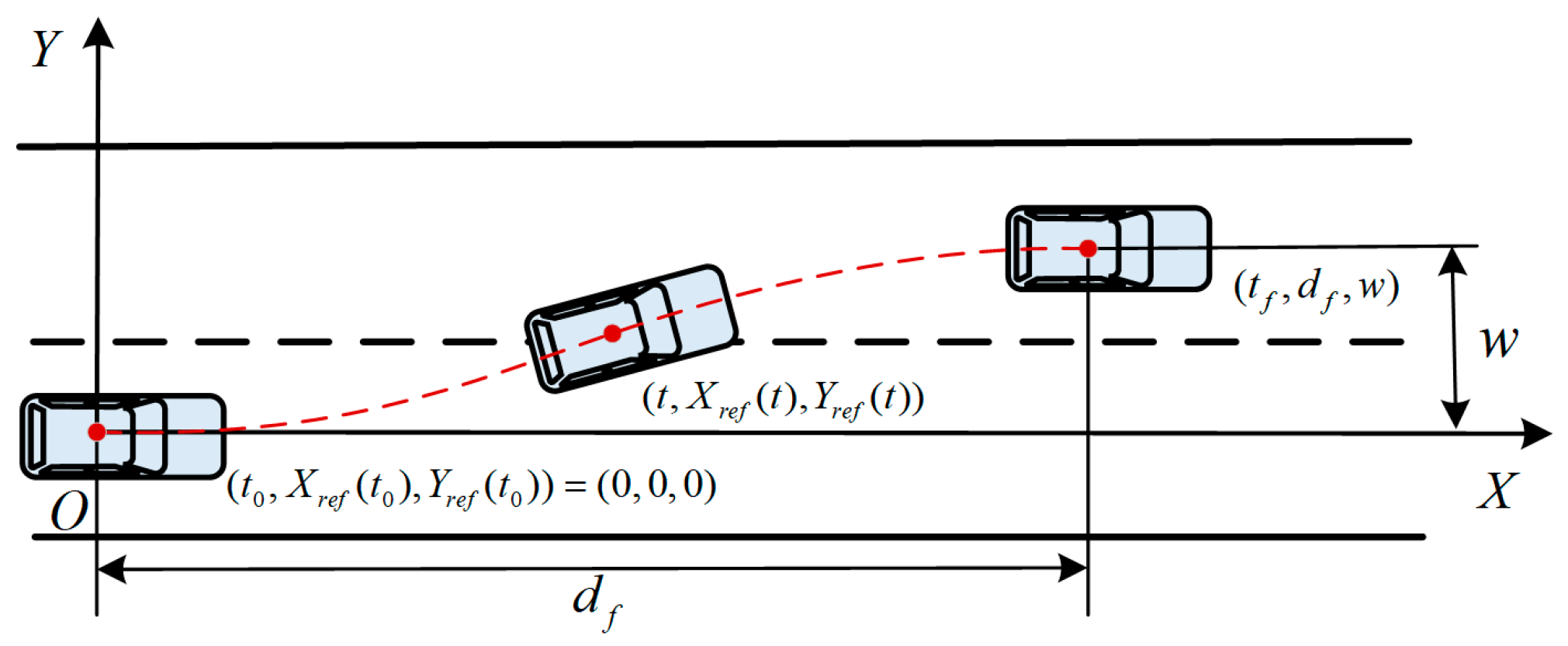
Figure 2. Schematic of lane change trajectory. In this figure: the red dashed line represents the planned lane-change trajectory of the vehicle; the black dashed line denotes the lane centerline; the solid black lines indicate the road edges, and the red dots mark the vehicle’s CG position.
Actuators 15 00205 g002
Figure 3. Lateral trajectory tracking. In this figure: the black solid curve represents the reference trajectory, with the yellow point marking the reference position; the red arrows denote the vehicle’s velocity, tire forces, and other dynamic vectors; the blue solid lines with double arrows indicate the position deviation ( Δ X , Δ Y ); and the black dashed lines represent the reference baselines.
Actuators 15 00205 g003
Figure 4. FWDSV dynamics model.
Actuators 15 00205 g004
Figure 5. Schematic of FWDSS. In this figure, the red arrows denote the torque acting on the steering system; and the black arrows denote the force vectors acting on the front tires.
Actuators 15 00205 g005
Figure 6. Drive/brake switching curve.
Actuators 15 00205 g006
Figure 7. Simulation results of upper controllers. (a) Trajectory tracking curve; (b) lateral error; (c) heading error; (d) front-wheel steering angle; (e) yaw rate; (f) sideslip angle.
Actuators 15 00205 g007
Figure 8. Comparative simulation results of hierarchical controllers. (a) Trajectory tracking results; (b) lateral error; (c) heading error; (d) yaw rate; (e) sideslip angle.
Actuators 15 00205 g008
Table 2. Related parameters.
SymbleValueSymbleValue
m 1413 kg N p 10
a 1.015 m N c 5
b 1.895 m T s 0.1 s
I z 1536.7 kgm2 δ f min −0.523 rad
C f −148,970 N/rad δ f max 0.523 rad
C r −82,204 N/rad a max 5 m/s2
R 0.347 m a min −5 m/s2
Disclaimer/Publisher’s Note: The statements, opinions and data contained in all publications are solely those of the individual author(s) and contributor(s) and not of MDPI and/or the editor(s). MDPI and/or the editor(s) disclaim responsibility for any injury to people or property resulting from any ideas, methods, instructions or products referred to in the content.