Modeling and Adaptive Control of Biped Robots

Abstract

This study presents the design and performance evaluation of an adaptive control system for a biped robot with five degrees of freedom. The primary goal is to achieve stable and accurate control despite uncertainties in the robot’s dynamic parameters and changes in environmental conditions. By analyzing the robot’s dynamic structure, an adaptive control strategy is developed, and its effectiveness is assessed through simulations. The results indicate that the proposed approach delivers superior performance. In particular, the system’s ability to update dynamic parameters in real time significantly reduces tracking errors and ensures the robot’s stability under uncertain conditions. Based on a passivity-based control framework commonly referenced in the literature, the adaptive controller enables precise tracking of desired reference signals, even in complex dynamic environments. Overall, the findings demonstrate that adaptive control is a highly effective solution, especially for complex systems such as biped robots.

1. Introduction

In this study, an efficient and optimized dynamic control strategy for bipedal robots using adaptive methods is presented. Based on the evaluations conducted in the literature review, it is evident that the proposed control approach is inspired by biological structures observed in human locomotion, distinguishing it from many existing gait control methods applied to legged robots.

The walking patterns of humanoid bipedal robots have been extensively investigated by researchers [1,2], with the primary goal of replicating human-like motion as closely as possible. Human locomotion is inherently energy-efficient and balanced. In recent years, studies focusing on the mobility and degrees of freedom (DoF) of bipedal robots have gained considerable attention [1,2,3]. One widely used approach to generate human-like motion is through optimization techniques. For instance, in [4], an energy optimization strategy based on the zero moment point (ZMP) criterion was proposed to address the challenge of high energy consumption, particularly in unstructured environments.

Another common approach for generating motion signals is to derive reference trajectories from detailed analyses of human walking patterns [5,6,7]. Furthermore, motion trajectories of the ankle and hip joints can be determined using workspace analysis, inverse kinematics, and dynamic stability criteria.

A key characteristic of human locomotion is the ability to adapt to environmental changes by modifying gait parameters such as walking speed and step length in real time. In [8], a method based on a genetic algorithm and Fourier series was introduced to generate stable motion signals. Similarly, ref. [9] proposed a motion path design approach for bipedal robots with variable step lengths, while [10] presented a technique that adapts step length and gait cycle based on the linear inverted pendulum model.

Another strategy for designing motion paths is to use human motion data. However, recording joint angle trajectories over a wide range of step lengths and walking speeds can be technically challenging [11]. In [12], an AI-based motion planning method for a five-degree-of-freedom bipedal robot was introduced, utilizing a three-layer artificial neural network to generate control signals for each walking phase. Additionally, ref. [13] proposed a fuzzy logic-based method where a trained fuzzy neural network was used to produce motion signals based on a learned gait model. Goswami et al. applied the ZMP principle to control bipedal motion by incorporating motion signal generation and step rate control under stability constraints.

In recent years, the research community has shown increasing interest in developing bipedal robots capable of replicating human-like motion. This interest stems from the potential of bipedal robots to traverse uneven or irregular terrain—environments typically inaccessible to wheeled robots [14]. Applications for bipedal robots continue to expand, particularly in high-risk environments such as search and rescue missions [15], military operations and disaster response scenarios [16], and in the fields of prosthetics and rehabilitation robotics [17,18].

Despite growing interest, the advancement of bipedal robotics has been relatively slow due to the inherent complexity of its dynamic systems. This complexity increases significantly with the number of mechanical links and degrees of freedom [19]. Typically, the dynamic modeling of bipedal robots is performed using the Lagrangian energy approach. However, it is important to note that the computational complexity of the Lagrangian formulation scales as O(n_v³), where n_v denotes the number of degrees of freedom. Consequently, formulating dynamic models for three-dimensional systems with more than twelve degrees of freedom results in significantly lengthy and complex equations [20].

In recent years, there have been various distinctive and original studies conducted, particularly in the field of control systems. These include: Ref. [21] proposed a parameter-adaptive sliding mode control strategy based on a radial basis function neural network (RBFNN) for the trajectory tracking of a tilt-quadrotor unmanned aerial vehicle (TQUAV) with time-varying mass and uncertainties. The external disturbances and uncertainties were considered collectively as a total disturbance term, which was estimated using the RBFNN. Additionally, an adaptive control approach was employed to minimize tracking errors. The stability of the system was analyzed using a Lyapunov function, and the effectiveness of the proposed method was validated through computer simulations. Ref. [22] investigated the position tracking control of an upper-limb exoskeleton robot system mounted on a wheelchair, intended for the rehabilitation of individuals with disabilities. To achieve this, a fuzzy non-singular terminal sliding mode control method incorporating a fixed-time convergence rate state observer was designed in three main stages. First, a fixed-time state observer was proposed for state estimation. Second, the fixed-time convergence of the position tracking error of the upper-limb exoskeleton robot system was examined using a non-singular terminal sliding mode control approach. Third, to mitigate the adverse effects of vibration phenomena that degrade controller performance, a fuzzy control strategy was employed to enhance the system’s control effectiveness. The proposed control algorithm was implemented on an upper-limb multimodal human-exoskeleton robot system within the Matlab/Simulink environment. Ref. [23] proposed a trajectory tracking control strategy for robotic manipulators based on the fully actuated system (FAS) approach, which is commonly used in the design of nonlinear controllers. To address the system’s complexities, the dynamic model of the robotic manipulators was constructed using model identification techniques. Based on the identified model, a simplified FAS composite control strategy was designed by integrating a high-order disturbance observer (HODO) into the inner loop and an FAS-based trajectory tracking controller in the outer loop. To validate the performance of the proposed controller, both numerical simulations and experimental studies were conducted. In [24], the study investigated a prescribed performance adaptive robust control (PPARC) scheme for uncertain robotic manipulators. First, the system was transformed into a state-space representation. Second, the PPARC was developed to minimize tracking errors. Subsequently, a Lyapunov function was constructed for stability analysis. Furthermore, a fuzzy logic-based controller was designed. The proposed control strategy was tested in a computer simulation environment. Ref. [24] designed an adaptive non-singular terminal sliding mode control (NTSMC) technique based on a barrier function to enhance the performance and ensure robust stability of nonlinear systems under external disturbances. The stability of the system was guaranteed using a Lyapunov function. An adaptive technique was employed to estimate the unknown upper bounds of the external disturbances. Moreover, an adaptive neural network-based approach was implemented for fixed-time position tracking control of an upper-limb exoskeleton robot system mounted on a wheelchair, to protect it against external disturbances. In [25], the position tracking capability between the actual and desired trajectories of the exoskeleton system was then tuned. A terminal sliding mode controller was designed to reduce tracking errors. Additionally, an adaptive neural network model was developed to estimate the existing external disturbances affecting the operation of the upper-limb exoskeleton system. The effectiveness of the proposed method was validated through computer simulations. Ref. [26] introduced a multi-modal human–exoskeleton cooperative control strategy to enable smooth and stable switching between different control modes. Meanwhile, an adaptive backstepping controller with radial basis functions was designed to reduce tracking errors in the presence of model uncertainties. Finally, an experimental setup was developed to evaluate the performance of the proposed control strategy.

The key distinguishing feature of this study is the first-time application of the proposed control approach to a 5-DOF bipedal robot. The controller demonstrates robust performance even under external disturbances and uncertainties, which enhances its potential for real-world implementation in such robotic systems.

The Introduction section provides a comprehensive review of previous studies relevant to the topic. Section 2 presents the static and dynamic equations governing the motion of bipedal robots. Following this, an adaptive control strategy is introduced, and the control system is specifically formulated for application to bipedal robotic structures. The Results section includes computer simulations demonstrating the performance of the adaptive controller when applied to the bipedal robot model. Finally, the Discussion and Conclusion sections summarize the study, interpret the findings, and propose directions for future research.

2. Materials and Methods

In the study of bipedal robot locomotion, significant research has been conducted on their potential applications, particularly in challenging environments such as uneven terrain and stair navigation. Bipedal robots are utilized in a wide range of fields, including mine detection, nuclear power plant operations, and military interventions, often deemed hazardous for humans. Additionally, they play an important role in robotic rehabilitation for individuals with disabilities. Research on the walking principles of bipedal robots is expected to contribute to the development of dynamic models that can be applied to a broad range of bipedal robotic systems.

2.1. Model

2.1.1. Static Model

This static model describes the motion of a bipedal robot based on position, velocity, and acceleration angles. External forces, such as surface contact forces, that cause motion are not considered.

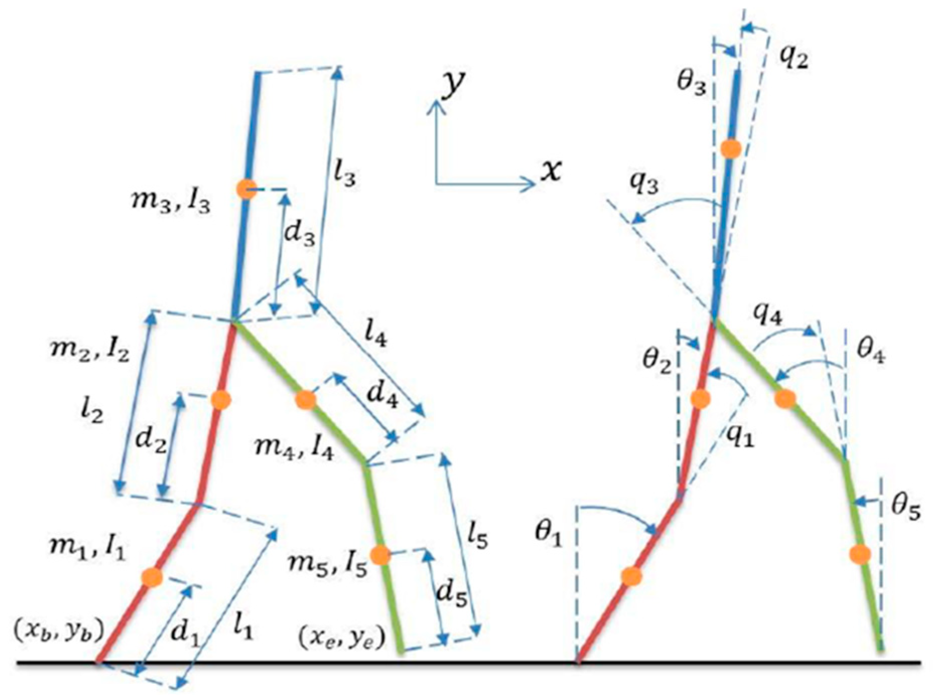
The bipedal robot studied has 5 joints and is limited to the sagittal plane. It consists of a half-body and two equal legs, each with 2 joints. All joints have rotational movement. The friction between the legs and the surface conditions is considered sufficient to prevent the risk of slipping. This robot has 4 actuators, 1 for each knee.

The parameters shown in Figure 1 are listed in abbreviations. The following formulas can be obtained from Figure 1.

$$x_e=x_b+l_1\mathit{sin}{\theta }_1+l_2\mathit{sin}{\theta }_2+l_4\mathit{sin}{\theta }_{4 }+l_5\mathit{sin}{\theta }_5$$

(1)

$$y_e=x_b+l_1\mathit{cos}{\theta }_1+l_2\mathit{cos}{\theta }_2-l_4\mathit{cos}{\theta }_{4 }-l_5\mathit{cos}{\theta }_5$$

(2)

If cgx and cgy are the center of mass coordinates of the biped robot, the center of mass coordinates of each link are:

$$x_{c1}=d_1\mathit{sin}{\theta }_1$$

(3)

$$y_{c1}=d_1\cos {\theta }_1$$

(4)

$$x_{c2}=l_1\mathit{sin}{\theta }_1+d_2\mathit{sin}{\theta }_2$$

(5)

$$y_{c2}=l_1\mathit{cos}{\theta }_1+d_2\mathit{cos}{\theta }_2$$

(6)

$$x_{c3}=l_1\mathit{sin}{\theta }_1+l_2\mathit{sin}{\theta }_2+d_3\mathit{sin}{\theta }_{3 }$$

(7)

$$y_{c3}=l_1\mathit{cos}{\theta }_1+l_2\mathit{cos}{\theta }_2+d_3\mathit{cos}{\theta }_{3 }$$

(8)

$$x_{c4}=l_1\mathit{sin}{\theta }_1+l_2\mathit{sin}{\theta }_2+(l_4-d_4)\mathit{sin}{\theta }_{4 }$$

(9)

$$y_{c4}=l_1\cos {\theta }_1+l_2\cos {\theta }_2-(l_4-d_4)\cos {\theta }_{4 }$$

(10)

$$x_{c5}=l_1\sin {\theta }_1+l_2\sin {\theta }_2+l_4\sin {\theta }_4+(l_5-d_5)\sin {\theta }_{5 }$$

(11)

$$y_{c5}=l_1\cos {\theta }_1+l_2\cos {\theta }_2-l_4\cos {\theta }_4-(l_5-d_5)\cos {\theta }_{5 }$$

(12)

$$cgx={\displaystyle \frac{m_{1 }{x}_{c1}+m_2{x}_{c2}+m_3{x}_{c3}+m_4{x}_{c4}+m_5{x}_{c5}}{m_{1 }+m_2+m_3+m_4+m_5}}$$

(13)

$$cgy={\displaystyle \frac{m_{1 }{y}_{c1}+m_2{y}_{c2}+m_3{y}_{c3}+m_4{y}_{c4}+m_5{y}_{c5}}{m_{1 }+m_2+m_3+m_4+m_5}}$$

(14)

2.1.2. Dynamic Model

In this work, the aim was to utilize a robot model that resembles human nature. For this reason, a 5-degree-of-freedom robot capable of dynamic behavior was employed. The dynamic model is used to calculate the torques applied to each joint, so all external forces are included in the dynamic model. The friction force is assumed to be sufficiently large to ensure that there is no slipping on the supporting base. The dynamic model is presented for single and two-phase cases. Since the motion of the biped robot occurs in the sagittal plane, the angles θi (i = 1, 2, …, 5) are sufficient to describe its posture completely. According to Lagrangian, the dynamic model for the SSP is:

$$\mathrm{D}\left(\theta \right)\ddot{\mathsf{\theta }}+\mathrm{H}\left(\mathsf{\theta }\right){\dot{\mathsf{\theta }}}^2+ \mathrm{G} \left(\mathsf{\theta }\right) = {\mathrm{T}}_{\mathsf{\theta }}$$

(15)

The matrix D(θ) represents an inertia matrix that shows the motion of the robot from a positive 5*5 specific and symmetric moment-to-moment transition. H(θ) is a 5*5 matrix that groups the centrifugal force and Coriolis terms; the centrifugal force is the radial forces and the Coriolis force shows the deviations from the rotational motion due to the rotational component. The matrix G(θ) represents a 5*5 gravity expression.

$$D_{ij}=p_{ij} cos({\theta }_i-{\theta }_j)$$

(16)

$$H_{ij}=p_{ij} \mathit{sin}\left({\theta }_i-{\theta }_j\right)$$

(17)

$$G_i=g_i sin\left({\theta }_i\right)$$

(18)

$$p_{ij}=\left\{\begin{array}{cc}{l}_i+m_i {d_i}^2+a_{i }\left({\sum }_{j=i+1}^5{m}_j\right), & i=j\\ a_{i }{m}_j{d}_j{l}_i+a_{i }{a}_{j }\left({\sum }_{k=j+1}^5{m}_k\right)l_i{l}_{j }, & j>i\\ p_{ij}, & j<i\end{array}\right.$$

(19)

$$g_i=m_i d_{i}g+a_{i }\left({\sum }_{j=i+1}^5{m}_j\right)l_{i}g$$

(20)

Here α(i) is a number defined as follows: if i = 3 then α(i) = 0, and if i = (1, 2, 4, 5) then α(i) = 1.

2.1.3. Double Support Stage and Switching

In the double support stage, the position between the end points of the links and the surface is fixed. Therefore, the algebraic equations representing the position constraints are as follows:

$$\varphi (\theta )=\left[\begin{array}{c}{f}_1\\ f_2\end{array}\right]=\left[\begin{array}{c}{x}_e-x_b-L \\ y_e-y_b\end{array}\right]=0$$

(21)

Here, L is the step length. Now, if we apply Lagrangian with constraints, the dynamic equation for DSP (double support phase) can be expressed as:

$$D\left(\mathsf{\theta }\right)\ddot{\theta } + H\left(\mathsf{\theta }\right){\dot{\mathsf{\theta }}}^2+ \mathrm{G} (\mathsf{\theta }) = J^T\left(\theta \right)\lambda + T_{\theta }$$

(22)

$$J=\left(\begin{array}{c}{l}_1{\cos \theta }_1\\ -l_1{\sin \theta }_1\end{array} \begin{array}{c}{l}_3{\cos \theta }_3\\ -l_1{\sin \theta }_1\end{array} \begin{array}{c}0\\ 0\end{array} \begin{array}{c}{l}_4{\cos \theta }_4\\ -l_4{\sin \theta }_4\end{array} \begin{array}{c}{l}_5{\cos \theta }_5\\ -l_5{\sin \theta }_5\end{array} \right)$$

(23)

As a result, we can rewrite the equation as follows;

$$\ddot{\theta }=D^{-1}\left( T_{\theta }-H\left(\mathsf{\theta }\right){\dot{\mathsf{\theta }}}^2-\mathrm{G}\left(\mathsf{\theta }\right)+J^T\lambda \right)$$

(24)

To ensure that the dynamic model works in the next cycle, the roles of the supporting leg and the rotating leg must be changed. The physical displacements and velocities do not actually change, but the name of the joint used in the dynamic model must be changed. The state immediately before and after the key change can be written as follows:

$$\left[\begin{array}{c}{\theta }^{+}\\ {\dot{\theta }}^{+}\end{array}\right] =\left[\begin{array}{cc}T& 0_{5\times 5}\\ 0_{5\times 5}& T\end{array}\right]\left[\begin{array}{c}{\theta }^{-}\\ {\dot{\theta }}^{+}\end{array}\right]$$

(25)

$$T=\left[\begin{array}{ccccc}0& 0& 0& 0& -1\\ 0& 0& 0& -1& 0\\ 0& 0& 0& 0& 0\\ 0& -1& 0& 0& 0\\ -1& 0& 0& 0& 0\end{array}\right]$$

(26)

To apply torque to the motor of each joint, the bipedal dynamics described throughout the DSP and SSP must be reformulated in terms of relative angles.

$$\begin{array}{c}{D}_q\left(q\right)\ddot{q}+H_q\left(q\right){\dot{q}}^2+G_q\left(q\right)=T_q\\ D_q\left(q\right)\ddot{q}+H_q\left(q\right){\dot{q}}^2+G_q\left(q\right)=J_q^T\left(q\right)\lambda +T_q\end{array}$$

(27)

2.1.4. Path Planning

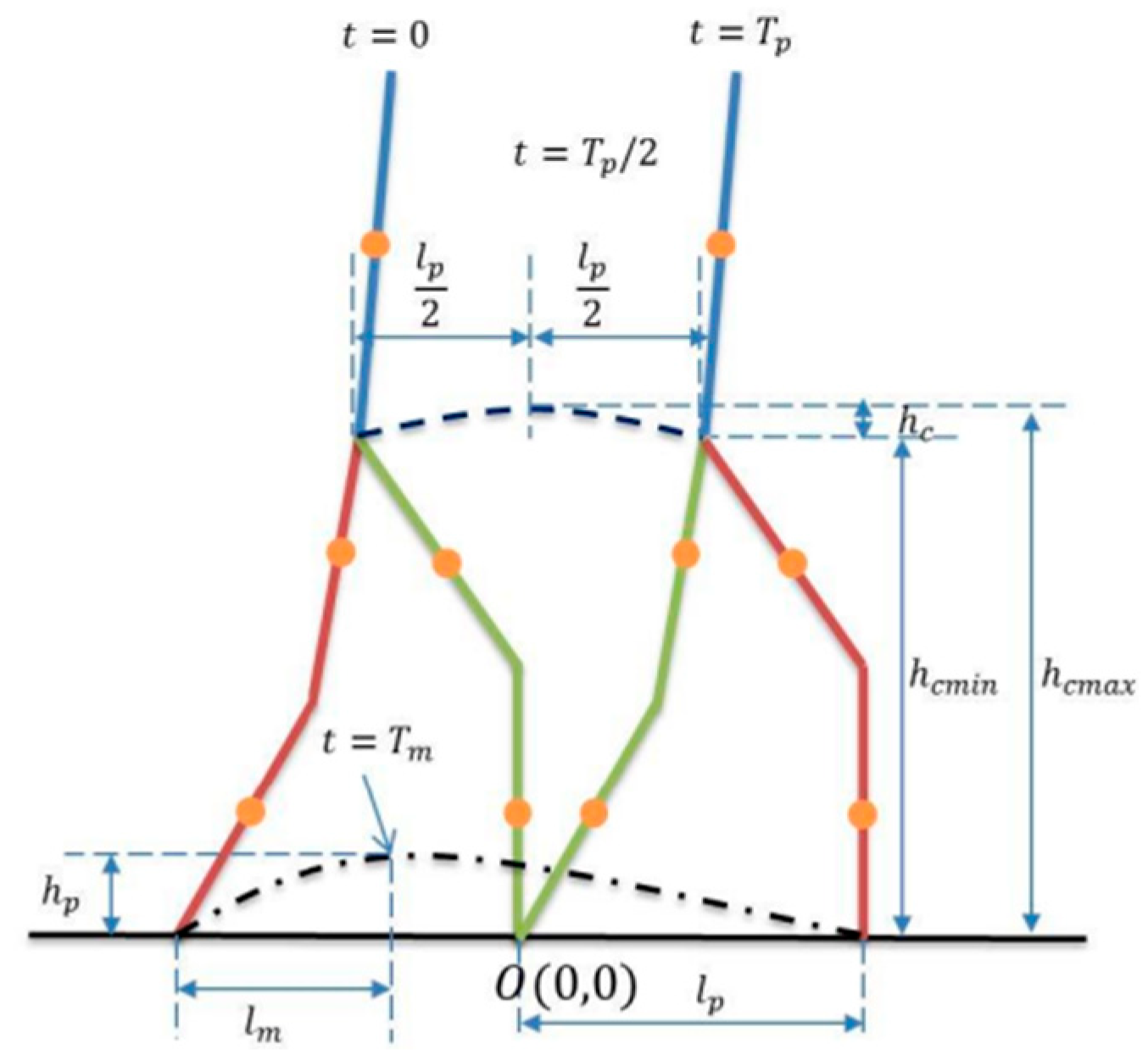
This section describes the method used to generate the path in the sagittal plane of the five-link biped robot. First, we obtain the path of the thigh and lower leg in the swing so that we can obtain the angles of each joint. The following Figure 2 shows the parameters required for gait planning in the sagittal plane. Here, T_p is the duration of one step, l_p is the step length, h_cmax is the maximum hip height, hl_m is the distance measured from the foot lift off the surface to the maximum height, and T_m is the time when the foot reaches the maximum height.

The robot’s foot motion path is denoted by (x_e(t), y_e(t)); the robot’s foot starts from (−lp, O) and reaches (−l_p + l_max, h_p) at time T_m. Then, it hits (l_p, O) at time T_p. On the other hand, the hip motion path is denoted by (x_c(t), y_c(t)); the hip starts from (lp/2, h_cmin), reaches (h_cmax, 0) at time T_p/2, and finally reaches (l_p/2, h_cmin) at time T_p. In order to minimize the surface impact effects that cause changes in the instantaneous angular velocity of the joints, the velocity at the moment of contact is reduced to zero. In addition, to ensure the repeatability of the walking path, the velocity at the beginning of the path should also be zero.

$$x_e\left(t\right)={\displaystyle \frac{-4l_p}{{T_p}^3}}{t}^3+{\displaystyle \frac{6l_p}{{T_p}^2}}{t}^2-l_p\hspace{1em}0<t\le T_p$$

(28)

$$y_e(t)=\left\{\begin{array}{cc}{\displaystyle \frac{-16h_p}{{T_p}^3}}{t}^3+{\displaystyle \frac{12h_p}{{T_p}^2}}{t}^2& 0<t\le T_p/2\\ {\displaystyle \frac{16h_p}{{T_p}^3}}{t}^3-{\displaystyle \frac{36h_p}{{T_p}^2}}{t}^2+{\displaystyle \frac{24h_p}{T_p}}t-4h_p& T_p/2<t\le T_p\end{array}\right.$$

(29)

$$x_c\left(t\right)={\displaystyle \frac{-2l_p}{{T_p}^3}}{t}^3+{\displaystyle \frac{3l_p}{{T_p}^2}}{t}^2-{\displaystyle \frac{l_p}{2}}\hspace{1em}0<t\le T_p$$

(30)

$$y_c(t)=\left\{\begin{array}{cc}{\displaystyle \frac{-16h_c}{{T_p}^3}}{t}^3+{\displaystyle \frac{12h_c}{{T_p}^2}}{t}^2+h_{cmin}& 0<t\le T_p/2\\ {\displaystyle \frac{16h_c}{{T_p}^3}}{t}^3-{\displaystyle \frac{36h_c}{{T_p}^2}}{t}^2+{\displaystyle \frac{24h_c}{T_p}}t+h_{cmin}-4h_c& T_p/2<t\le T_p\end{array}\right.$$

(31)

To obtain the paths shown in the figure above, the values in the

Table 1. Parameters of the paths obtained from human walking data.

Tp	Tm	Lp	hp	lmax	hcmin	hcmax
0.97 m	0.96 m	0.2 m	0.07 m	0.4 m	0.38 m	0.76 m

of data obtained from human walking were used.

The angle θ₃ is considered fixed and its value depends on the designer’s choice (usually it is assumed to be zero).

$$\begin{array}{ll} & {\theta }_1(t)=2{\mathrm{t}\mathrm{a}\mathrm{n}}^{-1}{\displaystyle \frac{2l_1{x}_c(t)+\sqrt{-{\left(l_1^2-l_2^2\right)}^2+2A\left(l_1^2+l_2^2\right)-A^2}}{l_1^2-l_2^2+2l_1{y}_c(t)+A}}\\ & {\theta }_2(t)=2{\mathrm{t}\mathrm{a}\mathrm{n}}^{-1}{\displaystyle \frac{2l_2{x}_c(t)-\sqrt{\left(-{\left(l_1^2-l_2^2\right)}^2+A\right)\left({\left(l_1^2+l_2^2\right)}^2-A\right)}}{-l_1^2+l_2^2+2l_2{y}_c(t)+A}}\\ & {\theta }_3(t)=0.04\\ & {\theta }_4(t)=2{\mathrm{t}\mathrm{a}\mathrm{n}}^{-1}{\displaystyle \frac{2l_{2}B+\sqrt{\left(-{\left(l_5^2-l_2^2\right)}^2+D\right)\left({\left(l_5^2+l_4^2\right)}^2-D\right)}}{-l_5^2+l_4^2+2l_{2}C+D}}\\ & {\theta }_5(t)=2{\mathrm{t}\mathrm{a}\mathrm{n}}^{-1}{\displaystyle \frac{2l_{1}B-\sqrt{-{\left(l_5^2-l_4^2\right)}^2+2D\left(l_5^2+l_4^2\right)-D^2}}{l_5^2-l_4^2+2l_{5}C+D}}\end{array}$$

(32)

2.2. Adaptive Controller Design for a Five-Degree-of-Freedom Biped Robot

In this section, the proposed system model for adaptive control of a biped robot with 5 degrees of freedom is described in detail. This model is based on both theoretical foundations and practical simulations to address the nonlinear and uncertain dynamics of the robot. Two main references were used in the design: the one presented by [28] and the one implemented using MATLAB [29]. Figure 3 presents the block diagram resulting from the implementation of the adaptive controller on the bipedal robot. The difference between the desired trajectory and the current state serves as the input to the controller. The resulting control force determines the robot’s position, which is then fed back into the system to form a closed-loop control structure.

Bipedal robots have quite complex dynamics during balancing and walking. Traditional control methods may be inadequate to cope with uncertainties in system parameters such as the robot’s mass, joint friction, and inertia. In this context, the adaptive control strategy aims to secure the stability and path-following performance of the robot by dynamically adapting to the uncertainties in the system.

The adaptive controller is based on Lyapunov stability theory and ensures the stability of the system as well as the convergence of the tracking error towards zero over time. In this study, the design and simulation of the adaptive controller are performed using MATLAB and Simulink environments, and the obtained results are compared. The main challenges encountered while controlling a bipedal robot are the correct modeling of the robot and the effective application of the torques generated by the controller.

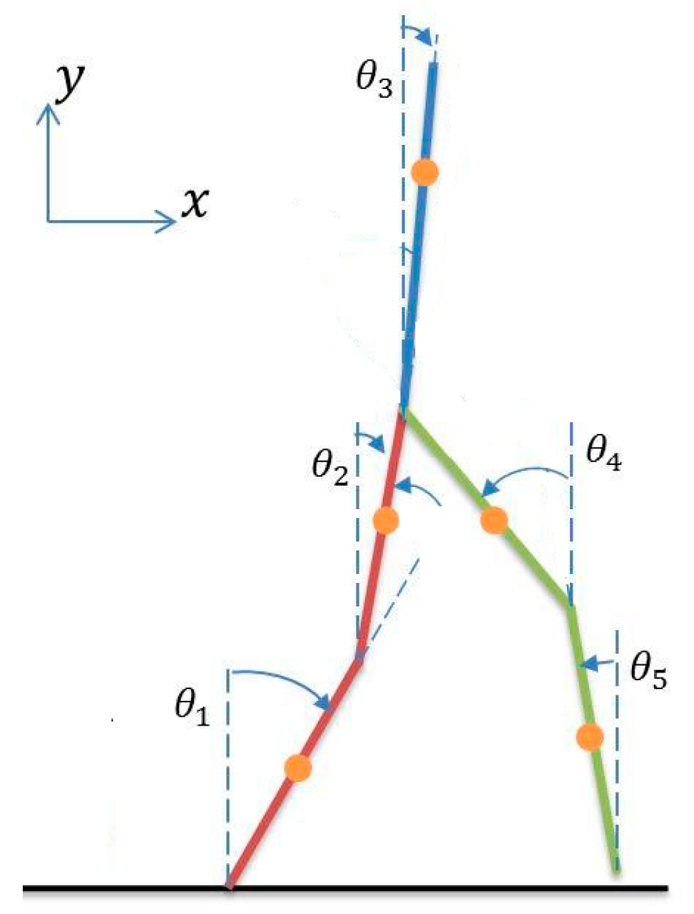
The equations of the robot are in the form below, according to the angle values shown in Figure 4.

$$\overrightarrow{\theta }={\left[\begin{array}{ccccc}{\theta }_1& {\theta }_2& {\theta }_3& {\theta }_4& {\theta }_5\end{array}\right]}^T$$

(33)

$$\left[D\left(\overrightarrow{\theta }\right)\right]\overrightarrow{\ddot{\theta }}+\left[H\left(\overrightarrow{\theta },\overrightarrow{\dot{\theta }}\right)\right]\overrightarrow{\dot{\theta }}+\overrightarrow{G}\left(\overrightarrow{\theta }\right)=\overrightarrow{\tau }$$

(34)

Here, Equation (33) is a vector of size 1*5 and represents the angular positions of the joints of the biped robot according to Figure 4. $\left[D\left(\overrightarrow{\theta }\right)\right]$ is an inertia matrix of size 5*5. $\left[H\left(\overrightarrow{\theta },\overrightarrow{\dot{\theta }}\right)\right]\overrightarrow{\dot{\theta }}$ is a vector of size 1*5 and represents the centrifugal forces and Coriolis accelerations. $\overrightarrow{G}\left(\overrightarrow{\theta }\right)$ is the gravitational force vector and $\overrightarrow{\tau }$ is the vector related to the input control moments. These parameters will be defined in the following sections according to [29].

$$\left[D\left(\overrightarrow{\theta }\right)\right]=\left[\begin{array}{ccccc}{p}_{11}& p_{12}\mathit{cos}\left({\theta }_1-{\theta }_2\right)& p_{13}\mathit{cos}\left({\theta }_1-{\theta }_3\right)& p_{14}\mathit{cos}\left({\theta }_1+{\theta }_4\right)& p_{15}\mathit{cos}\left({\theta }_1+{\theta }_5\right)\\ p_{12}\mathit{cos}\left({\theta }_1-{\theta }_2\right)& p_{22}& p_{23}\mathit{cos}\left({\theta }_2-{\theta }_3\right)& p_{24}\mathit{cos}\left({\theta }_2+{\theta }_4\right)& p_{25}\mathit{cos}\left({\theta }_2+{\theta }_5\right)\\ p_{13}\mathit{cos}\left({\theta }_1-{\theta }_3\right)& p_{23}\mathit{cos}\left({\theta }_2-{\theta }_3\right)& p_{33}& 0& 0\\ p_{14}\mathit{cos}\left({\theta }_1+{\theta }_4\right)& p_{24}\mathit{cos}\left({\theta }_2+{\theta }_4\right)& 0& p_{44}& p_{45}\mathit{cos}\left({\theta }_4-{\theta }_5\right)\\ p_{15}\mathit{cos}\left({\theta }_1+{\theta }_5\right)& p_{25}\mathit{cos}\left({\theta }_2+{\theta }_5\right)& 0& p_{45}\mathit{cos}\left({\theta }_4-{\theta }_5\right)& p_{55}\end{array}\right]$$

(35)

$$\left[H\left(\overrightarrow{\theta },\overrightarrow{\dot{\theta }}\right)\right]=\left[\begin{array}{ccccc}0& p_{12}\mathit{sin}\left({\theta }_1-{\theta }_2\right){\dot{\theta }}_2& p_{13}\mathit{sin}\left({\theta }_1-{\theta }_3\right){\dot{\theta }}_3& -p_{14}\mathit{sin}\left({\theta }_1+{\theta }_4\right){\dot{\theta }}_4& -p_{15}\mathit{sin}\left({\theta }_1+{\theta }_5\right){\dot{\theta }}_5\\ -p_{12}\mathit{sin}\left({\theta }_1-{\theta }_2\right){\dot{\theta }}_1& 0& p_{23}\mathit{sin}\left({\theta }_2-{\theta }_3\right){\dot{\theta }}_3& -p_{24}\mathit{sin}\left({\theta }_2+{\theta }_4\right){\dot{\theta }}_4& -p_{25}\mathit{sin}\left({\theta }_2+{\theta }_5\right){\dot{\theta }}_5\\ -p_{13}\mathit{sin}\left({\theta }_1-{\theta }_3\right){\dot{\theta }}_1& -p_{23}\mathit{sin}\left({\theta }_2-{\theta }_3\right){\dot{\theta }}_2& 0& 0& 0\\ -p_{14}\mathit{sin}\left({\theta }_1+{\theta }_4\right){\dot{\theta }}_1& -p_{24}\mathit{sin}\left({\theta }_2+{\theta }_4\right){\dot{\theta }}_2& 0& 0& p_{45}\mathit{cos}\left({\theta }_4-{\theta }_5\right){\dot{\theta }}_5\\ -p_{15}\mathit{sin}\left({\theta }_1+{\theta }_5\right){\dot{\theta }}_1& -p_{25}\mathit{sin}\left({\theta }_2+{\theta }_5\right){\dot{\theta }}_2& 0& -p_{45}\mathit{sin}\left({\theta }_4-{\theta }_5\right){\dot{\theta }}_4& 0\end{array}\right]$$

(36)

$$\overrightarrow{G}=g\left[\begin{array}{c}-q_1\mathit{sin}\left({\theta }_1\right)\\ -q_2\mathit{sin}\left({\theta }_2\right)\\ -q_3\mathit{sin}\left({\theta }_3\right)\\ q_4\mathit{sin}\left({\theta }_4\right)\\ q_5\mathit{sin}\left({\theta }_5\right)\end{array}\right]$$

(37)

$p_{11},p_{12},p_{13},p_{14},p_{15},p_{22},p_{23},p_{24},p_{25},p_{33},p_{44},p_{45},p_{55},q_1,q_2,q_3,q_4, \mathrm{a}\mathrm{n}\mathrm{d} q_5$ are constants in the equations of motion and depend on the fixed parameters of the robot.

$$\begin{array}{c}{p}_{11}=I_1+m_1{d}_1^2+\left(m_2+m_3+m_4+m_5\right)l_1^2\\ p_{12}=m_2{d}_2{l}_1+\left(m_3+m_4+m_5\right)l_1{l}_2\\ p_{13}=m_3{d}_3{l}_1\\ p_{14}=m_4{l}_1\left(l_4-d_4\right)+m_5{l}_1{l}_4\\ p_{15}=m_5{l}_1\left(l_5-d_5\right)\\ p_{22}=I_2+m_2{d}_2^2+\left(m_3+m_4+m_5\right)l_2^2\\ p_{23}=m_3{l}_2{d}_3\\ p_{24}=m_4{l}_2\left(l_4-d_4\right)+m_5{l}_2{l}_4\\ p_{25}=m_5{l}_2\left(l_5-d_5\right)\\ p_{33}=I_3+m_3{d}_3^2\\ p_{44}=I_4+m_4{\left(l_4-d_4\right)}^2+m_5{l}_4^2\\ p_{45}=m_5{l}_4\left(l_5-d_5\right)\\ p_{55}=I_5+m_5\left(l_5-d_5\right)\\ q_1=m_1{d}_1+\left(m_2+m_3+m_4+m_5\right)l_1\\ q_2=m_2{d}_2+\left(m_3+m_4+m_5\right)l_2\\ q_3=m_3{d}_3\\ q_4=m_4\left(l_4-d_4\right)+m_5{l}_4\\ q_5=m_5\left(l_5-d_5\right)\end{array}$$

(38)

m₁, m₂, m₃, m₄, and m₅ are the masses of links 1 through 5. l₁, l₂, l₃, l₄, and l₅ are the lengths of links 1 through 5. I₁, I₂, I₃, I₄, and I₅ are the moments of inertia of links 1 through 5. d₁, d₂, d₃, d₄, and d₅ are the centers of mass of links 1 through 5.

In [28], as the basis for controller design for the robot, the control vector equation for nominal values (the case where the fixed parameters of the robot are known exactly) is defined as follows:

$${\overrightarrow{\tau }}_0=\left[D\left(\overrightarrow{\theta }\right)\right]\overrightarrow{a}+\left[H\left(\overrightarrow{\theta },\overrightarrow{\dot{\theta }}\right)\right]\overrightarrow{v}+\overrightarrow{G}\left(\overrightarrow{\theta }\right)-\left[K_D\right]\overrightarrow{r}$$

(39)

$$\begin{array}{c}\overrightarrow{v}={\overrightarrow{\dot{\theta }}}_d-\left[\mathsf{\Lambda }\right]\overrightarrow{\tilde{\theta }}\\ \overrightarrow{a}=\overrightarrow{\dot{v}}\\ r=\overrightarrow{\dot{\tilde{\theta }}}+\left[\mathsf{\Lambda }\right]\overrightarrow{\tilde{\theta }}\\ \overrightarrow{\tilde{\theta }}=\overrightarrow{\theta }-{\overrightarrow{\theta }}_d\end{array}$$

(40)

$\left[\mathsf{\Lambda }\right]$ and $\left[K_D\right]$ are constant diagonal matrices with positive members. Equation (39) is obtained by the Lyapunov stability method. In fact, this equation is the result of previous research of the authors of the reference paper and is discussed in detail in reference [28]. In practice, it is not possible to specify an exact value for the fixed parameters of the robot (m_i, l_i, d_i, and I_i). For example, the robot may move objects whose mass or inertia parameters are uncertain, or the link lengths of the robot may change due to elastic effects. Adaptive control is a method for controlling such systems. The basic idea of adaptive control is to estimate the uncertain parameters based on measured signals and use these estimated parameters in control input calculations.

$${\overrightarrow{\tau }}_0=\left[Y\left(\overrightarrow{\theta },\overrightarrow{\dot{\theta }},\overrightarrow{v},\overrightarrow{a}\right)\right]\overrightarrow{\Theta }-\left[K_D\right]\overrightarrow{r}$$

(41)

In the reference paper, the controller introduced in Equation (39) is formulated in Equation (42) based on fixed parameters (which are uncertain).

$$\left[D\left(\overrightarrow{\theta }\right)\right]\overrightarrow{a}+\left[H\left(\overrightarrow{\theta },\overrightarrow{\dot{\theta }}\right)\right]\overrightarrow{v}+\overrightarrow{G}\left(\overrightarrow{\theta }\right)=\left[Y\left(\overrightarrow{\theta },\overrightarrow{\dot{\theta }},\overrightarrow{v},\overrightarrow{a}\right)\right]\overrightarrow{\Theta }$$

(42)

$\overrightarrow{\Theta }$ vector are non-repeating constants that appear in the equations and whose value is the same as the constant parameters $p_{11},\dots ,p_{55},q_1,\dots ,q_5$.

As noted, the value of $\overrightarrow{\Theta }$ is practically unknown. In the reference article [28], the difference between the nominal and real values of $\overrightarrow{\Theta }$ is assumed to be of the following form:

$\rho$ is a limited and positive value. In the reference [28] used for controller design, the uncertain values $\overrightarrow{\Theta }$ are expressed in Equation (43).

$$\overrightarrow{\tau }={\overrightarrow{\tau }}_0+\left[Y\left(\overrightarrow{\theta },\overrightarrow{\dot{\theta }},\overrightarrow{v},\overrightarrow{a}\right)\right]u=\left[Y\left(\overrightarrow{\theta },\overrightarrow{\dot{\theta }},\overrightarrow{v},\overrightarrow{a}\right)\right]\left({\overrightarrow{\Theta }}_0+u\right)-\left[K_D\right]\overrightarrow{r}$$

(43)

Here u;

$$u=\left\{\begin{array}{l}-\widehat{\rho }{\displaystyle \frac{{\left[Y\right]}^T\overrightarrow{r}}{‖{\left[Y\right]}^T\overrightarrow{r}‖}}‖\widehat{\rho }{\left[Y\right]}^T\overrightarrow{r}‖>\epsilon \\ -{{\displaystyle \frac{\widehat{\rho }}{\epsilon }}}^2{\left[Y\right]}^T\overrightarrow{r}‖\widehat{\rho }{\left[Y\right]}^T\overrightarrow{r}‖\le \epsilon \end{array}\right.$$

(44)

$$\left\{\begin{array}{l}\dot{\widehat{\rho }}=L‖{\left[Y\right]}^T\overrightarrow{r}‖\\ \dot{\epsilon }=-l\epsilon \end{array}\right.$$

(45)

$\widehat{\rho }$ is the estimation of $\rho$. L and I are constant.

Proof. 

The proof of global convergence is based on showing that the function [28]

$$V={\displaystyle \frac{1}{2}}{r}^{T}M\left(q\right)r+{\tilde{q}}^T{\Lambda }^T{K}_D\tilde{q}+{\displaystyle \frac{1}{2}}{\left(\tilde{\rho }-\rho \right)}^T{L}^{-1}\left(\tilde{\rho }-\rho \right)+{\displaystyle \frac{\epsilon }{l}}$$

(46)

is a Lyapunov function for the closed-loop system. Here, M is a skew-symmetric matrix. The derivative of the Lyapunov function is;

$$\dot{V}=-x^{T}Qx+w^T\left\{\tilde{\theta }+u\right\}+\left(\widehat{\rho }-\rho \right)‖w‖-\epsilon$$

(47)

where

$$x^T=\left[{\tilde{q}}^T,{\dot{\tilde{q}}}^T\right], w=Y^{T}r\mathrm{and} Q=diag\left\{{\Lambda }^T{K}_D\Lambda ,K_D\right\}$$

(48)

Note that Q is positive definite, making the first term in (48) negative semi-definite. □

Case 1. 

If $‖w‖>{\displaystyle \raisebox{1ex}{$\epsilon $}\!\left/ \!\raisebox{-1ex}{$\widehat{\rho }$}\right.}$ then  $u=-\widehat{\rho }w/‖w‖$  and we have;

$$\begin{array}{c}{w}^T\left\{\tilde{\theta }+u\right\}+\left(\widehat{\rho }-\rho \right)‖w‖-\epsilon =w^T\tilde{\theta }-\rho ‖w‖-\epsilon \\ \le ‖w‖\left\{‖\tilde{\theta }‖-\rho \right\}-\epsilon \\ \le 0\end{array}$$

(49)

from the Cauchy-Schwartz inequality and our assumption on $‖\tilde{\theta }‖$.

Case 2. 

If $‖w‖\le {\displaystyle \raisebox{1ex}{$\epsilon $}\!\left/ \!\raisebox{-1ex}{$\widehat{\rho }$}\right.}$ then  $u=-{\widehat{\rho }}^2/\epsilon$  and we have;

$$\begin{array}{c}{w}^T\left\{\tilde{\theta }+u\right\}+\left(\widehat{\rho }-\rho \right)‖w‖-\epsilon =w^T\tilde{\theta }-{\displaystyle \frac{{\widehat{\rho }}^2}{\epsilon }}{‖w‖}^2+\widehat{\rho }‖w‖-\rho ‖w‖-\epsilon \\ \le ‖w‖\left\{‖\tilde{\theta }‖-\rho \right\}-{\displaystyle \frac{{\widehat{\rho }}^2}{\epsilon }}{‖w‖}^2+\left\{\widehat{\rho }‖w‖+\epsilon \right\}\\ \le 0\end{array}$$

(50)

Since  $‖\tilde{\theta }‖\le \rho$  and  $‖w‖\le {\displaystyle \raisebox{1ex}{$\epsilon $}\!\left/ \!\raisebox{-1ex}{$\widehat{\rho }$}\right.}$. Therefore, we have shown that

$$\dot{V}\le -xQx$$

(51)

3. Results

The modeling of a two-legged robot can be divided into three parts: linkages, actuators, and the contact surface model. Three subsystems can be defined: both legs and the torso, and an input signal generated by an external controller that allows torque to be applied to each actuator. The values used for the modeling were determined for the simulation of an adult person weighing 75 kg and standing 1.70 m tall. The values of the leg and body are given in

Table A1. The value of a parameter belonging to the body.

Mass	c (m)	b (m)	a (m)
35	0.4	0.7	0.15

and

Table A2. The value of a parameter belonging to the leg.

Mass	R (m)	h (m)
8.75	0.15	0.7

in Appendix A.

In this section, a detailed analysis of simulation results for adaptive control of a bipedal robot with 5 degrees of freedom (DOF) is presented. Each joint angle is analyzed from θ₁ to θ₅, and the shapes are explained using important inferences from Spong’s adaptive control theory. The simulations were performed in MATLAB/Simulink using a fixed-step Runge–Kutta solver. To ensure numerical stability and achieve accurate results, the integration step size was set to 0.001 s. Control parameters were obtained by trial and error. Numerous trials were conducted until optimum results were obtained.

3.1. Trajectory Tracking for θ₁ (Hip Joint)

Figure 5 shows the tracking performance and tracking error of the adaptive controller in tracking the robot’s hip joint θ₁. The adaptive controller showed minimum deviation by following the desired trajectory with high precision throughout the simulation. This precision can be attributed to the passive-based adaptive control law that updates the control law in real time based on the tracking error. The solid blue line represents the actual trajectory of the hip joint angle under the proposed adaptive control strategy, while the dashed line indicates the desired reference trajectory. As shown in the figure, the controlled joint angle converges to the desired position within approximately 1 to 1.5 s, demonstrating a fast and stable response. The error plot further confirms that the system maintains a very small deviation from the desired trajectory, indicating high tracking accuracy.

As Spong [28] points out, the controller can dynamically adjust torque inputs due to the linearity of robot dynamics with parameters. While the nominal control law τ0 is designed based on fixed system parameters, additional control inputs compensate for uncertainties. This results in accurate tracking even in the presence of unmodeled dynamics. The adaptive controller effectively minimizes tracking error by adjusting control inputs in real time based on Spong’s proposed Lyapunov function stability criterion. This enables the controller to exhibit robust tracking performance even under parameter uncertainties.

3.2. Trajectory Tracking for θ₂ (Knee Joint)

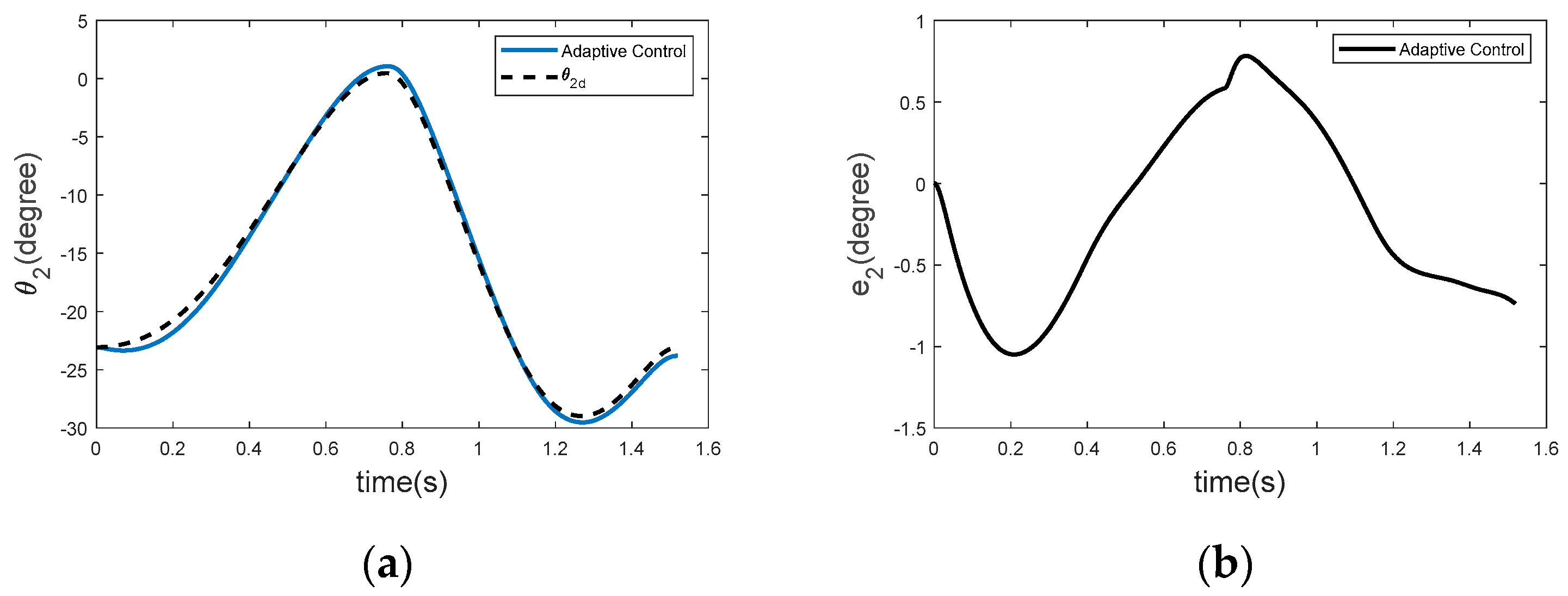
Figure 6 shows the tracking performance for the knee joint θ₂. The adaptive controller manages to stay close to the desired trajectory despite the more complex dynamics at the knee joint. According to Spong’s formulation [28], the adaptive control law guarantees stability by adjusting only two key parameters regardless of the number of links. This reduces the complexity of the control system while maintaining robustness. The controller dynamically adjusts the torque inputs to minimize the error and enables the system to respond quickly to perturbations or changes in joint dynamics. The adaptive controller is extremely effective in dealing with the complex dynamics of the knee joint. It quickly compensates for deviations, ensuring that the tracking error remains limited. This robust performance is one of the key features of the passive-based control approach.

3.3. Trajectory Tracking for θ₃ (Ankle Joint)

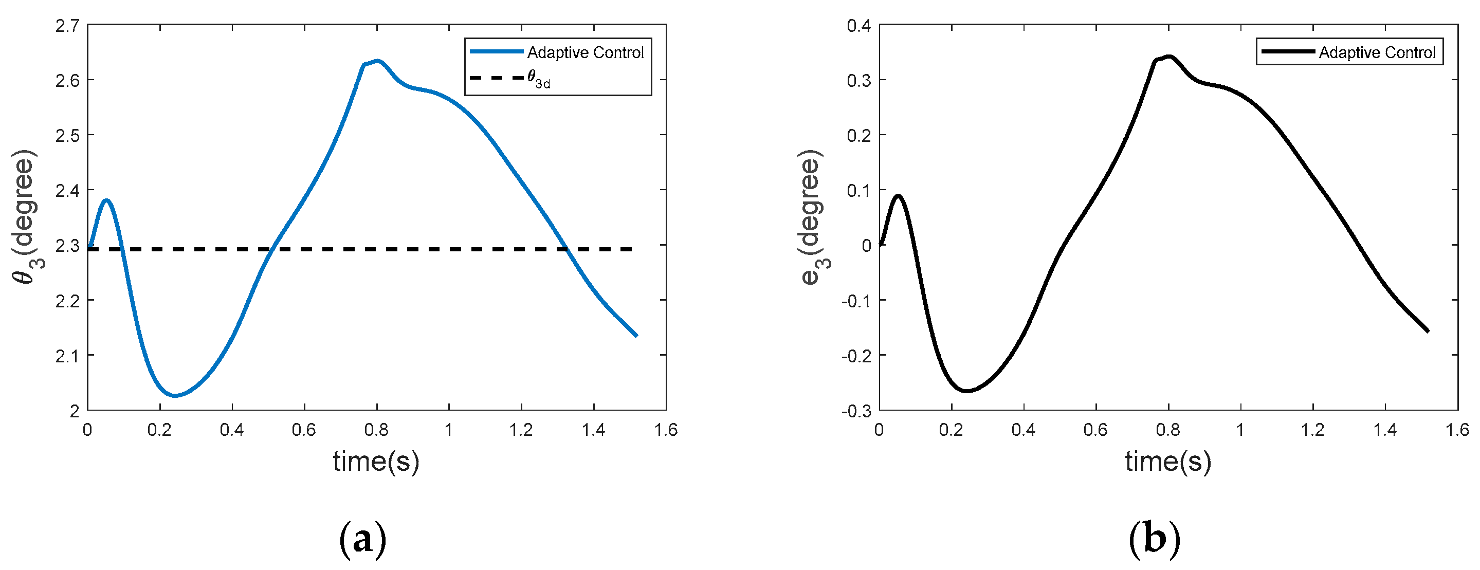
Figure 7 shows the response of the ankle joint θ₃ under adaptive control. Since the ankle is subjected to higher impact forces and rapid dynamic changes during walking, slightly larger deflections are observed compared to other joints. However, the adaptive controller still performs well by rapidly decreasing the error after the transient stages. Spong’s control law [28] includes an update term u to handle such dynamic changes. By avoiding unnecessary parameter updates, the probability of the system experiencing parameter drift or instability is reduced. This allows the system to maintain robust performance even in joints such as the ankle that experience rapid dynamic changes. Larger deflections at the ankle joint are quickly corrected by the adaptive controller, reflecting the controller’s capabilities in handling rapid dynamic changes. A control design that reduces the number of parameter updates required increases efficiency by maintaining stability.

3.4. Trajectory Tracking for θ₄ (Lower Limb Joint)

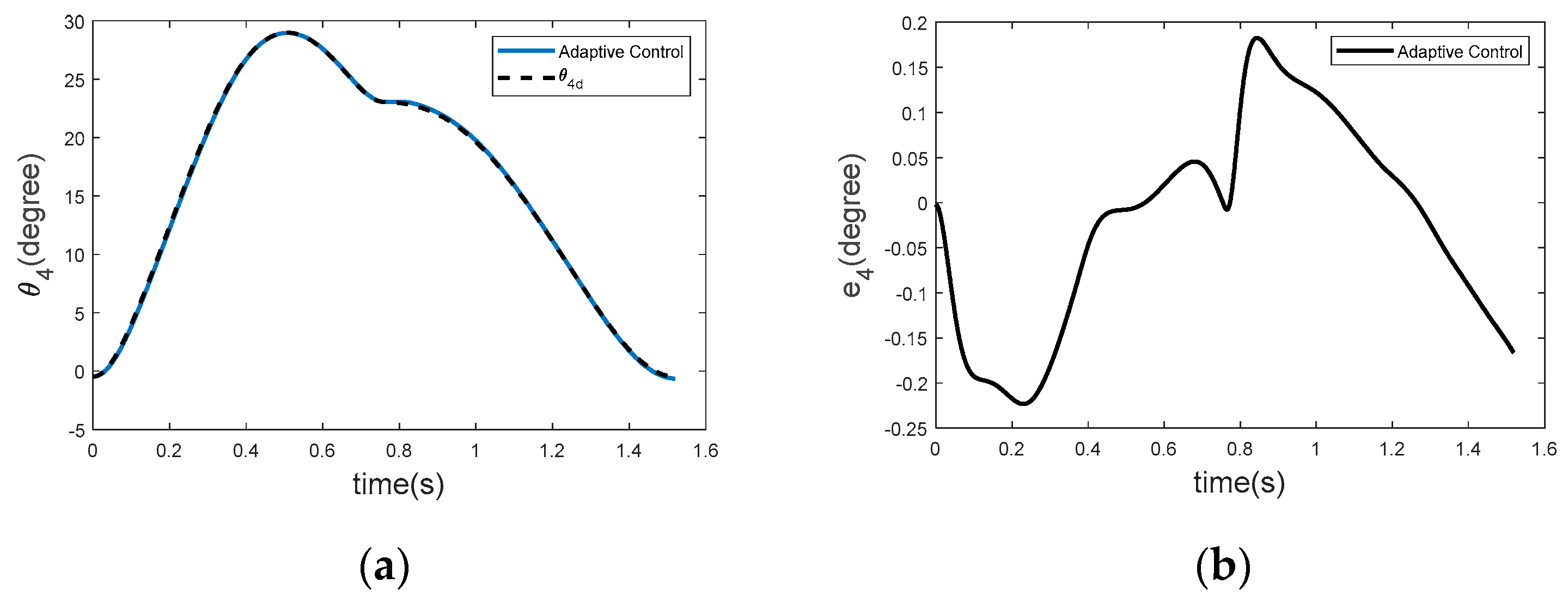
Figure 8 illustrates the performance of the adaptive controller for the lower limb joint θ₄. The controller demonstrates strong tracking accuracy and effective error minimization. It achieves the desired trajectory more rapidly and maintains a lower steady-state error compared to conventional methods. Spong’s adaptive control approach [28], grounded in the Lyapunov stability criterion, guarantees that all system signals remain bounded and that the tracking error asymptotically converges to zero. This stability criterion ensures reliable system performance even in the presence of unmodeled dynamics.

3.5. Trajectory Tracking for θ₅ (Upper/Lower Limb Joint)

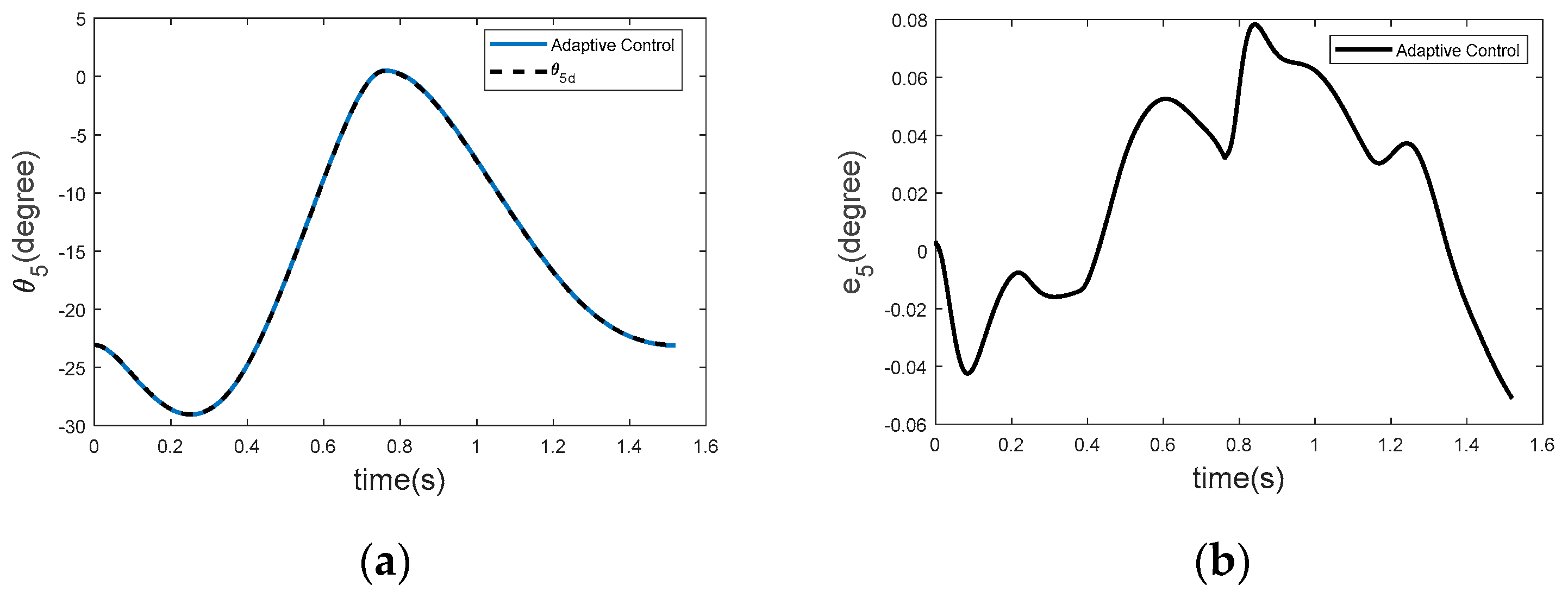
Figure 9 presents an analysis of the steady-state error for the θ₅ joint. The adaptive controller rapidly reduces the tracking error to near zero, demonstrating its capability to maintain long-term accuracy after transient effects have subsided. Spong’s adaptive control method [28] mitigates the risk of parameter drift by limiting the frequency of parameter updates, thereby ensuring consistent performance. Utilizing the Lyapunov stability framework, the system converges to a steady state with minimal trajectory tracking error. The adaptive controller’s effective reduction of steady-state error makes it a suitable choice for applications demanding sustained precision. Furthermore, the robustness of the controller in preserving accuracy over extended periods underscores the advantages of the passivity-based adaptive control approach.

Figure 10 illustrates the torque forces generated by the adaptive controller when applied to the biped robot. These torques correspond to the following joints: hip joint (θ₁), knee joint (θ₂), ankle joint (θ₃), lower limb joint (θ₄), and upper/lower limb connecting joint (θ₅). The torque profiles represent the control effort required at each joint to maintain balance and follow the desired motion trajectories. The adaptive controller continuously adjusts these torques in real time based on the robot’s dynamic behavior and feedback, ensuring stability and robustness against uncertainties or external disturbances. The initial phase of the simulation shows all joints producing positive torques, indicating an initial effort to initiate movement and maintain postural balance. The hip (θ₁) and knee (θ₂) joints exhibit the highest torque values, exceeding 600 N. This suggests that these joints are primarily responsible for generating the required propulsion and managing the robot’s center of mass during the initial stance.

In the intermediate phase, there is a noticeable decline in torque values at θ₁ and θ₂, both transitioning to significant negative levels. This behavior is indicative of a counter-torque phase, possibly during the swing or mid-stance, where the robot adjusts its posture or prepares for the next step. Meanwhile, joints such as the lower limb (θ₃) and the upper limb joint (θ₅) exhibit relatively minor fluctuations, pointing to their more supportive or compensatory roles.

In the final phase, torque values rise again, especially at θ₁ and θ₂, demonstrating a reapplication of force likely associated with the completion of the step and preparation for the next gait cycle. The adaptive controller’s ability to manage such transitions without instability indicates its robustness and responsiveness.

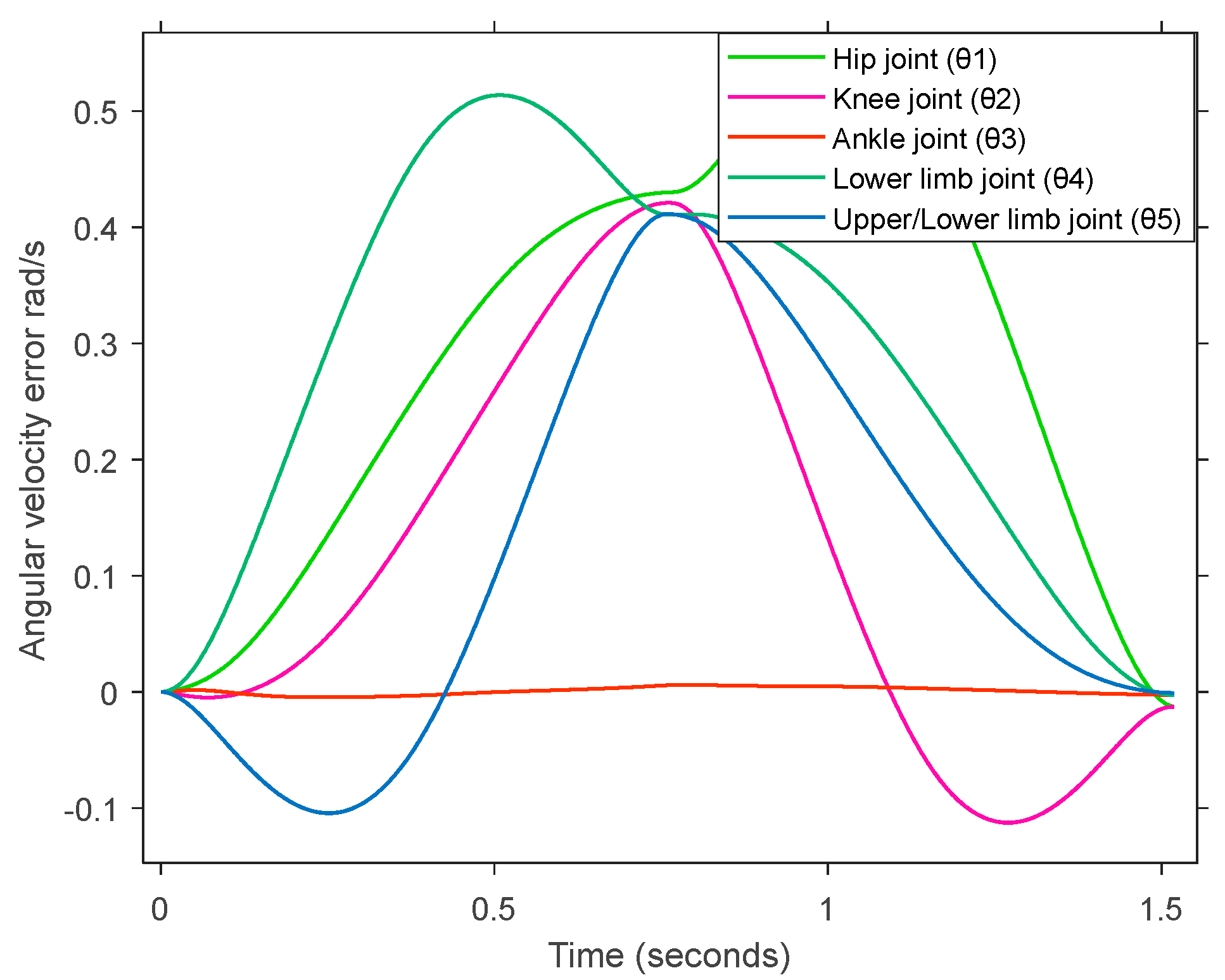
Figure 11 presents the angular velocity error profiles of five joints in the biped robot over time. The plotted data correspond to the following joints: hip joint (θ₁), knee joint (θ₂), ankle joint (θ₃), lower limb joint (θ₄), and upper/lower limb joint (θ₅). All joint velocity errors exhibit a transient bell-shaped behavior, with error values starting near zero, returning to zero by t = 1.5 s. This trend reflects the controller’s response to dynamic motion demands during a single gait cycle and indicates symmetrical error behavior in most joints. The hip joint (θ₁) and lower limb joint (θ₄) exhibit the largest error magnitudes, reaching values above 0.5 rad/s. These joints likely undergo significant load variation and play a critical role in maintaining balance and forward motion. The knee joint (θ₂) and upper/lower limb joint (θ₅) present moderate error levels, with peak values around 0.4 rad/s. The ankle joint (θ₃) shows minimal error, remaining within the narrow range of ±0.05 rad/s, suggesting excellent velocity tracking performance for that joint.

While larger joints such as the hip and lower limb exhibit higher errors due to dynamic demands, the controller ensures all joints converge to zero error over time. This indicates strong adaptability, stability, and precision in joint-level control, which is essential for maintaining balance and achieving smooth locomotion in biped robots.

4. Discussion

The results presented in Figure 5, Figure 6, Figure 7, Figure 8 and Figure 9 clearly demonstrate that the adaptive controller outperforms alternative approaches in terms of trajectory tracking, error minimization, and robustness. Its ability to adjust control inputs in real time based on feedback allows for effective management of system uncertainties and external disturbances. By leveraging Spong’s passivity-based adaptive control framework, the system achieves superior performance while maintaining low computational complexity. The robustness, efficiency, and precision of the adaptive controller make it a highly effective solution for managing the complex dynamics of a 5-DOF bipedal robot.

5. Conclusions

In this study, an adaptive control system based on a five-degree-of-freedom (DOF) model of a bipedal robot was investigated in the context of robotic motion control. The primary objective was to optimize control performance in the presence of uncertainties in the system’s dynamic parameters. The simulation results and corresponding analyses demonstrate the effectiveness and accuracy of the proposed adaptive control approach.

The key advantage of the adaptive control system lies in its ability to identify uncertainties in system parameters in real time and dynamically adjust its control strategy accordingly. Unlike conventional control methods, the adaptive controller compensates for uncertain parameters such as variations in the robot’s mass, joint friction, and inertia. As a result, high tracking accuracy is achieved without compromising control performance, even under varying system conditions. The most significant feature of the proposed controller is its model-independence, allowing for broad applicability across different systems. Additionally, its adaptive nature ensures effective performance in the presence of external disturbances and uncertainties.

In robotic systems, particularly in bipedal robots, it is common for dynamic parameters to vary continuously due to external factors such as ground reaction forces, gravitational effects, and abrupt changes in motion direction. These variations result in instantaneous changes in the load on the robot’s joints. The adaptive control system demonstrates robust performance under such dynamic uncertainties, effectively maintaining overall system stability.

The tracking results for joint angles θ₃ (ankle joint) and θ₄, as presented in Figure 7 and Figure 8, indicate that the adaptive controller adapts rapidly and effectively to dynamic changes. Based on control principles developed by Spong, the system optimizes control inputs with minimal parameter updates, ensuring stable operation even in joints exposed to rapid motion and external disturbances. Notably, the tracking error at the ankle joint remains consistently low, despite being subjected to significant dynamic loads.

Steady-state performance is another critical metric for evaluating the long-term effectiveness of a control strategy. As shown in Figure 9 and subsequent figures, the adaptive controller maintains high accuracy by minimizing the steady-state error over time. Using the Lyapunov stability criterion, the adaptive control system asymptotically reduces the tracking error to zero. The passivity-based control approach introduced by Spong ensures the boundedness of all system signals while minimizing control errors. Remarkably, the steady-state error for the θ₅ joint approaches zero, indicating the controller’s optimal performance for that joint.

Furthermore, transient behavior is a key indicator of how effectively a control system responds to rapid dynamic changes. The tracking error results demonstrate that the adaptive controller reacts promptly during transient phases, significantly reducing the error within a short time frame. After initial deviations, the system quickly converges to the desired trajectory, showcasing the controller’s strong error correction capabilities. This responsiveness is particularly important in scenarios where the robot temporarily loses balance; in such cases, the adaptive controller rapidly intervenes to restore system stability—a critically important feature for highly dynamic systems such as bipedal robots.

Future research could explore the use of alternative control strategies, including dual control, for managing the proposed model. For example, ref. [30] introduced the dual control for exploration and exploitation (DCEE) algorithm, which is based on the Nesterov accelerated gradient descent (NAGD). This approach aims to achieve an optimal balance between operational performance and learning. The convergence of both source term estimation and path planning in the DCEE-NAGD framework was rigorously established using the mean value theorem and mathematical transformations, thereby ensuring optimal stability. Given its novelty and effectiveness, this control law holds potential for application in bipedal robot systems, where its performance could be further investigated and compared.