Project Report

On Control Synthesis of Hydraulic Servomechanisms in Flight Controls Applications

National Institute for Aerospace Research Elie Carafoli—INCAS, Blvd. Iuliu Maniu 220, 061126 Bucharest, Romania
*
Author to whom correspondence should be addressed.
Actuators 2025, 14(7), 346; https://doi.org/10.3390/act14070346
Submission received: 30 May 2025 / Revised: 7 July 2025 / Accepted: 8 July 2025 / Published: 14 July 2025
(This article belongs to the Special Issue Advanced Technologies in Actuators for Control Systems)

Abstract

This paper presents some of the most significant findings in the design of a hydraulic servomechanism for flight controls, which were primarily achieved by the first author during his activity in an aviation institute. These results are grouped into four main topics. The first one outlines a classical theory, from the 1950s–1970s, of the analysis of nonlinear automatic systems and namely the issue of absolute stability. The uninformed public may be misled by the adjective “absolute”. This is not a “maximalist” solution of stability but rather highlights in the system of equations a nonlinear function that describes, for the case of hydraulic servomechanisms, the flow-control dependence in the distributor spool. This function is odd, and it is therefore located in quadrants 1 and 3. The decision regarding stability is made within the so-called Lurie problem and is materialized by a matrix inequality, called the Lefschetz condition, which must be satisfied by the parameters of the electrohydraulic servomechanism and also by the components of the control feedback vector. Another approach starts from a classical theorem of V. M. Popov, extended in a stochastic framework by T. Morozan and I. Ursu, which ends with the description of the local and global spool valve flow-control characteristics that ensure stability in the large with respect to bounded perturbations for the mechano-hydraulic servomechanism. We add that a conjecture regarding the more pronounced flexibility of mathematical models in relation to mathematical instruments (theories) was used. Furthermore, the second topic concerns, the importance of the impedance characteristic of the mechano-hydraulic servomechanism in preventing flutter of the flight controls is emphasized. Impedance, also called dynamic stiffness, is defined as the ratio, in a dynamic regime, between the output exerted force (at the actuator rod of the servomechanism) and the displacement induced by this force under the assumption of a blocked input. It is demonstrated in the paper that there are two forms of the impedance function: one that favors the appearance of flutter and another that allows for flutter damping. It is interesting to note that these theoretical considerations were established in the institute’s reports some time before their introduction in the Aviation Regulation AvP.970. However, it was precisely the absence of the impedance criterion in the regulation at the appropriate time that ultimately led, by chance or not, to a disaster: the crash of a prototype due to tailplane flutter. A third topic shows how an important problem in the theory of automatic systems of the 1970s–1980s, namely the robust synthesis of the servomechanism, is formulated, applied and solved in the case of an electrohydraulic servomechanism. In general, the solution of a robust servomechanism problem consists of two distinct components: a servo-compensator, in fact an internal model of the exogenous dynamics, and a stabilizing compensator. These components are adapted in the case of an electrohydraulic servomechanism. In addition to the classical case mentioned above, a synthesis problem of an anti-windup (anti-saturation) compensator is formulated and solved. The fourth topic, and the last one presented in detail, is the synthesis of a fuzzy supervised neurocontrol (FSNC) for the position tracking of an electrohydraulic servomechanism, with experimental validation, in the laboratory, of this control law. The neurocontrol module is designed using a single-layered perceptron architecture. Neurocontrol is in principle optimal, but it is not free from saturation. To this end, in order to counteract saturation, a Mamdani-type fuzzy logic was developed, which takes control when neurocontrol has saturated. It returns to neurocontrol when it returns to normal, respectively, when saturation is eliminated. What distinguishes this FSNC law is its simplicity and efficiency and especially the fact that against quite a few opponents in the field, it still works very well on quite complicated physical systems. Finally, a brief section reviews some recent works by the authors, in which current approaches to hydraulic servomechanisms are presented: the backstepping control synthesis technique, input delay treated with Lyapunov–Krasovskii functionals, and critical stability treated with Lyapunov–Malkin theory.

1. Introduction

This paper presents some of the most insightful results obtained by the first author during his activity in an aerospace research and design institute, in the field of analysis, synthesis, qualification and flight clearance of hydraulic servomechanisms used in aircraft and helicopters [1]. The publications [2,3,4,5] are bibliographic sources for the detailed presentation in Section 2, Section 3, Section 4 and Section 5 of some representative contributions regarding hydraulic servomechanism projects. It is worth mentioning that the paper [4] received an award of excellence from the journal in which it was published. Additional results of the authors are summarized in Section 6. Also, some recent results from the literature regarding the synthesis of hydraulic servomechanisms are presented.
First, we outline some of the lessons learned concerning the philosophy of research in the field of automatic systems synthesis.
Starting from extensive experience in mathematical modeling and working with mathematical instruments (MI) for control synthesis, the following strategy has been outlined for handling mathematical models (MMs) and MI: (a) the derivation of an MM as complex as possible, ensuring alignment with the physical laws and constraints that define the physical model (PHM); (b) adjustment and simplification of the MM to meet the rigor required by the MI used in system design and analysis; (c) providing a controlled systems design and optimized solution; (d) iterative validation of the solution through numerical simulations on the complex MM, followed by experimental tests on a PHM and, finally, on a physical object (PHO) as a controlled system (CS). For a certain chosen PHM, multiple MMs can be formulated through successive fitting, completion or reduction in the initial MIs. Thus, our empirical insights focus on the behavior of MMs in connection with MIs of control synthesis [6,7]:
Lesson 1.
All MMs, describing the same object ultimately exhibit a degree of consistency and coherence, meaning they will predict similar CS performance or behavior improvement regardless of the mathematical MI of control synthesis used.
Lesson 2.
An MM, as a first product of thinking, derived from a physical reality, is more “flexible” than an MI (i.e., a mathematical theory, which is a second-order product of thinking, derived from a meta-reality, here, mathematical thinking).
Thus, the first lesson highlights certain conservative properties of MMs. The second conjecture advances a compensating property of MMs. This is a complemental, flexibility property: to be able to apply a certain mathematical construction, a mathematical model can be often “shaped” in view of coping with the constraints of a certain mathematical apparatus (see the example within this section).
To further emphasize the significance of these statements, a quote from the renowned work of K. J. Popper [8] presents the principle of falsifiability as a criterion for distinguishing between science and pseudoscience: “I do not claim that every statement should be tested in fact, only that every statement should be testable; or, in other words, I refuse to accept the view that there are statements in science that must be accepted simply because it is not logically possible to test them”. In essence, MMs are basically hypotheses, which may or may not work, depending on their corroboration with certain MIs.
A third lesson concerns classical control versus the new paradigm of intelligent control. Both approaches have certainly their place in control systems theory, yet it is noteworthy that over 90% of implemented solutions still begin with PID control [9]. This trend is particularly striking given that control theory has existed for more than eight decades and has so many remarkable achievements such as LQR and LQG control along with remarkable developments in the nonlinear field. As for intelligent control, based on neural networks, fuzzy logic, genetic algorithms, and expert systems, its application may not always be justified for certain problems. Intelligent control systems excel, however, in areas that are highly nonlinear, where classical control systems fail, or when obtaining a precise model of the system is challenging or impossible.
Lesson 3.
The essential part of the intelligent control paradigm is carried out as a free model vision; thus, the control synthesis is free of a few fundamental limitations, such as linearity, time invariance, accurate mathematical representation of plants, etc.
The conclusion drawn from various approaches [10,11,12,13,14,15,16], regarding applications in active and semiactive vehicle suspensions, ABS systems, and electrohydraulic servos for primary flight controls is that intelligent control, based on neural networks and fuzzy logic, worked at least as well as classical methodologies such as PID, LQG, sliding mode control, backstepping control, etc., when comparison was possible (in the case of the thermal manikin [15], obviously a mathematical model could not be obtained, but the neuro-fuzzy control was a success).
The lessons derived from the conservativeness of the mathematical theories of classical control versus the mathematical models of the systems confirm the excessive dependency of the theory on the mathematical model over eight decades of classical control history. These findings have led the remarkable Chinese scientist Jing-Qing Han to ask rhetorically: “Control theory: Is it a theory of model or control?” [17,18]. This can explain the decrease, in last few decades, of the importance of the mathematical model in the new paradigm of modern intelligent control.

Historical Comments

Based on extensive experience in the field, the authors highlight the risk of flutter occurrence if the impedance (also called dynamic stiffness) of the mechano-hydraulic servomechanism within the flight control chain exhibits negative damping [3,19]; see Section 3. A notable historical case occurred on 24 November 1977, when an IAR 93 Eagle aircraft crashed due to tail flutter (see [20]). The negative evaluation of the aeroservoelastic compatibility of the BU-51MS hydraulic servomechanism, retrieved from decommissioned MIG-21 aircraft, had already been documented in an internal report [21]. However, decision-makers disregarded the assessment, citing the lack of specific impedance requirements in the Aviation Publication (AvP) 970 dated 1959. (Ironically, a formal impedance requirement for servomechanisms in primary flight controls was introduced a few years later in the updated version of that Regulation.) As a direct consequence of the 1977 catastrophe, the original hydraulic servomechanisms, deemed aeroservoelastically unsuitable, were replaced with new hydraulic servomechanisms manufactured in collaboration with the Dowty Group [22]. For a comprehensive understanding of the issue, it is essential to note that the stability condition outlined earlier serves only as a sufficient criterion. Failure to meet this requirement does not necessarily imply the onset of instability. Here, the relationship between certainty and the risk assessment of decisions taken at a time can be highlighted. The impedance or dynamic stiffness can also be defined for electrohydraulic servomechanisms [23].

2. The Absolute Stability of the Loaded Electrohydraulic Servomechanism

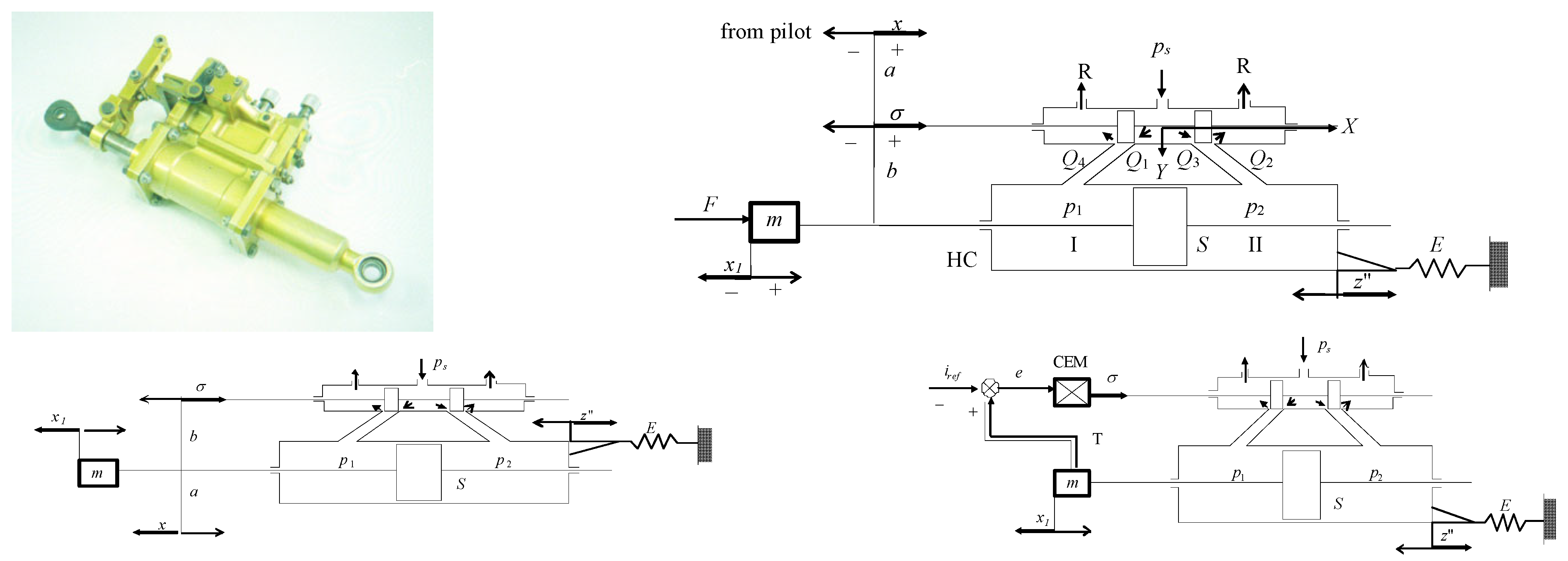
2.1. Lurie–Lefschetz Approach with Indirect Control

A recurring issue in some early literature on automatic control [24,25], concerns the canonical form of systems utilizing indirect (or derivative) control [26].
x ˙ = A x + b h ( σ ) ,   σ ˙ = c T x r h ( σ ) ,   r + c T A 1 b 0
where x ,   σ are the n-dimensional vectors representing the state variables of the plant and the control (scalar) variable, more precisely, the slot opening in the servo-valve distributor [mm], A is a constant non-singular, n × n-dimensional matrix, while b, c are n-dimensional vectors and h(σ) is the nonlinear, admissible characteristic of the actuator; finally, r is a scalar. The inequality imposes a restrictive condition on the system’s constants.
Problem 1 (Lurie’s Problem, [24,25]). 
To find necessary and sufficient conditions to have the systems (1) asymptotically stable in the large for all choices of an admissible characteristic h(σ).
This condition implies that all the solutions of the system (1) satisfy (x(t), σ (t)) → (x = 0, σ = 0) as t → ∞ indifferently of any admissible function h( σ ). In fact, the stability in the large means the stability with respect to all the state space [27]. The admissible class for h( σ ) is determined as follows: (a) h( σ ) is defined and continuous for any σ ; (b) h(0) = 0 and σh(σ) > 0, for any σ ≠ 0; (c) 0 + h ( σ ) d σ divergent (→ ∞).
The point (x = 0, σ = 0) represents a critical (singular) point of system (1). The absolute stability supposes the following: (i) there exists only one critical point; (ii) the matrix A is stable; and (iii) the inequality in (1) holds.
Lurie’s problem can be addressed within the broader framework of Lyapunov (asymptotic) stability theory and, particularly, under the following theorem for asymptotic stability in the large:
Theorem 1 (Barbashin–Krasovskii Theorem [27]). 
If for the system  x ˙ = X ( x ) ,   X ( 0 ) = 0  there exists a Lyapunov function V(x) positive definite in the state space, with the property that V(x) → ∞ when ‖x‖→ ∞ and  V ˙ ( x )  is negative definite, then the origin is asymptotically stable in the large.
Obviously, the system (1) may be represented as x ˙ = X ( x ) . Following Lurie and Postnikov, we look for a Lyapunov function of the form
V ( x , σ ) = x T L x + 0 σ h ( υ ) d υ
where L is an arbitrary, symmetric and positive definite matrix. Reference [27] establishes that, using the Barbashin–Krasovskii theorem, the sufficient absolute stability condition of the loaded electrohydraulic servomechanism (LEHSM) is expressed through the so-called Lefschetz condition
r > g T C 1 g ,   C : = ( A T L + L A )   ,   g : = L b + c / 2
where C is an arbitrary, symmetric, positive definite matrix.
The idea of the analysis in Section 2 is to evaluate, from the point of view of automatic control, the transition from the mechano-hydraulic servomechanism SMHR to an electrohydraulic one. A typical electrohydraulic servomechanism is characterized by a system of equations (Figure 1 bottom right):
-
the control signal equation
σ = k A u r e f k p x 1 k v x ˙ 1 k a x ¨ 1
where x 1 is the displacement of the inertial load reduced at the piston rod; u r e f [ V ] is the reference signal; σ [ mA ] is the control variable; k A [ cm × V 1 ] = k σ i [ cm × mA 1 ] k m A V [ mA × V 1 ] is the amplification of the spool displacement voltage; and k p [ V / cm ] , k v [ Vs / cm ] , k a [ Vs 2 / cm ] are the components of the feedback vector furnished by a system of position, velocity and acceleration transducers and processed in a regulator;
-
the nonlinear equation of the servo-valve or distributor flow rate Q [28]
Q = k s v a ( σ ) 1 Δ p / p s sgn   σ
where ksv is the velocity coefficient of the servo-valve [m/s], k s v = c d p s / ρ   [ cm / s ] ; cd is the flow rate coefficient; ps [da N cm−2] is the supply pressure; ρ is the fluid density [kg cm−3]; a( σ ) [cm2] is the admissible function of the control variable σ which determines the surface exposed to the fluid flow through the servo-valve orifices; Δ p = p 1 p 2 is the load pressure drop on the cylinder (here, we have neglected the servo-valve dynamics); the flow rate is controlled by the servo-valve in the electrohydraulic servomechanism and by the distributor in the mechano-hydraulic servomechanism;
-
the flow rate balance equation in cylinder
S x ˙ 1 + V c / 2 B Δ p ˙ + k l Δ p = Q
where S is the active area of the piston; Vc is the cylinder chamber volume in the mean position of the piston; kl is the internal leakage coefficient, including the flow rate–pressure gain k Q p = Q / Δ p and B is the bulk modulus of hydraulic oil;
-
the dynamic equilibrium equation of forces at the rod of the piston
S Δ p = m   x ¨ 1 + f   x ˙ 1
where m is the inertial load reduced at the piston rod and f is the viscous friction coefficient cylinder-piston; the elastic load is neglected. By “sgn” is noted the well-known signum function. The last two equations can be rewritten in the following unified form
k r Q = x ˙ 1 + 2 ζ r / ω r x ¨ 1 + 1 / ω r 2 x 1 ,   k c = V c / 2 B ,   S ˜ = S + k l f / S k r = 1 / S ˜ ,   1 / ω r 2 = k c m / S S ˜ ,   2 ζ r / ω r = k l m / S S ˜ + k c f / S S ˜
Thus, Equations (6)–(8) are reformulated as
x ¨ 1 + 2 ζ r ω r x ˙ 1 + ω r 2 x 1 = ω r 2 k r ξ ( t ) ,   ξ ( t ) = 0 t Q ( τ ) d τ ,   ξ ( 0 ) = 0
Introducing the state variables z 1 = x 1 ,   z 2 = x ˙ 1 , the system takes the form
z ˙ = A z + b ξ ,   z = [ z 1 , z 2 ] T , A = 0 1 a 1 a 2 , b = 0 ω r 2 k r ,   a 1 = ω r 2 ,   a 2 = 2 ζ r ω r
The control equation in canonical form (focused on the equilibrium stability σ r e f = 0 ) is given by
σ = c T z r ξ ( t )   ,   c = k a ω r 2 k p 2 k a ζ r ω r k v , r = k a k r ω r 2
Additionally, a third equation is introduced
ξ ˙ = h ( σ ) φ ( ε ) ,   h ( σ ) = k s v a ( σ )   ,       φ ( ε ) = 1 ,           if   ε 1 ε ,   if   0 < ε < 1 0 ,           if   ε < 0   , ε = 1 Δ p sgn σ / p s = 1 ( γ 1 z 1 + γ 2 z 2 + γ 3 ξ ) sgn σ = ε ( z , ξ , σ ( z , ξ ) )   .
The coefficients γ1, γ2, γ3 may be easily derived. By applying the transformation of variables z , ξ x , σ
x = A z + b ξ ,   σ = c T z r ξ ( t )  
the system (10)–(12) is reformulated into the indirect control form (1), which is specifically adapted to the electrohydraulic servomechanism problem
x ˙ = A x + b h ( σ ) φ ( x , σ ) ,   σ ˙ = c T x r h ( σ ) φ ( x , σ )
This transformation provides an illustration of the concepts introduced in Section 1: here, the mathematical model (MM) (14) does not satisfy the conditions stipulated in the Barbashin–Krasovskii theorem for Lurie’s problem (MI). Indeed, herein, we look for the function Lyapunov of the form V ( x , σ ) = x T L x + 0 σ h ( υ ) φ ( x , ν d υ , and in this case
V ˙ ( x , σ ) = x T C x + 2 h ( σ ) φ ( x , σ ) g T x r h 2 ( σ ) φ 2 ( x , σ ) + + ( A x + b h ( σ ) φ ( x , σ ) ) 0 σ h ( ν ) φ ( x , ν ) / x d ν
where the last term in (15) lacks a definite sign (the negativity of the first three terms is ensured under the condition that Lefschetz’s inequality (3) is fulfilled). This issue arises due to the presence of the inertial load m   x ¨ 1 , which is essential in the analysis and synthesis of the electrohydraulic servomechanisms as integrated subsystems within the control chains of the aircraft [23,29].
Figure 1. (Top-left): photograph of the servomechanism SMHR (mechano-hydraulic); (top-right): sketch of the mechano-hydraulic servomechanism ensuring a pseudo-active flutter compensation; (bottom-left): mechano-hydraulic servomechanism favorable to flutter occurrence; (bottom-right): sketch of an electro-hydraulic servomechanism; HC: hydraulic cylinder with piston; L: load; PC: computer with implemented controller; T: transducers system; TM: torque motor; EHSV: electrohydraulic servo-valve. For the mechano-hydraulic servomechanism and the electro-hydraulic one, σ sigma is displacement of the EHSV spool [cm]. Sources: Refs. [3,30].
Actuators 14 00346 g001

2.2. Compromise MM Versus MI. The Absolute Stability Cone in the Feedback Vector Space

As an initial approach to overcoming the aforementioned difficulty, the influence of the multiplying function φ is considered negligible, which is a plausible hypothesis when neglecting the inertial load m:
φ ( x , σ ) 1
Then, V ˙ ( x , σ ) calculated in (15) is now negative definite if the Lefschetz condition (3) holds. The stability condition (3) will be used to determine the absolute stability domain in the space of the feedback vectors (kp, kv, ka). The matrix C is selected as simply as possible
C = α 0 0 α   , α > 0
From the Lyapunov Equation (3), we can obtain for the unknown
L = l 11 l 12 l 21 l 22   ,   l 12 = l 21
the solution (without preserving the physical-dimensional homogeneity due to the chosen structure of the matrix C)
l 11 = α a 1 2 + a 2 2 a 1 2 a 1 a 2 > 0 ,   l 22 = α 1 a 1 2 a 1 a 2 > 0 , l 12 = l 21 = α 2 a 1 > 0
and it can be easily proven that L > 0. After determining the vector g, the Lefschetz condition (3) takes the form
r > α m 1 2 + 2 m 1 n 1 + n 1 2 / α + α m 2 2 + 2 m 2 n 2 + n 2 2 / α
where
m 1 = ω r 2 k r 2 a 1 ,               n 1 = k A ( k a ω r 2 k p ) / 2 , m 2 = 1 a 1 ω r 2 k r 2 a 1 a 2 , n 2 =   k A k a ζ r ω r k v / 2 .
Note: selecting C in the general form
C = α 0 0 β   , α > 0   , β > 0
the physical-dimensional homogeneity is formally ensured, but it is difficult to obtain analytical conditions of absolute stability in this case. The arbitrary parameter α allows a certain relaxation of the inequality (20) by substituting the minimum of the function h α = α m 1 2 + m 2 2 + n 1 2 + n 2 2 / α . The point α = n 1 2 + n 2 2 / m 1 2 + m 2 2 , h = 2 m 1 2 + m 2 2 n 1 2 + n 2 2 is a minimum. The absolute stability condition of LEHSM is finally rewritten as
r p 2 + ω r 4 r a 2 4 ζ r r p r v / ω r 2 ω r 2 r p r a 4 ζ r ω r r v r a < 0 r a = k A k a   ,       r v = k A k v   ,       r p = k A k p
Simplifying assumptions (justified for hydraulic servomechanisms) were considered ω r 2 > > 1   ,     ζ r 2 0 , so that also in case (17), the physical-dimensional homogeneity has been restored. Inequality (23) shows the existence of an absolute stability quadric, which takes a simplified form after the scaling is performed
r a : = r a ω r 2   ,       r v : = r v 4 ζ r / ω r
respectively
f ( r p , r v , r a ) = r p 2 + r a 2 r p r v 2 r p r a r v r a < 0
In the reference system of the eigenaxes, the elliptical cone is obtained
2 r p 2 + 4   r v 2 = 2 r a 2 r p : = 1 2 r p 1 2 r v + 1 2 r a   , r v : = 1 2 r p 1 2 r a   , r a : = 1 2 r p + 1 2 r v + 1 2 r a .
Returning to the stability condition (23), this represents the restriction of the components (rp, rv, ra)—positive, given the physical meaning, of scalings of some transducers—of the feedback vector to be located inside an elliptical (semi)cone, which evolves along the axis located in the positive octant of the system of axes Orp rv ra. As a particularity, it is worth noting that this cone contains the axis Orv+.

2.3. Absolute Stability and the Frequency Criterion of V. M. Popov. Extension in the Stochastic Domain

Assuming that hypothesis (16) remains valid, a variable transformation is introduced for Equations (10)–(12)
w = z + A 1 b ξ
Since the transformation (z, ξ)→(w, ξ) is non-singular, the auxiliary (w, ξ) system remains fully equivalent to the fundamental system (1) in terms of stability analysis. The (w, ξ) system is immediately recognized as the Popov system [26].
w ˙ = A w + b 0 h ( σ ) , ξ ˙ = h ( σ ) , σ = c T w γ ξ ,   b 0 = A 1 b , γ = c T A 1 b + r
A necessary condition for absolute stability is γ > 0 [26]. We may now state the following
Theorem 2 (Theorem of Popov [26])
The system (28) is absolute stable if there exists some q ≥ 0 such that, for all λ real,
Re { ( 1 + i λ q ) G ( i λ ) } 0 ,   G ( i λ ) : = c T ( A i λ I ) 1 b 0 + γ / i λ
i = 1 , I—the unity matrix and by “Re” is noted “the real part of a complex number”; λ has the sense of circular frequency.
The above theorem is extended by T. Morozan for some control systems with random parameters [31]. In [2,30], this result was further generalized to the case where the Popov system corresponds to the hydraulic servomechanism system, and additionally, the restriction (16) took the form 0 <   φ   ( ω )   1 , where φ(ω) is a random parameter and ω is the event. The Popov system serves in [2,30] as the mathematical representation of the hydraulic servomechanism:
w ˙ = A w + b h ( σ ) φ ( ω )   ,   ξ ˙ = h ( σ )   φ ( ω )   ,   σ = d T w γ   ξ ,   d T = c 2 a 2 c 1 / a 1     c 1 / a 1   ,   γ = r + b 2 c 1 / a 1
The restriction φ(ω) > 0 (compare with (16)) was technically required for the proof of the Lemma and main theorem in Appendix of [2]. From a physical standpoint, this assumption ensures the normal, motor-type, working of the hydro-cylinder. Of particular interest are the conditions imposed in that theorem, which guarantee that the system is asymptotically stable in the mean with respect to bounded disturbances. It is very important to emphasize that these conditions are fulfilled by typical geometric flow characteristics of valve-controlled hydraulic actuators. These geometric conditions were practiced, intuitively and empirically, in the 1960s and 1970s by the Dowty company in Great Britain and were taken over by INCAS. More specifically, the area of the valve ports must be described, for example, by the function
h ( σ ) = σ m σ ,           | σ | σ m σ 2 sgn σ ,   σ m   | σ |   σ M σ M 2 sgn σ ,   | σ | > σ M
It is worth noting that three domains can be distinguished: the local (for | σ | ≤ σ m) and overall (for σ m ≤ | σ | ≤ σ M) characteristics [22,32] and the saturated region (for | σ | > σ M). A rigorous proof supporting these findings is presented in [30]. Consequently, the class of admissible characteristics h( σ ) is not at all empty; rather, it is fully consistent with the geometrical properties of real characteristics (Figure 2 and Figure 3).
The local central flow characteristic is defined as a result of stability studies of the loaded mechano-hydraulic servomechanism (studies based in principle on the transfer function) and validated by laboratory tests, on the functional model of the hydraulic installation, on the aircraft on the ground and in flight. The global central flow characteristic is defined in principle by the requirement to achieve a maximum nominal no-load speed at the actuator rod of the servomechanism, as well as by the shape of the windows in the distributor (Figure 3). The parabolic shape is the consequence of the triangular (or trapezoidal) shape of these windows and of parabolic relation Q = Q Δ p (5). See the values in Table 1.
For the usual values of the parameters of an (electro)hydraulic servomechanism—150 rad/s < ω r < 1500 rad/s; 0.075 < ζ r < 0.15; 0.01 < k r < 0.1 cm–2, a more nuanced evaluation of relation (23) can be obtained. With ( k p , k v , k a ) all positive, an acceptable solution, with an arbitrary velocity feedback  k v , is (noting that the ratio ζ r / ω r is relatively very small)
k p / k a ω r 2
A relaxation of the above limitation on the ratio of the two feedback coefficients, namely
1 / 2 < k a ω r 2 / k p < 2
can ensure the fulfilment of condition (23) if a restriction is imposed on the speed feedback
k v > k p k a ω r 3 / 8 ζ r ( k p + k a ω r 2 )
Indeed, (34) is equivalent to
k p 2 + k a 2 ω r 4 < 5 k p k a ω r 2 / 2
(writing this last inequality as a second-degree inequality for the ratio k a ω r 2 / k p ), and the relation (23) is transcribed
k p 2 + k a 2 ω r 4 < 4 ζ r k v k p + k a ω r 2 / ω r + 2 k p k a ω r 2
and is validated based on inequalities (35). These dissociations are useful given the special conditioning of the velocity response in LEHSM control: the 90 degrees phase shift with respect to the displacement makes it inefficient in the motion stabilization problem.
The result in [2], in conjunction with the theorems of Popov and Morozan, will give a sufficient-simplified condition of LEHSM asymptotic stability in the mean with respect to bounded disturbances. For this purpose, the condition  Re { ( 1 + i λ q ) G ( i λ ) } 0 is processed: Re [ ( 1 + i λ q ( ω ) ) ( Re G ( i λ ) + i Im G ( i λ ) ] 0 , Re G ( i λ ) q ( ω ) λ Im G ( i λ ) 0 , and, taking into account the system (30), G ( i λ ) will be the generalized transfer  σ s / ξ ˙ s , where s is the Laplace variable, ( s = i λ ). Therefore,
G ( i λ ) = d T A i λ I 1 b + γ / i λ
Re   G i λ = b 2 λ 2 + a 1 2 + a 2 2 λ 2 c 2 λ 2 a 2 c 1 + a 1 c 2
Im G i λ = b 2 λ λ 2 + a 1 2 + a 2 2 λ 2 a 1 a 2 c 1 a 1 c 2 a 2 + λ 2 + a 1 c 1 γ λ
Then, it can be seen that for the inequality  Re { ( 1 + i λ q ) G ( i λ ) } 0 to be fulfilled, it is sufficient that Re G ( i λ ) 0 for any λ real, which is a condition that is so transcribed, again as a sufficient condition
k v / k a 2 ζ r ω r k v ω r 2 / k p
The geometric interpretation of the inequality  Re { ( 1 + i λ q ) G ( i λ ) } 0 is well known [26]: in the real plane (x, y), where x = Re G ( i λ ) ,   y = λ Im G ( i λ ) , the line Δ is considered
Δ :     x q y = 0 , 0 q N <
The curve Γ :   x = Re G ( i λ ) ,   y = λ Im G ( i λ )   |   λ R is located below the line Δ , as shown by  Re { ( 1 + i λ q ) G ( i λ ) } 0 .
This condition presents a remarkable double-sided bound incorporating both servomechanism parameters ζ r ,   ω r and the components of feedback vector k p , k v , k a . Thus, an alternative selection for the feedback vector has been identified with respect to that defined by the inequality (23). Since these relations represent only sufficient conditions for stability, developed within different theoretical frameworks, they remain independent.
The Popov line. The sufficient condition (39) for the fulfilment of the condition Re G ( i λ ) 0 , in turn, a sufficient condition for the fulfilment of the condition Re G ( i λ ) q ( ω ) λ Im G ( i λ ) 0 , also sufficient, of absolute stability, provides a clue for configuring numerical values of the LEHSM parameters and of the control vector, which ensure the existence of Popov’s line. Either choice: ωr = 500 rad/s; ζr = 0.1; kr = 0.1 cm–2; kp = 10/3 V/cm; kv = 1 Vs/cm. Figure 4 illustrates the existence, in the plane (ReG(iλ), λIm G(iλ)), of the Popov Δ line with slope 1/q relatively arbitrary and independent of ω. The terminus points (corresponding to the values λ = 0 and λ → ± ∞; the dependence is actually on λ2) of the hodograph correspond to the values (b2(a1c2a2c1)/a12; –γ), respectively, (0; b2c1/a1 − γ), which are points located in the open right half-plane, by virtue of fulfilling, by the choice of parameters, the sufficient condition (34).
Similar to the summary given in Table 1 regarding the flow characteristic of the spool valve, we give in Table 2 the essential results regarding the feedback vector components (kp, kv, ka) which ensure the absolute stability of the hydraulic servomechanism system.
The findings presented here demonstrate that the mathematical tools developed in the 1960s continue to hold significant relevance today. Their concepts have been not only revisited and refined but also actively reapplied, as evidenced in [34].

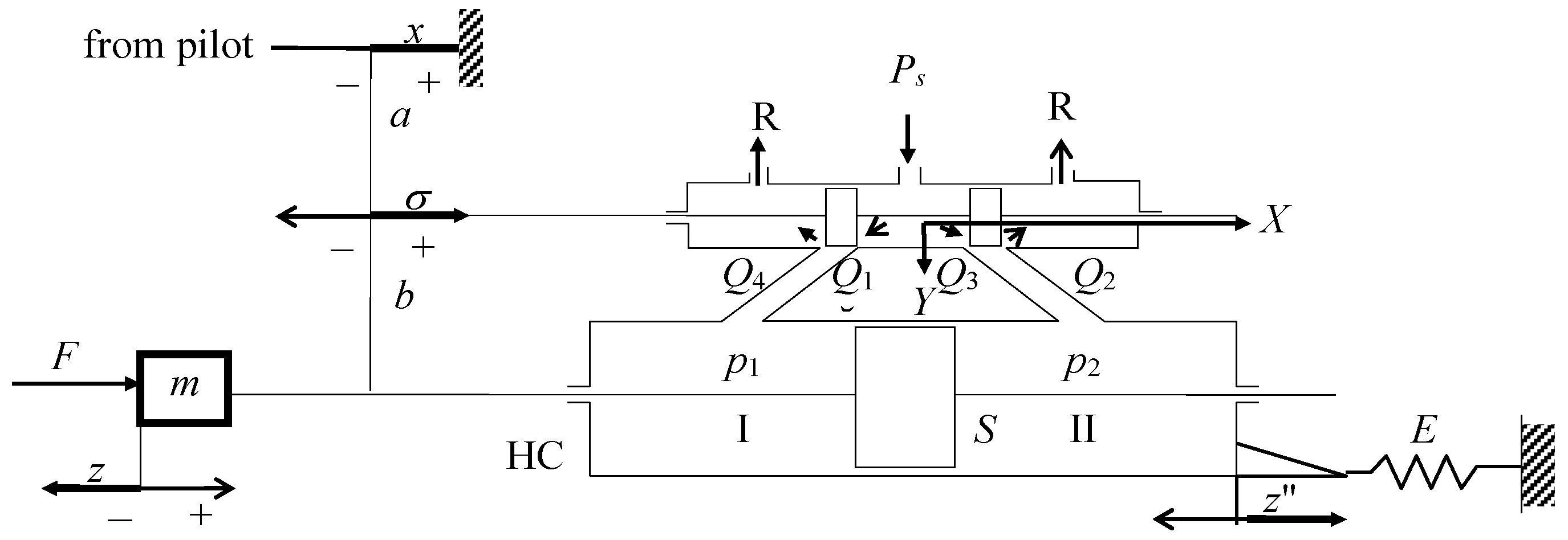
3. The Kinematics of the Rigid Feedback Linkage, the Impedance of the Mechano-Hydraulic Servomechanism and the Flutter Occurrence

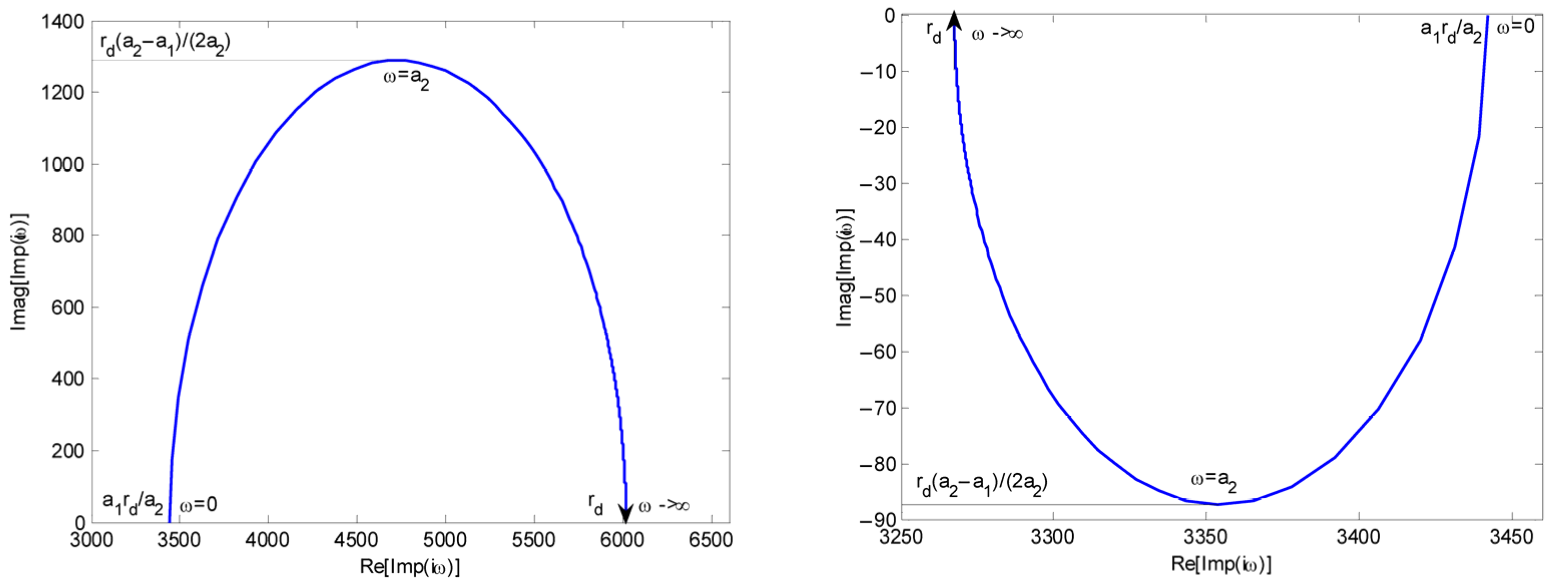
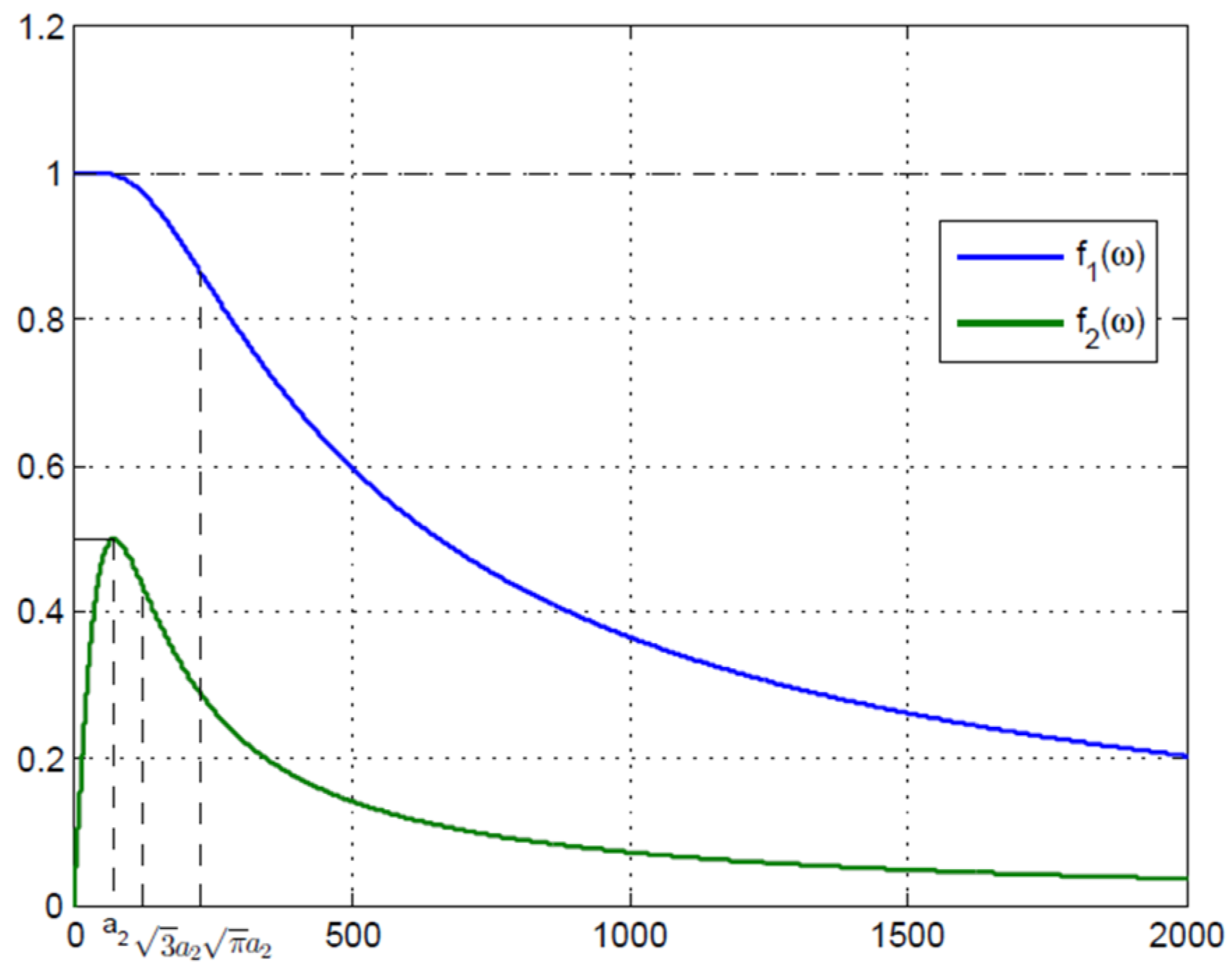
3.1. Impedance Mathematical Model

The servomechanism impedance, also known as dynamic stiffness, governs its response to output load variations. Formally, impedance is defined as the ratio, in a dynamic regime, between the output exerted force F and the displacement z induced by this force, under the assumption of a blocked input (x = 0), as shown in Figure 5.
Impedance is a complex variable function, and its calculation is derived from the simplified mathematical model given in Figure 5. The feedback linkage equation, generally taken as an algebraic linear equation connecting the input variable x , the output variable z , the displacement of mounting structure z and the control signal σ (also called “error”), will be herein given in the specific form [30]
σ = λ 1 x + λ 2 z λ 3 z , λ 1 : = b / a + b , λ 2 : = a / a + b , λ 3 : = 2 λ 2
In the case of Figure 1 bottom-left and Figure 5 the kinematic coefficients are λ 1 : = a / b , λ 2 : = a + b / a . The system of equations for deriving the impedance function is simple to write
S z ˙ z ˙ + k c p ˙ = k Q σ k Q p Δ p , σ = λ 2 z λ 3 z , F = S Δ p = E z , Δ p : = p 1 p 2
Some notations can be deduced from the figure; k Q * ,   k Q p * are, respectively, the flow gain and flow-pressure gain obtained by linearizing the flow-pressure characteristic of the distributor (5), and λ 2 ,   λ 3 are kinematic coefficients involving the values a, b. E is the mounting structure stiffness. Noting with F (s) and z (s) the Laplace transforms of the variables F (t) and z (t), the impedance function is expressed as (s = iω)
Imp i ω : = F s / z s = r d s + a 1 / s + a 2 a 1 = λ 2 k Q / S , a 2 = r d λ 3 k Q / E S + k Q p / S 2 , 1 / r d = 1 / E + k c / S 2
The impedance function characterizes the servomechanism’s ability to either absorb or amplify flutter oscillations in primary flight controls which are aerodynamically triggered. The theoretical and experimental analysis of this phenomenon has been a mandatory requirement in aviation regulations since the 1980s.
Graphically, the expression (43) represents a curve in the (Re(Imp(ω), Im(Imp(ω)) complex plane (Figure 6). More specifically, its location is determined by the order relation between the parameters a1 and a2 in the impedance function:
If a1 < a2, the curve is positioned in quadrant I, corresponding to the favorable case where the actuators absorb flutter oscillations, indicating the presence of effective positive damping within the system; this behavior creates a pseudo-active control.
If a1 > a2, the curve is positioned in quadrant IV representing the unfavorable case, where the actuator amplifies flutter oscillations, resulting in negative damping within the system.
In this framework, the real part of the complex impedance function serves as a measure of system rigidity, while the imaginary part quantifies system damping (or lack of damping). Dimensionally, both components are expressed in terms of rigidity. These properties were documented in Av. Regulation P. 970, which was introduced in the early 1980s. However, a comprehensive physical and mathematical proof of these principles is not readily available in the specialized literature.

3.2. Main Result

In the following, the energy foundation of the anti-flutter stability relationship a1 < a2 is demonstrated. This relationship can be interpreted as ensuring the flutter’s pseudo-active control by the hydraulic servomechanism through constructive and functional design conditions.
Proposition 1.
A sufficient condition for the anti-flutter stability of the (mechanical) hydraulic servomechanism is a1 < a2.
Proof. 
The energy balance method is applied. Let F represent the effort required to achieve the output displacement z = z 0 sin ω   t while the servomechanism is powered and the input remains blocked (Figure 5). Then, Φ = −F denotes the response effort of the servomechanism, which is exerted through energy received from external sources (hydraulic energy). This effort satisfies the equation
Φ ˙ = a 2 Φ r d z 0 ω cos ω t + a 1 sin ω t = a 2 Φ + A 1 sin ω t + B 1 cos ω t .
The produced effort Φ can be considered as being dissipated by the forces of inertia, viscous and elastic friction, leading to the equation
Φ = m z ¨ + f z ˙ + k z = A 2 sin ω t + B 2 cos ω t , A 2 = z 0 k m ω 2 ,     B 2 = z 0 f ω
The solution to Equation (44), given the initial condition Φ(0) = 0, is expressed as
Φ ( t ) = 0 t e a 2 τ A 1 sin ω τ + B 1 cos ω τ d τ e a 2 t
The consumed energy W 2 is compared with the energy received W 1 over a given time period
W 1 =   0   2 π / ω   0   t e a 2 t A 1 sin ω t + B 1 cos ω t d t e a 2 t   ω   z 0 cos ω t   d t , W 2 =   0   2 π / ω A 2 sin ω t + B 2 cos ω t ω   z 0 cos ω t   d t
where the expressions were obtained from the general relation W = Φ d z / d t d t . After performing the calculations, it follows that the delivered energy W 1 = r d ω z 0 2 a 1 a 2 π a 2 ω 1 e 2 π a 2 / ω / a 2 2 + ω 2 / a 2 2 + ω 2 , while the received (consumed) energy is W 2 = π z 0 2 f ω . The energy stability condition in the presence of flutter, W2 > W1, reduces to
r d a 1 a 2 π a 2 ω 1 e 2 π a 2 / ω / a 2 2 + ω 2 / a 2 2 + ω 2 < π f .
The graphs of the functions f 1 ω = 1 e 2 π a 2 / ω ,   f 2 ω = a 2 ω / a 2 2 + ω 2 (Figure 7) illustrate that the product f 1 ω f 2 ω remains sub-unitary and positive, thereby validating an increase in the left side of inequality (46), leading to the stability covering condition
r d a 1 a 2 / a 2 2 + ω 2 < f
Thus, if a1 < a2, the servomechanism’s damping effect on flutter oscillations is guaranteed for any pulsation ω; the condition is expressed as
λ 2 k Q / S < k Q / E + k Q p / S S E / S 2 + k c E
This relationship (48) is highly significant, as it emphasizes the importance of the coefficient k Q p * and the aeroservoelastic coefficients λ2 and E in flutter analysis. A numerical evaluation, based on nominal parameters of the SMHR servomechanism in the aileron control chain of the IAR 99 [6,35,36] confirms that inequality (48) is satisfied. The calculation data were λ2 = 2/3, λ3 = 4/3, m = 0.033 daNs2/cm, E = 7000 daN/cm, kQ = 624 cm2/s, S = 10 cm2, kQp = 0.02 cm5/(sdaN), and kc = 30/12,868 cm5/daN. However, the inequality is not fulfilled when the servomechanism has λ 2 greater than 1 (Figure 1 bottom-left. A servomechanism with an unsuitable impedance function cannot induce a pseudo-active control of flutter. To obtain the graph in Figure 6 at right, the value kc = 210/12 868 cm5/daN was considered. The essential result of this section is put, for eloquence, in Table 3.

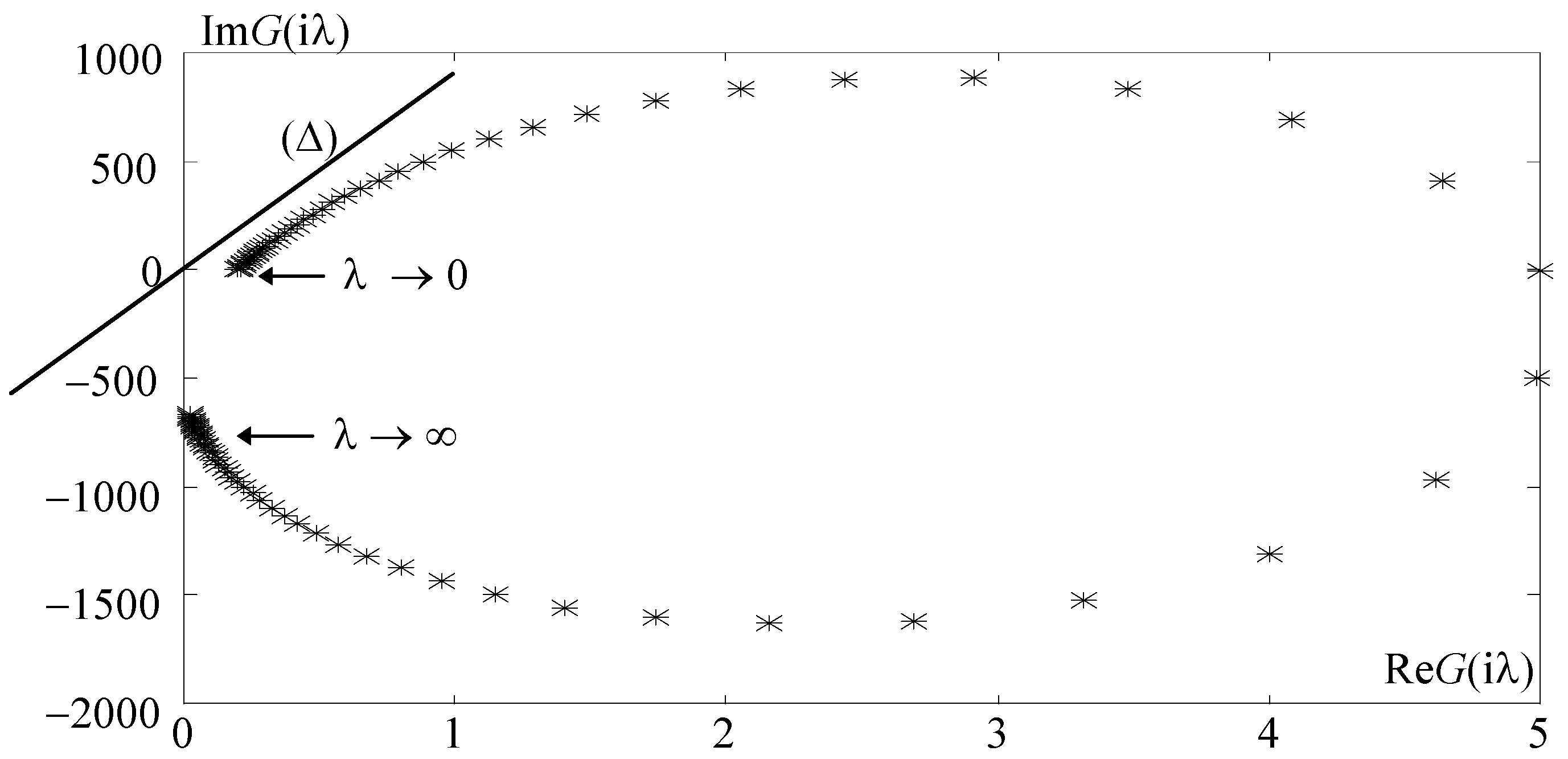
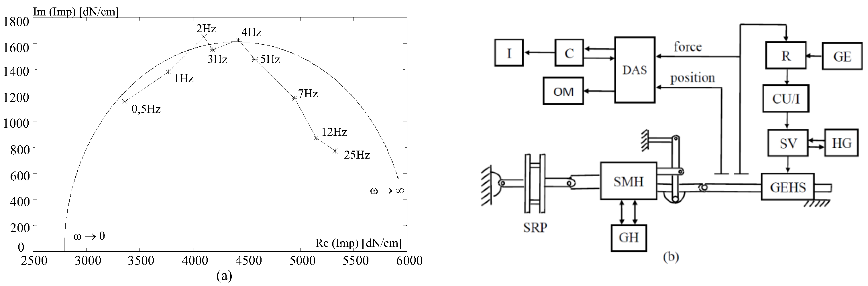
3.3. Impedance Function Measuring in Laboratory

Unlike a frequency response test, the experimental determination of servomechanism SMH impedance—illustrated in the block diagram of Figure 8b—requires the application of sinusoidal force signals at its output, using an electrohydraulic signal generator (GEHS), while its input remains blocked.
For a signal force of given amplitude and frequency, the ratio between the input force amplitude and the output displacement induced by this force is measured, along with the phase difference between the signals (all under stability conditions). The procedure is repeated while maintaining a chosen force amplitude across a range of frequencies extending from near-zero values to higher frequencies, ensuring the impedance measurement remains relevant (i.e., until normal frequency levels of aerodynamic disturbances—forces acting on control surfaces, or of mechanical vibrations of the servomechanism output adjacent structure, are exceeded).
For different values of force signal amplitude, distinct impedance curves are obtained. Fundamentally, the bench setup consists of the same devices and components as the frequency response bench, including mounting structure stiffness simulator (SRP), regulator (R), current strength-to-voltage converter, (CU/I), GEHS supply group comprising a servo-valve (SV) and a hydrostatic generator (GH), electrohydraulic signals generator (GE), data acquisition system (DAS), printer peripherals (I), memory oscilloscope (OM), and PC (C). An experimental impedance curve, determined for an output force amplitude of 125 daN, is reproduced from the INCAS Internal Reports (Figure 8a). This curve forms part of the approval programs for both the SMH servomechanism and the IAR 99 Hawk aircraft. The impedance test demonstrate compliance with regulations requirements and aligns with theoretical analysis, reinforcing its technical relevance.
In Figure 8a it is seen that there is naturally an acceptable difference between the theoretical and the experimental curve. The important thing is that the impedance characteristic is one with damping against flutter oscillations (the curve is located in quadrant one marking positive damping in the system from the SMH side)

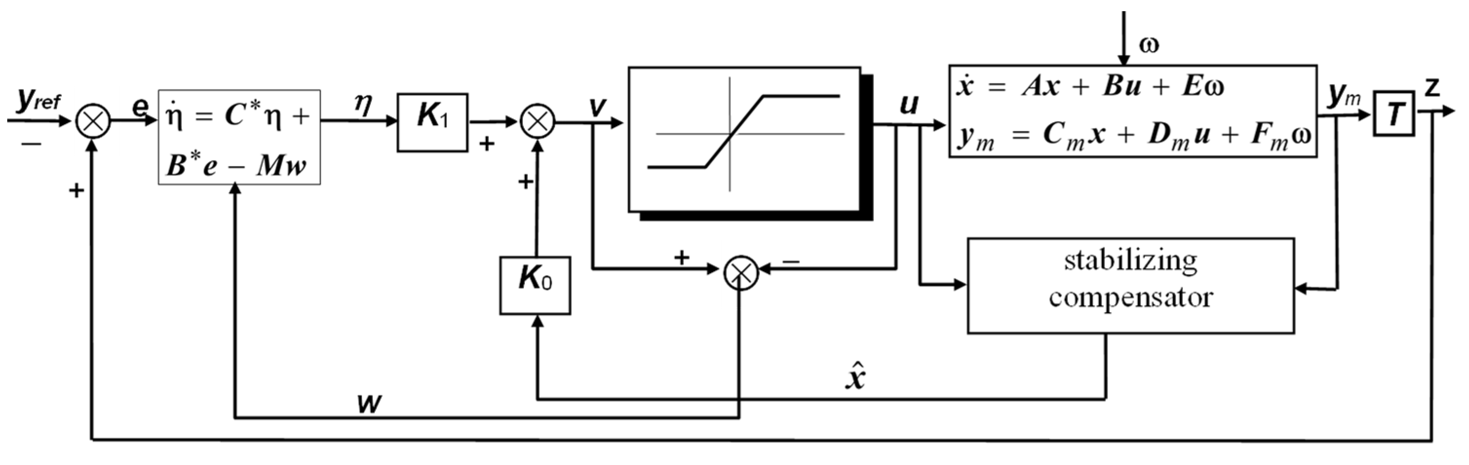
4. Robust Synthesis with Anti-Windup Compensation for Electrohydraulic Servomechanisms

4.1. Introduction

One of the main linear control design paradigms that emerged in the 1970s is robust control for a general servomechanism problem (RSP) [37,38]. This framework ensures that certain system outputs accurately follow reference commands, such as steps, ramps, sinusoids, or polynomial functions of time, under specified conditions, including disturbance rejection. The solution of RSP consists of two distinct components: a servo-compensator, in fact an internal model of the exogenous dynamics, and a stabilizing compensator. In the application of RSP to electrohydraulic servo-actuators, significant contributions were made in [4], specifically demonstrating that an optimal choice for the servo-compensator structure is an integrator for step inputs; so, achieving effective servo control necessitates integral action; however, integral action inherently induces harmful secondary saturating effects [38], particularly the reset windup phenomenon [39]. To mitigate this effect, an anti-reset windup (AW) strategy associated with the RSP solution was also proposed in [4]. These findings, the integral action as a general internal model and the AW strategy, compose an integrated methodology for addressing nonlinearities in an electrohydraulic servo system. This assertion is supported by the following: (1) the equations governing load movement in an electrohydraulic servo system exhibit strong nonlinearity [36] and can be accurately linearized [40] only in the presence of small inputs; (2) according to the sampled data paradigm, a system’s response to (small) step inputs is representative, considering the sampling procedure for general reference signals; (3) thus, only control saturation-type nonlinearity remains to be counteracted.

4.2. Robust Servomechanism Problem

Consider the plant to be controlled described by the following linear time-invariant model
x ˙ = A x + B u + E ω , z = C x + D u + F ω   y m = C m x + D m u + F m ω ,   e = z y r e f
where x R n is the state of the system, u R m is the control, z R   r is the regulated output, y m R r m is the measurable output, ω R Ω is the disturbance, y r e f R r is the reference input and e R r is the error in the system. The regulated output z is taken physically measurable, i.e., there exists T so that z = Tym. All matrices are of compatible dimensions throughout the formulation. The class of reference input and disturbance signals is described by the following two systems
w ˙ 1 = A 1 w 1 ,   ω = C 1 w 1 , w ˙ 2 = A 2 w 2 ,   σ = C 2 w 2 ,   y r e f = G σ
(w1 R n 1 , w2 R n 2 ), having the eigenvalues λi of A1 and A2 all with Re(λi) ≥ 0 and the pairs ( C i   ,   A i ) , i = 1, 2, observable. We will state the following problem:
Problem 2 (the Robust Control of a Servomechanism Problem (R.S.P.) [37,41,42]). 
Find a controller for system (49) such that when applied to this system, the following apply: (1) the resultant closed-loop system is asymptotically stable; (2) asymptotic tracking occurs, i.e.,  lim t   e ( t ) = 0 , (∀) x(0)∈Rn, for all initial conditions  ω ( 0 )  and yref(0); (3) condition (2) holds for any variations in the plant model (49) (including dynamic perturbations) that do not induce instability in the controlled system.
A fundamental theorem yields the solution of the RSP.
Theorem 3 ([42]). 
 A necessary and sufficient condition for the existence of a linear time-invariant controller for (49) such that e0 as t → ∞ for all measurable or unmeasurable disturbances described by linear time-invariant finite dimensional unstable autonomous systems, and for all specified reference inputs yref described by the same type of dynamic systems, while guaranteeing the stabilizabilty of the controlled system, is that the following conditions all hold: (1) (A, B) is stabilizable; (2) (Cm, A) is detectable; (3)  m r  ; (4) the transmission zeros of the quartet (C, A, B, D) do not coincide with the eigenvalues of the references and, respectively, disturbances system matrices; (5) z is physically measurable.
In Figure 9, the nonlinear saturation element and the compensation matrix M, which will be introduced in Section 4.4, must temporarily be disregarded: consequently, in the figure, let us consider u v . The controller structure is established by the following lemma.
Lemma 1 ([41,42], controller structure). 
Assume that conditions (1)–(5) of Theorem 3 are satisfied. Then, any controller that solves the R.S.P. for Equation (49) must have the structure u = K0 xc+ K1η, where xc is the output of the so-called stabilizing compensator and η is the output of the so-called servo-compensator.
The servo-compensator design is straightforward [42]. Let the minimal polynomial of A1, A2 be denoted as Λ1(s), Λ2(s), respectively, and let the least common multiple of Λ1(s), Λ2(s) be given by Λ(s). Let the zeros of Λ(s) (multiplicities included) be given by (λ1, λ2, …,λq). Let the coefficients δi, i = 1, …, q, be defined by the coefficients of the polynomial Π i = 1 q ( s λ i ) ; finally, let C* be the associated q × q companion matrix. Thus, in the simplified scalar case, the servo-compensator takes the form (Figure 9):
η ˙ = C * η + B * e ,   B * T = 0 0 0 b R q C * = 0 1 0 . . 0 0 0 1 . . 0 . . . . . . 0 0 0 0 0 1 δ 1 δ 2 δ 3 . . δ q
η =1, …, ηq), B * is a real matrix of rank 1 (with the property that (C*,B*) is controllable). As for the stabilizing compensator, this is not a unique device and may be constructed by using a number of different techniques, particularly that of an observer-type device.

4.3. Contributions to Servo-Compensator and Stabilizing Compensator Choices in the Case of Electrohydraulic Servo

Taking into account (49), we write the system
x ˙ = A x + B u + E ω , z = C x : = y o ,   e = z y r e f A = 0 1 0 k / m f / m S / m 0 S / k c k Q p / k c ,   B = [ 0 0 k u / k c ] T C = k p 0 0 ,   E =     [   0     1   0   ] T
where [.]T denotes the transpose of [.]; x = x 1 x 2 x 3 T is the state variables vector in which x1—the rod displacement, x2—the rod velocity, x3—the pressure difference between the cylinder chambers, caused by external load (inertial, elastic and perturbation forces); u—the control, measured in V; the input current to servo-valve, measured in mA, is i ,   i =   k V m A u , with kVmA measured in mA/V); y0—the measured output, here identical to regulated output z: = x1; yref—the reference input (command), measured in V; e—the error; ω —step and/or sinusoid-type state disturbance; m—the equivalent inertia load of primary control surface reduced at the rod; k—the equivalent spring stiffness; f—the equivalent damper coefficient; S—the piston active area; k Q p —the derivative of the flow characteristic with respect to the differential pressure between the cylinder chambers, see, [40,43]; k c = V / 2 B u , where V is the cylinder semi-volume and Bu is the bulk modulus of the hydraulic fluid used; k s v , measured in cm3/(smA), is the derivative of the flow characteristic with respect to the input (control) electrical current of the servo-valve and ku = ksvkVmA; kp, measured in V/cm, is the gain of the position transducer.
Servo-compensator device. Concerning the structure of the servo-compensator, one states the following conjecture.
Conjecture 1.
In a large number of cases, the servo-compensator designed for step inputs  η ˙ = e  represents a good choice.
The procedure outlined in [44] is considered in building the polynomial Λ ( s ) , where the bandwidth [ ω b ,   ω b ] is divided into 2Nω − 1 segments each of width  ω 0 , and Nω = ω b / ω 0 + 1/2. The spectrum is approximated by impulses in ± k ω 0 , k = 0, …, Nω − 1. Consequently, the signals ω and yref will be approximated by linear combinations of sinusoids, including step signals:
  Λ ( s ) = s [ ( s 2 + ω 0 2 ] × [ s 2 + ( 2 ω 0 ) 2 ]     [ s 2 + ( ( N ω 1 ) ω 0 ) 2 ]
The chosen formulation allows a simple numerical assessment of the coefficients depending only on p = Nω 1 and ω b = ω 0 ( N ω 1 / 2 ) in the equation
1 δ m a x η ˙ 2 p + 1 = δ 2 δ m a x η 2     δ 2 p δ m a x η 2 p + b δ m a x e
where δmax = max(δ2, …, δ2p), η = (η12, …,η2p+1)T and η1: = η. To clarify the proposed conjecture, the understood inference follows by analyzing Table 4, where 0 denotes a negligible number. (Certainly, b can be selected such that b = δ m a x ; for the sake of simplicity, ωb was chosen natural, and the resulting ω0 is rational).
Stabilizing compensator device. Consider xcx, i.e., the stabilizing compensator is simply a direct measurement of the state; so, the controller is feedback for the augmented state system comprising the plant (52) and the servo-compensator (51): u = K 0 x + K 1 η . So, a standard optimal linear quadratic stabilization problem can be defined for the extended system
x ˙ η ˙ = A O B * C C * x η + B O u ,   z = O D ˜ x η , D ˜ = 1     ?     0 R q
with the usual performance index min u J , J J ( u ) =   0   ( z 2 Q J + u 2 R J ) d t . The solution K 0 K 1 is obtained from the well-known associated Riccati equation
  X ˜ A O B * C C * + A O B * C C * T X ˜ X ˜ B O R J 1 B O T X ˜ + O T D ˜ T Q J [ O   D ˜ ] = O ,   K 0 K 1 = R J 1 B O T X ˜

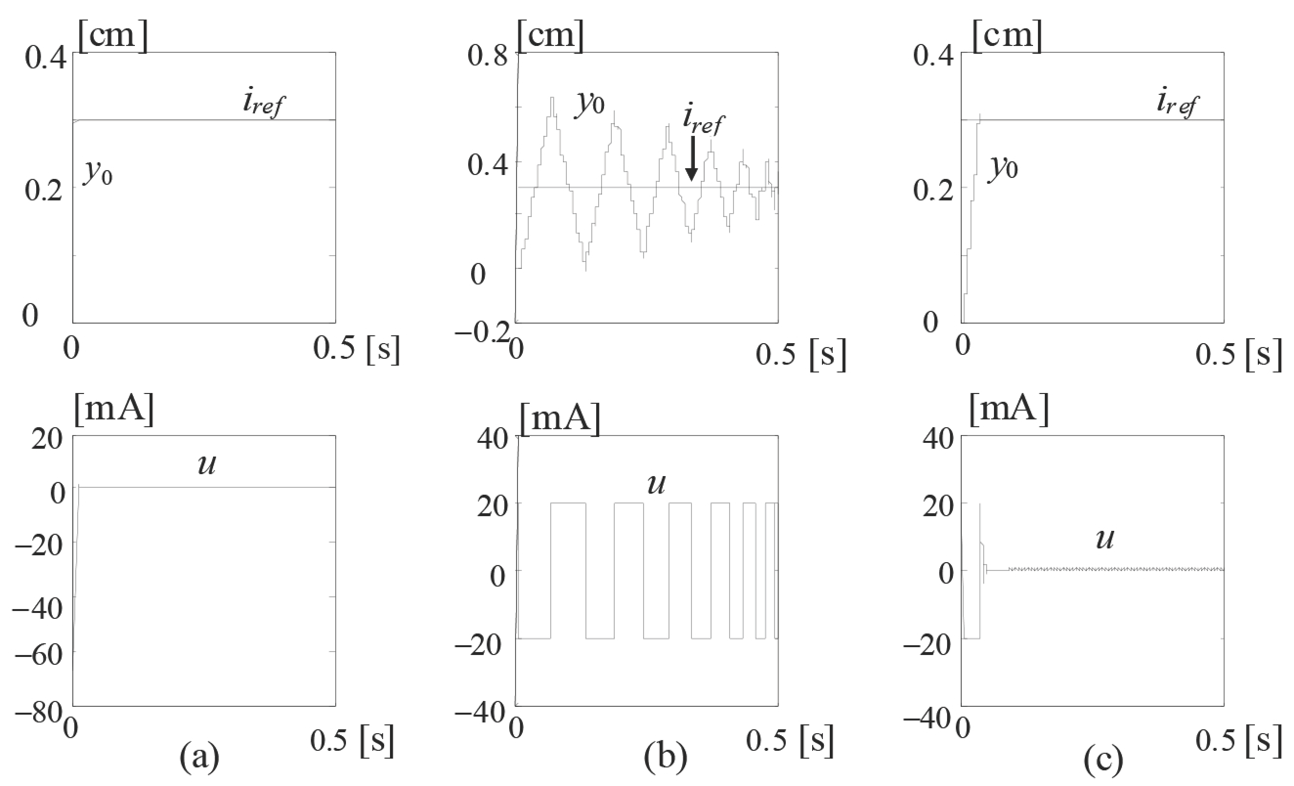
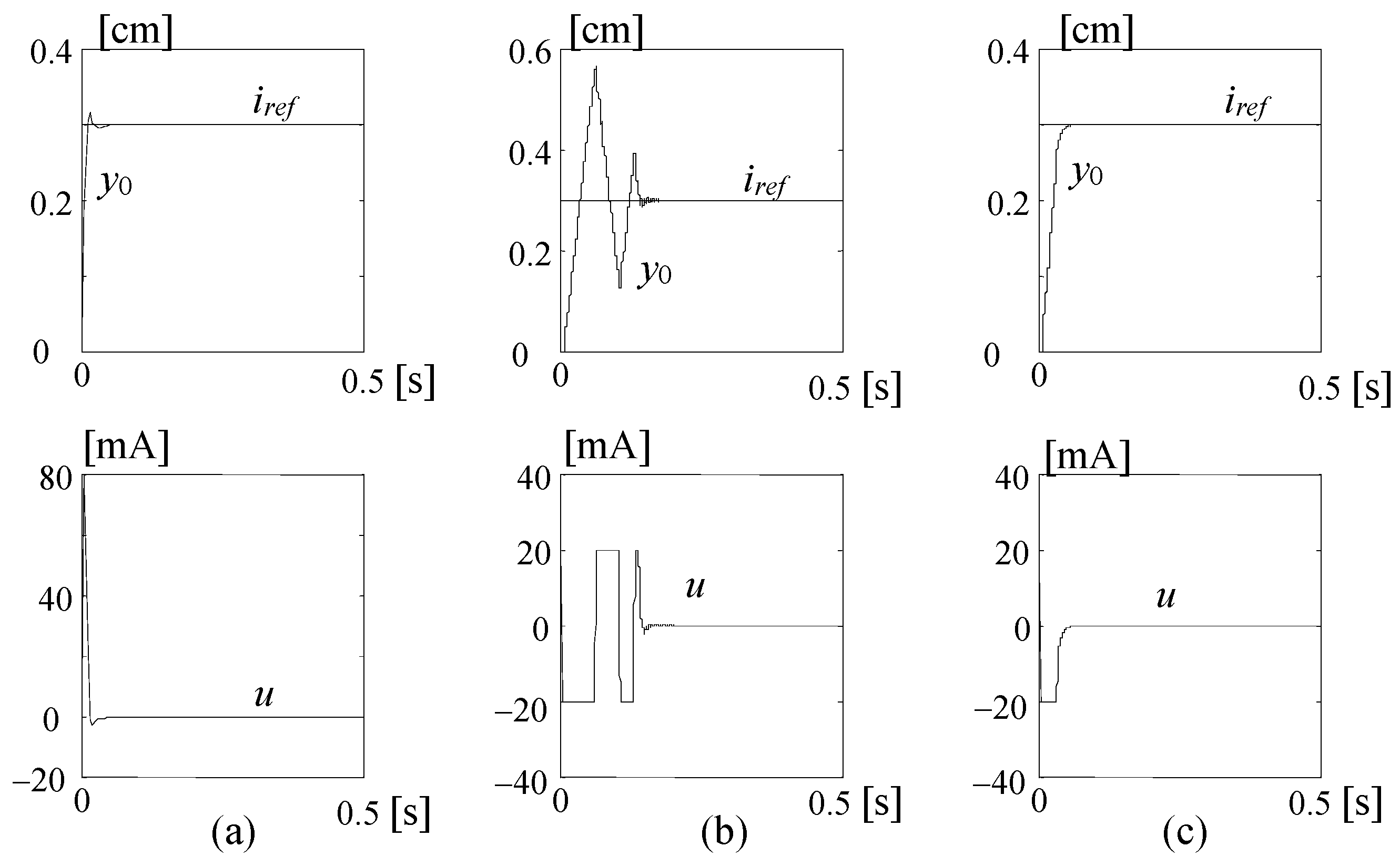
4.4. Anti-Windup Compensation of the Saturating Electrohydraulic Servo

When actuator saturation is ignored, the phenomenon known as reset windup can produce the worst undesirable transients. Indeed, in many aerospace engineering applications, actuator saturation is often the principal impediment in achieving significant closed loop performance. It is worth noting that integral action, discussed earlier, can rapidly improve the saturation level [38]. Thus, various anti-reset-windup (AW) strategies have been presented lately in the literature to address actuator limitations. In the following, an AW procedure proposed by the authors, see [4], is briefly presented, along with the proof of a proposition that defines the AW compensation matrix. Assuming a new conjecture, the derivation of the compensation matrix M (Figure 9) is a result of the constraint to make the state of the saturated system arbitrarily close to the state of the unsaturated system whenever the actuator reaches saturation. So, the two systems
x ˙ = A x + B u ,   y = C x ,   u = sat ( v ) ,     η ˙ = C * η + B * e M ( v u ) , v = K 0 x + K 1 η ,     e = y r , r : = y r e f
operating in a closed loop, are analyzed, in the absence and the presence of saturating actuators (the function sat(.) is represented in Figure 9), respectively, in the linear case u = v and the nonlinear saturating case u = sat(v). By concatenating, the systems (13) will be obtained, at equilibrium stationary points, in a linear case or nonlinear case
x η s t l = A + B K 0 B K 1 B * C C * 1 O B * r ,   x i η i s t n = A O B * C M K 0 C * M K 1 1 B s a t i ( v ) M s a t i ( v ) + B * r  
The index i denotes whether v falls within the linear region, exceeds the upper limit, or drops below the lower limit of the saturation range. A question thus arises: what matrix M ensures
min M J , J = i = 1 2 ( x s t l x s t n   , i ) T ( x s t l x s t n   , i ) + i = 1 2 ( η s t l η s t n   ,     i ) T ( η s t l η s t n   , i )
The solution of problem is given by the following
Proposition 2.
The AW compensation matrix  M = B * C A 1 B K 0 A 1 B + I 1  ensures a minimum of J (if A and  I + K 0 A 1 B  are non-singular).
Proof. 
By applying the inversion lemma [45]
P Q R S 1 = X X Q S 1 S 1 R X W ,     X : = P Q S 1 R 1 , W : = S 1 + S 1 R X Q S 1
to Equation (58), one obtains
A   O B * C M K 0   C * M K 1 1 = A 1 O C * M K 1 1 B * C M K 0 A 1 C * M K 1 1
Noting that the matrix M appears only in the second row of the previous equality and only the entry (2, 2)
W = C * 1 + C * 1 B * C A + B K 0 B K 1 C * 1 B * C 1 B K 1 C * 1
of the first inverted matrix in (14) counts, the difference between the servo-compensator’s stationary points is
η s t l η s t n , i = W B * r C * M K 1 B * C M K 0 A 1 B s a t i v C * M K 1 1 B * r M s a t i v = = W C * M K 1 1 B * r C M K 1 1 B * C M K 0 A 1 B M s a t i v
If the matrix M is given by B * C A 1 B K 0 A 1 B + I 1 , the factor of the saturation function sat i v   is eliminated. A remarkable observation is that the same value of M also cancels the other term, leading to the verification of
          C * 1 + C * 1 B * C A + B K 0 B K 1 C * 1 B * C 1 B K 1 C * 1 C * M K 1 = I
or, with some calculus (by reducing the terms and simplifying with C*−1 O , K 1 O )
  B * C A + B K 0 B K 1 C * 1 B * C 1 B = M + B * C A + B K 0 B K 1 C * 1 B * C 1 B K 1 C * 1 M
Additionally, verifying
B * C A + B K 0 B K 1 C * 1 B * C 1 B B K 1 C * 1 M M 1 = I
assuming M is non-singular, leads to the final proof requirement
B M 1 K 1 C * 1 = A + B K 0 B K 1 C * 1 B * C π C 1 B * 1
which is easily verified by substituting M and expanding the parentheses. □

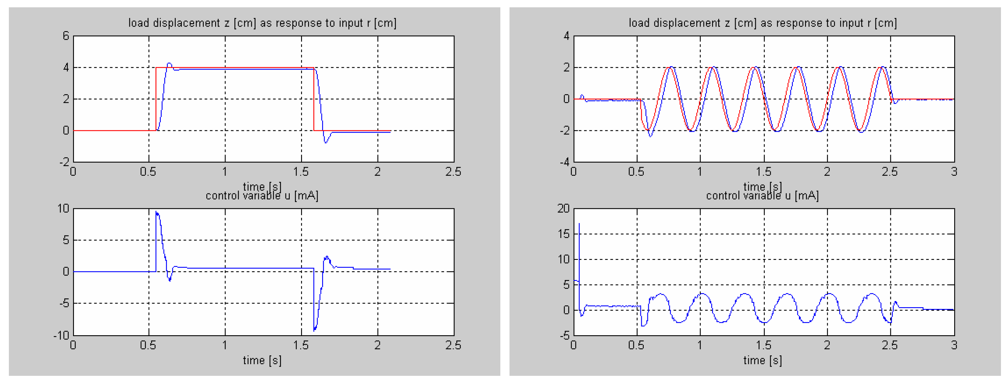
4.5. Numerical Application

The verification of all conditions in Theorem 3 as applied to system (52), was successfully completed using the ctrb, obsvf, tzero, ctrb from MATLAB R2016a. To illustrate the dynamic performances achievable through robust synthesis with anti-saturation compensation, the mathematical model of the SMH servomechanism, integrated into the control chain of the IAR 99 aircraft aileron, was selected as a benchmark. Given that this servomechanism operates in a mechano-hydraulic framework, its “passive” electrohydraulic equivalent (lacking a compensator in its internal loop) was considered as an exercise with the mathematical model described by the equation
x ˙ = A 1 x + B i r e f + E ω
where A 1 A , excepting A ( 3 ,   1 ) = k u k p / k c . kp is a position gain measured in V/m and ku = ksvkVmA is measured in m3/(Vs); the displacement of the servomechanism’s rod z is regulated output, and the associated reference, in V, is actually a commanded output converted into cm (1 V corresponds to 0.3 cm) (Figure 10).
A relatively good tracking of reference signals is possible with the “passive’’ electrohydraulic servomechanism integrated into the aileron control chain of a Romanian jet fighter (m = 30 kg) but only in the absence of ω-perturbations; otherwise, the reference tracking is entirely distorted [4]. In contrast, when employing an internal model (54) of order n = 0, 1 or 2, the system demonstrates good robustness in reference tracking even for frequencies not explicitly included in the internal model. In fact, the best tracking performance is achieved when using a pure integrator servo-compensator.
Figure 10 and Figure 11 illustrate the positive effect introduced by considering the antiwindup matrix M but also the importance of appropriate weights QJ and RJ. Thus, Figure 10 and Figure 11 shows both the harmful effects of saturation and the effectiveness of the proposed AW compensation in the real nonlinear case. The simulation was conducted using the weights QJ = 1013 and RJ = 1 with the feedback gain [K0 K1] = K 0 K 1 = 486.12 0.11 0.13 3163 . The result is remarkable, as it (a) validates the choice K 0 x + K 1 η of the servo compensator not to be invalidated as unrealistic and (b) highlights the feasibility of relying solely on x position, which simplifies implementation by eliminating the need for velocity and pressure transducers. In Figure 11, where weights QJ = 109 and RJ = 1 were used, the results are much better and emphasize the importance of the careful tuning of weights parameters to mitigate control chattering, which directly impacts system performances. The step reference input was iref = 1 V, corresponding to a controlled output displacement of 0.3 cm. While the feedback vector in a robust synthesis depends on a mathematical model of the servomechanism, this methodological limitation can be avoided using neuro-fuzzy synthesis, as will be discussed in the next section.
For the simulations, a pure integrator type servo-compensator was employed with system parameters as follows: k = 105 N/m, f = 103 Ns/m, S 10 3 m2, kc = 0.25 × 10 13 m5/N, kp = 103/3 V/m, kQp = 0.523 × 10 12 m5/(Ns), ku = 10 5 m3/(Vs), m = 30 kg. The parameter ku represents the product kSVkVmA between the flow/current gain of the servo-valve and the current/voltage gain kVmA; consequently, the considered saturation level was ±10 V in the control u, or ±20 mA in the current to servo-valve, since kVmA was considered 2 mA/V. The frequency selection for the internal model in the domain [0,1] Hz is νi = i/(Nω − 1), i = 1 ÷ Nω − 1.
Final note of Section. To summarize, the theoretical framework and key findings of Section 4 are: Problem 2, Theorem 3, Lemma 1, Conjecture 1, stabilizing compensator structure, Proposition 2.

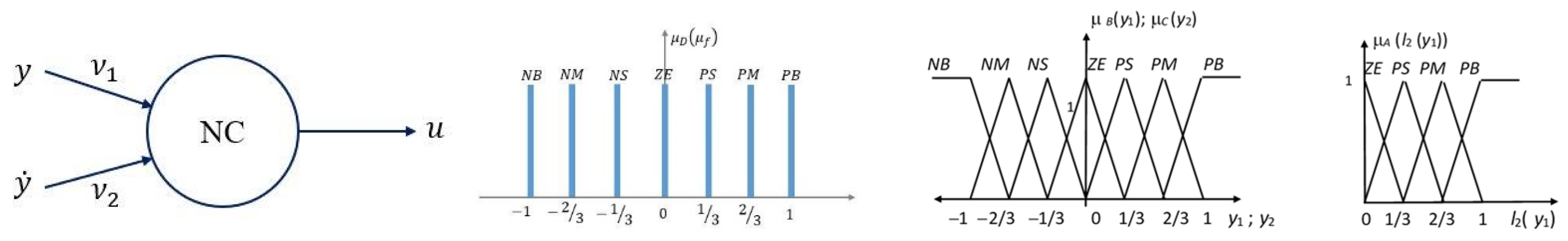
5. Neuro-Fuzzy Synthesis of Electrohydraulic Servo for Motion Control—Experimental Validation

5.1. Introduction

This section addresses the problem of laboratory test validation of an electrohydraulic motion control system (EHMCS) based on neuro-fuzzy synthesis. Previously, the fuzzy supervised neurocontrol (FSNC) of a similar electrohydraulic servomechanism was explored in a theoretical framework, with validation relying on numerical simulations, as presented in [11,46]. A LabView implementation of the algorithm was conducted, and simulation results demonstrated the effectiveness of the neuro-fuzzy control compared to classical approaches such as PID, LQG, etc. The control algorithm, referred to as the Fuzzy Supervised Neurocontrol (FSNC), for an Electro-Hydraulic Motion Control System (EHMCS) is developed and experimentally tested. The EHMCS (Figure 12) consists of several components: a double effect hydraulic cylinder with the piston area and half of piston stroke and an ORSTA TGL33649 electrohydraulic (servo)valve. The valve is a direct valve, in which a linear motor drives the spool directly according to the input current. The valve has a nominal flow of 40 × 10−3 m3/60 s at the nominal pressure drop of 70 bar. A PC controls the system through a DAQ PCI 6040E National Instruments. An inductive position transducer manufactured by Penny & Gilles and two Hottinger Baldwin Messtechnik (HBM) pressure transducers provide the measurement input for DAQ. The inertial load is simulated by an inertial load simulator and the hydraulic power is supplied by a hydrostatic generator.

5.2. FSNC Description

The EHMCS operates fundamentally as a tracking system where the objective of control synthesis is to ensure precise piston position based on the specified desired position references introduced as electrical signals from the PC. In classical control approaches, solving this problem requires two primary steps: developing a mathematical model of the system and applying a control synthesis method based on this model. Nevertheless, the classical methodology is model-dependent, and no model is perfectly accurate. The traditional control methods often struggle with the mathematical complexity associated with real-world objects. This complexity is evident in detailed mathematical models presented in works such as, [29,47]. For instance, a non-exhaustive mathematical model of the system described above is formulated as follows
m x ¨ + f x ˙ + k x + F + F f = S p 1 p 2 ,     x v = k x v u u p ˙ 1 = B C + S x c w x v sgn p s 1 + sgn x v 2 p 1 p s ( 1 + sgn x v ) 2 p 1 / ρ S x ˙ p ˙ 2 = B C S x c w x v sgn p s 1 sgn x v 2 p 2 p s ( 1 sgn x v ) 2 p 2 / ρ + S x ˙ F f = σ 0 x f + s 1 x ˙ f + f v x ˙ , x ˙ f = x ˙ x ˙ x f / g x ˙ , g x ˙ : = F c + F s F c e x ˙ / v s
The nomenclature in (62) is given in the cited author’s references and will not be repeated here. k p is the position transducer coefficient [V/m]. The mathematical models under consideration serve primarily to identify, through numerical simulation, the parameters defining the artificial intelligence system. In an online process, the mathematical model is naturally substituted by the physical system.
Problem 3 (control FSNC).
Given the mathematical formulation of the EHMCS, classical solutions of the control problem “find control variable u such that tracking error  ε t : = r t k p x t 0  as  t  for specified reference signals  r t ” face obvious challenges due to system complexity.
The proposed FSNC structure is briefly described below. The algorithm is composed of a neurocontrol and a fuzzy logic control supervising neurocontrol. The neurocontrol module is designed using a single-layered perceptron architecture. Within this elementary network, two weighting parameters ν 1 , ν 2 and a linear combiner generate the neurocontrol function (Figure 13)
u n = ν 1 y 1 + ν 2 y 2 = : ν 1 ( r k p z ) + ν 2 p 1 p 2
where r t —reference input (command) ([V]). From the EHMCS behavior perspective, the input is u and the output is y = y 1 , y 2 . From the neurocontrol training perspective, the system performance is assessed by the cost function, which balances tracking error, the second input component y 2 , and the control u
J = 1 2 n i = 1 n q 1 y 1 2 i + y 2 2 i + q 2 u n 2 i : = 1 2 n i = 1 n J i
The weighting vector ν = [ ν 1   ν 2 ] T is updated online using the gradient descent learning method [48] to minimize the cost function J. Accordingly, the update is defined by the expression
ν ( n + 1 ) = ν ( n ) + Δ ν ( n ) Δ ν ( n ) :   = d i a g ( δ 1 , δ 2 ) J / ν ( n ) = d i a g ( δ 1 , δ 2 ) i = n N n J ( i ) y ( i ) y ( i ) u ( i ) + J ( i ) u ( i ) u ( i ) ν ( i )
where the matrix d i a g ( δ 1 , δ 2 ) introduces the learning scale vector, Δ ν ( n ) is the weight vector update and N marks a back memory (of N time steps). The derivatives in (66) require only input–output information from the system. y ( i ) / u ( i ) is online approximated by the relationship ( y ( i ) y ( i 1 ) ) / ( u ( i ) u ( i 1 ) ) . Simulation results demonstrate highly satisfactory performance using this simple single-layer perceptron. For compliance, the derivatives from relationship (65) are written explicitly as follows:
Δ ν n : = d i a g δ 1 , δ 2 M i ; n , N M i ; n , N = i = n N n J i y 1 i y 1 ( i ) y 1 ( i 1 ) u ( i ) u ( i 1 ) + J i y 2 i y 2 ( i ) y 2 ( i 1 ) u ( i ) u ( i 1 ) + J i u i u i ν 1 i u i ν 2 i M i ; n , N = i = n N n 2 q 1 y 1 ( i ) y 1 ( i ) y 1 ( i 1 ) u ( i ) u ( i 1 ) + 2 q 2 y 2 ( i ) y 2 ( i ) y 2 ( i 1 ) u ( i ) u ( i 1 ) + 2 q 2 u ( i ) y 1 ( i ) y 2 ( i )
Actuator saturation is a major challenge in many applications, particularly in aerospace engineering, where it significantly limits closed-loop performance [4,49]. In a neural network-based learning process, the risk of control saturation is a real concern. If not properly addressed, it can lead to undesirable effects such as control chattering and degraded system performance. To mitigate this risk, FSNC is considered within the framework of an AW strategy. The commonly used Mamdani fuzzy logic control supposes three main components: the fuzzyfier, the fuzzy reasoning, and the defuzzyfier [50]. Herein, the proposed fuzzyfier component converts the crisp input signals
l 2 ( y 1 k ) : = j = k 2 k y 1 j 2 ,   y 1 k ,   y 2 k ,   k = 1 ,   2 ,
into their relevant fuzzy variables (or, equivalently, membership functions) using a set of linguistic terms: zero (ZE), positive or negative small (PS, NS), positive or negative medium (PM, NM), positive or negative big (PB, NB); thus, fuzzy sets and their pertinent membership functions are produced (for the sake of simplicity, triangular and singleton type membership functions are chosen; see Figure 13). The l2 norm is utilized to compute, over a sliding window of k samples, the maximum variation in tracking error. Introducing this crisp signal in the fuzzyfier will result in a reduction in fuzzy control switches due to the effects of spurious noise signals [51].
The fuzzy reasoning construction is based on the principle of a (direct) proportion between the error signal y1 and the required fuzzy control uf. Herein, the fuzzy reasoning engine is designed to include n = 4 × 7 × 7 IF …, THEN … rules, which correspond to the elements of the Cartesian product A × B × C, A: = {ZE; PS; PM; PB}, B = C: = {NB; NM; NS; ZE; PS; PM; PB}. These sets are associated with the sets of linguistic terms chosen to define the membership functions for the fuzzy variables l 2 y 1 , y1 and, respectively, y 2 . Consequently, the succession of the n rules follows the structure:
(1) IF l2 (y1) is ZE and y2 is PB and y1 is PB, THEN uf is PB; (2) IF l2 (y1) is ZE and y2 is PB and y1 is PM, THEN uf is PM; (7) IF l2 (y1) is ZE and y2 is PB and y1 is NB, THEN uf is NB; (8) IF l2 (y1) is ZE and y2 is PM and y1 is PB, THEN uf is PB; (196) IF l2 (y1) is PB and y2 is NB and y1 is NB, THEN uf is NB
Let τ be the discrete sampling time. Consider the three scaled crisp input variables l2 (y1k), y1k and y2k, at each time step t k = k τ (k = 1, 2, …). Taking into account the two ordinates corresponding to each of the three crisp variables in, Figure 13 a number of M  23 combinations of three ordinates must be investigated. Based on these combinations, a number of M IF…, THEN… rules will operate in the form
IF   y 1 k   is   B i   and   y 2 k   is   C i   and   l 2 y 1 k   is   A i ,   THEN   u f k   is   D i ,   i = 1,2 , , M
(Ai,B, Ci, Di are linguistic terms belonging to the sets A, B, C, D and D = B = C; see, Figure 13). The defuzzyfier concerns the transforming of these rules into a mathematical expression that defines the output control variable uf. In terms of fuzzy logic, each rule of (68) defines a fuzzy set Ai × Bi × Ci × Di in the input–output Cartesian product space R + × R3, where the membership function is formulated as
μ u i = min μ B i y 1 k , μ C i y 2 k , μ A i l 2 y 2 k , μ D i u , i = 1 , , M , k = 1,2 , ,
For simplicity, the singleton-type membership function μD(u) has been chosen for the control variable. In this case, μ D i ( u ) is replaced by u i 0 , which is the singleton abscissa. Therefore, using (1) a singleton fuzzyfier for uf, (2) a center-average type defuzzyfier, and (3) the min inference method, the M IF…, THEN… rules can be transformed, at each time step kτ, into a crisp control formula u f [52]:
u f = i = 1 M μ u i u i 0 / i = 1 M μ u i
The FSNC operates as a fuzzy logic controller whenever the neurocontrol saturates, or when the l2-norm of the tracking error y1 increases. FSNC switches on neurocontrol whenever u n does not saturate ( u n u n , m a x ) and the scaled l 2 ( y 1 ) is less than l2,min, l 2 ( y 1 ) <  l2,min. During fuzzy control operation, the fuzzy neurocontrol un is continuously updated by considering the real acting fuzzy control uf. Since it is preferable for the system to be governed by (quasi)optimal neurocontrol, fuzzy logic switches neurocontrol on whenever u n is not saturated and whenever the scaled norm l2 (y1) is below a predefined threshold l2,min. To ensure a smooth transition at switching time t s , when control shifts from fuzzy logic control to neurocontrol, the weighting vector ν r must be adjusted by applying a scale factor u f u n as defined in [11]
ν 1 r = u f ν 2 y 2 u f u n y 1 ,   ν 2 r = ν 2 u f u n .
After several inherent explorations conducted on the mathematical model (63) the parameters of the neuro-fuzzy control law were fixed: initial weighting vector (see (64) ν 0 = ν 10 , ν 20 : = 0.01 , 0.01 , the weights of cost function (65) q 1 , 1 , q 2 : = 300 , 1 , 0.1 , and the learning rates (see (4)) δ 1 , δ 2 : = 0.05 ,   0.0004 . For scaling operation of the quantities, the following value was used for the control variable: u m a x = 10   V . For y 1   m a x ,   y 2   m a x , the maximum values were determined by the size of the references and, respectively, by the maximum supply pressure of the EHMCS.

5.3. Numerical Application

Despite the physical model’s complexity, the laboratory tests performed on the EHMCS with the FSNC algorithm attested strong tracking performance, under the step and sinusoidal reference signals r, as shown in Figure 14. These promising results highlight the effectiveness of the approach and provide strong motivation for further advancements in intelligent control strategies [15,16].
The proposed FSNC offers significant advantages over the system presented in [4], since in that approach, the synthesis is dependent on a linear model of the controlled system. This new approach to control synthesis accounts for the saturation nonlinearity and provides in addition anti-chattering and robustness properties to the controlling system. Indeed, the obtained control solution is highly promising to be robust since it does not demand a model of the system.
Here is the path for the synthesis of the FSNC.
1. If a mathematical model of the driven object is available (in this case, the servomechanism equations), the FSNC parameters will be tuned to this model, thus saving time when moving on to the online process.
2. If a mathematical model is not available, go directly to the implementation of the FSNC online.
Go to the synthesis of the neurocontrol with fuzzy supervisory control.
1. Synthesis of the neurocontrol: the relations (64)–(67) are calculated; the simplest variant was chosen, elementary perceptron NC, as shown in Figure 13.
2. Synthesis of the Mamdani-type fuzzy control with the following steps: the fuzzyfier, the fuzzy reasoning, and the defuzzyfier.
3. The reciprocal switching logic between neurocontrol (64) and fuzzy control (71) is specified.

6. A Brief Overview of Some Recent Results in Hydraulic Servomechanisms

This section provides a concise overview of theoretical results concerning mathematical models of the hydraulic servomechanism, which is commonly employed in aircraft flight controls. These mathematical approaches are less frequently discussed in the literature, making them valuable contributions that merit broader dissemination.
We begin with the paper [29], which argues the idea of the two-pressure mathematical model. Starting from physical laws, a four-dimensional model for a mechano-hydraulic servomechanism is formulated. The stability of its equilibria is analyzed using a theorem of Lyapunov and Malkin specifically addressing the critical case arising from the presence of zero in the spectrum of the matrix of the linear part around equilibria. Stability diagrams are drawn and simulation results are presented through phase diagrams.
The paper [6] explores the backstepping technique, which is a method that facilitates the construction of control Lyapunov functions (CLFs) that in turn define control laws for automatic systems. In this paper, the backstepping design for position and force nonlinear electrohydraulic servos is investigated. Three control laws ensuring the asymptotic stability of references tracking are obtained by constructing CLFs on the errors concerning the state variables and their desired values. The possibility of converting a position servo into a force servo, with only minimal hard modification, is proved. An approach based on partitioning the state system into two subsystems—a first one stable and a second one taken as a framework of control synthesis by the backstepping technique—was developed and used. Numerical simulations are performed using a flight control hydromechanical servo as a reference system with results analyzed from the perspective of servo time constant performance. Certain conjectures, concerning the behavior of mathematical models, in connection with mathematical methodologies of control synthesis operating on them, are finally stressed.
The paper [53] examines the impact of mounting structure stiffness on mechano-hydraulic servomechanisms responsible for actuating aircraft primary flight controls. A six-dimensional nonlinear system of ordinary differential equations is defined. A stability analysis of equilibria identifies the presence of a critical case that is handled through the use of the Lyapunov–Malkin theorem. Stability charts are drawn using the Routh–Hurwitz criterion for the stability of a fifth-degree polynomial. Comparison with previous results shows how the stability of equilibria can be ensured exploiting the positive influence of structural feedback.
Some nonlinear control laws for a fifth-order mathematical model, representing an electrohydraulic servomechanism (EHS), are presented in paper [36]. Intrinsically, the EHS mathematical model has several shortcomings: a critical case for stability, a relative degree defect, and switching type non-smooth nonlinearity. First, the control synthesis is approached, within the framework of the Malkin canonical form for a critical case in the stability theory, from the perspective of the two paradigms: the regulator, or stabilization problem, and the tracking problem. In the first part of the paper, the stabilization problem is solved and a stabilizing control law, of geometric type, is designed and then illustrated by numerical simulations. Further on, the solution of the stabilizing control is extended as a geometric control for the EHS tracking problem, but given the extreme difficulty of the problem, the proposed solution works only as a conjecture that is well confirmed by numerical simulations. In this context, the importance of the electrohydraulic servo-valve dynamic response, defined by the time constant, to ensure a reasonable parametric robustness of the control law, has been established. Leaving apart the geometric control approach, the EHS tracking problem was finally solved by appealing to the backstepping synthesis, which is also validated by numerical simulations.
In the paper [54], a Lyapunov–Krasovskii functional is used to obtain sufficient conditions of asymptotic stability for the equilibrium of a nonlinear feedback system with state-dependent uncontrolled switching, herein called structural switching, and with actuator delay. The solution of the problem is addressed in two steps. First, a predictive feedback method is applied to compensate for actuator delay in the associated linearized system. Thus, the time-delayed control is replaced with a state delay, and the effect of the control appears in a non-homogeneous term in the linearized system. Second, a theorem of asymptotic stability for the equilibrium is obtained for the nonlinear switched system, whose linearized components were considered separately in the first step. The result is also valid for certain problems of state-dependent controlled switching. The numerical application, made on a real-world consecrated system, the electrohydraulic servomechanism, highlights real difficulties, which are usually avoided by academic constructs in which the results are sometimes illustrated on insignificant models, represented, for example, by 2 × 2 didactic matrices.
In the paper [55], the stability of an equilibrium of a feedback nonlinear system with time delay and structural switching is studied. The critical case of a zero root of the characteristic equations of the linearized systems is treated by applying a Malkin-type theorem using a complete Lyapunov–Krasovskii functional.
Finally, in the article [56], a general theorem on equilibrium stability in a critical case is applied to switched strong nonlinear differential equations with time delay on state, characterizing electrohydraulic servomechanisms dynamics. Basically, its proof involves the use of the Lyapunov–Malkin approach to stability and multiple complete Lyapunov–Krasovskii functionals. The fulfilment of the equilibrium stability condition of the nonlinear system returns to the asymptotic stability condition of the linearized equations and to the so-called Lyapunov conditions for the latter. The transformation of the nonlinear system into the canonical form specific to the Lyapunov–Malkin theorem, and the verification of the two conditions mentioned above, require analytical developments doubled by numerical simulations, since the mathematical models are too complex to be approached only analytically. As a consequence, an important result is obtained, for the first time, regarding the thresholds of admissible delay in preserving the stability of an object in a real-world object, which is vital for the safety of the aircraft.
We conclude by presenting some results from the literature in the field to argue the relevance of the topic of hydraulic servomechanisms. In the paper [57], a new seamless observer-controller scheme for the hydraulic servo system is proposed with partial feedback. Modelling uncertainties including parameter uncertainty and unmodeled dynamics hinder the development of high-performance tracking controller for the hydraulic servo system. The observation for the unknown state is another issue worthy of attention. To cope with the modeling uncertainties and external disturbances of the electro-hydraulic servo system, an adaptive backstepping controller based on a neural network (NN) is proposed in the paper [58]. A radial-basis-function neural network (RBF NN) is constructed to approximate the lumped uncertainties caused by modeling uncertainties and external disturbances, where the adaptive law is adopted to adjust controller parameters online. A discussion for challenges in model-based nonlinear control, latest developments and brief perspectives of hydraulic servo systems is presented in [59]. The main feature of the paper [60] is the combination of an adaptive robust algorithm with discrete disturbance estimation to cope with the parametric uncertainties, uncertain nonlinearities, and external disturbance in the hydraulic servo system. First of all, a mathematical model of the single-rod position control system is developed and a nonlinear adaptive robust controller is proposed using the backstepping design technique. However, there is another type of actuator if we ignore electromechanical, magneto-restrictive, electro-restrictive servomechanisms, piezo actuators, etc.: namely, active piezo sensors. The latter are important in monitoring the “health status” of structures. We retain two references in this case. The first part of the paper [61] presents recent developments in the field of structural health monitoring (SHM) with special attention on the piezoelectric wafer active sensors (PWAS) technologies utilizing guided waves (GWs) as propagating waves (pitch–catch, pulse–echo), standing wave (electromechanical impedance), and phased arrays. The second part of the paper describes the challenges of extending the PWAS GW SHM approach to in-space applications. Three major issues are identified: (a) cryogenic temperatures; (b) high temperatures; and (c) space radiation exposure. Preliminary results in which these three issues were addressed in a series of carefully conducted experiments are presented and discussed. If this article presents the incipient state of the project, the following article [62] presents the results of the completed project. The conclusion of the tests is that the cumulative impact of severe conditions of temperature and radiation did not result in the decommissioning of the sensors or adhesive, which would have meant that the methodology was compromised.

7. Some Final Remarks

Norbert Wiener once referenced to the era that emerged with the foundations of cybernetics, automatic control in fact, which he established in the middle of the 20th century, as “the age of servomechanisms”. We believe that this era persists, even as servomechanisms, originally electric, mechano- and electro-hydraulic, have significantly evolved and diversified in today’s technological escape. For Wiener, the servomechanism was the defining emblem of the automatic system, a system endowed with feedback. Today, servomechanisms are distributed into the fields of robotics and artificial intelligence with their future applications and advancement still unfolding in ways that are difficult to predict.
In the classical industrial domain, particularly in the (aero)space sector, hydraulic servomechanisms still remain a sine qua non. Although the concept of progress in mechano-electric servomechanisms has been introduced for over three decades, mechano- and electro-hydraulic servomechanisms continue to offer unmatched advantages in many respects. Cited works [6,43,47,50] highlight these strengths, particularly in terms of their rapid response capabilities and exceptional weight-to-power ratio, which make them difficult to surpass.

Author Contributions

Conceptualization, I.U.; methodology, I.U.; validation, I.U., D.E. and A.T.; data curation, I.U. and D.E.; writing—original draft preparation, I.U.; writing—review and editing, I.U., D.E. and A.T.; project administration, D.E. and A.T. All authors have read and agreed to the published version of the manuscript.

Funding

This work was supported by grants of the Romanian Ministry of Research, Innovation, and Digitization, by NUCLEU Programme project codes PN 23-17-02-03 and PN 23-17-07-01, Ctr. 36 N/12.01.2023.

Data Availability Statement

Data available on request.

Conflicts of Interest

The authors declare no conflicts of interest.

Nomenclature

x ,   σ the n-dimensional vector representing the state variables of the plant and the control (scalar) variable [mm] for mechano-hydraulic servomechanism
Aa constant non-singular, n × n-dimensional matrix
b, cn-dimensional vectors
h(σ)the nonlinear, admissible characteristic of the actuator
ra scalar
Sthe active area of the piston
Vcthe cylinder chamber volume in mean position of the piston
klthe internal leakage coefficient, including the flow rate-pressure gain k Q p = Q / Δ p
k Q * flow gain
Bthe bulk modulus of hydraulic oil
x 1 the displacement of the inertial load reduced at the piston rod
u r e f [ V ] the reference signal
σ [ m A ] the control variable, for electro-hydraulic servomechanism
k A [ cm × V 1 ] = k σ i [ cm × mA 1 ] k m A V [ mA × V 1 ] the amplification of the spool displacement voltage
k p [ V / c m ] , k v [ V s / c m ] , k a [ V s 2 / c m ] the components of the feedback vector furnished by a system of position, velocity and acceleration transducers and processed in a regulator
ksvthe velocity coefficient of the servo-valve [m/s], k s v = c d p s / ρ   [ cm / s ]
cdthe flow rate coefficient
ps [daNcm−2]the supply pressure
ρthe fluid density [kgcm-3]
a( σ ) [cm2]the admissible function of the control variable σ which determines the surface exposed to the fluid flow through the servo-valve orifices
Δ p = p 1 p 2 the load pressure drop on the hydro-cylinder
Imp i ω impedance function
λ 2 ,   λ 3 kinematic coefficients involving the values a, b (see Figure 5)
E the mounting structure stiffness
x R n the state of the system
u R m the control
z R   r the regulated output
y m R r m the measurable output
ω R Ω the disturbance
y r e f R r the reference input
e R r the error in the system
kthe equivalent spring stiffness
fthe equivalent damper coefficient
k c = V / 2 B u where V is the cylinder semi-volume and Bu is the bulk modulus of the used hydraulic fluid
k s v measured in cm3/(smA), is the derivative of the flow characteristic with respect to the input (control) electrical current of the servo-valve
ku = ksvkVmA; kp,measured in V/cm, is the gain of the position transducer
FSNCfuzzy supervised neurocontrol
EHMCSelectrohydraulic motion control system
AWanti-windup
LEHSMloaded electrohydraulic servomechanism
EHMCSElectro-Hydraulic Motion Control System
RSProbust servomechanism problem
MImathematical instruments
MMmathematical models
PHMphysical model
CScontrolled system
PHOphysical object

References

  1. INCAS Bulletin. Available online: https://bulletin.incas.ro/files/cv__ursu-i__2024.pdf (accessed on 15 May 2025).
  2. Ursu, I.; Ursu, F.; Sireteanu, T. About absolute stable synthesis of electrohydraulic servo; Technical Papers of AIAA (AIAA-99-4090). In Proceedings of the Guidance, Navigation and Control Conference, Portland, OR, USA, 9–11 August 1999; Volume 2, pp. 848–858. [Google Scholar]
  3. Ursu, I. The kinematics of the rigid feedback linkage, the impedance of the hydraulic servomechanism and the flutter occurrence. INCAS Bull. 2012, 4, 63. [Google Scholar] [CrossRef]
  4. Ursu, I.; Tecuceanu, G.; Ursu, F.; Sireteanu, T.; Vladimirescu, M. From robust control to anti-windup compensation of electrohydraulic servo actuators. Aircr. Eng. Aerosp. Technol. 1998, 70, 259–264. [Google Scholar] [CrossRef]
  5. Ursu, I.; Ursu, F.; Tecuceanu, G.; Cristea, R. Fuzzy supervised neurocontrol of electrohydraulic servos. Proc. Appl. Math. Mech. 2006, 6, 851–852. [Google Scholar] [CrossRef]
  6. Ursu, I.; Ursu, F.; Popescu, F. Backstepping design for controlling electrohydraulic servos. J. Frankl. Inst. 2006, 343, 94–110. [Google Scholar] [CrossRef]
  7. Ursu, I. Dealing with mathematical modeling in applied control. INCAS Bull. 2011, 3, 87–93. [Google Scholar] [CrossRef]
  8. Popper, K.R. The Logic of Scientific Discovery; Eight impression; Hutchinson & Co. Publishers Ltd.: London, UK, 1975. [Google Scholar]
  9. Astrom, K.J.; Hagglund, T. PID Control. In The Control Handbook; Levine, W.S., Ed.; CRC Press: Piscataway, NJ, USA, 1996; pp. 198–209. [Google Scholar]
  10. Ursu, I.; Tecuceanu, G.; Ursu, F.; Cristea, R. Neuro-fuzzy control is better than crisp control. Acta Univ. Apulensis 2006, 11, 259–269. [Google Scholar]
  11. Toader, A.; Ursu, I. Pilot modeling based on time delay synthesis. Proc. Inst. Mech. Eng. Part G J. Aerosp. Eng. 2014, 228, 740–754. [Google Scholar] [CrossRef]
  12. Ursu, I.; Ursu, F.; Sireteanu, T.; Stammers, C.W. Artificial intelligence-based synthesis of semiactive suspension systems. Shock Vib. Dig. 2000, 32, 3–10. [Google Scholar] [CrossRef]
  13. Ursu, I.; Ursu, F. Airplane ABS control synthesis using fuzzy logic. J. Intell. Fuzzy Syst. 2005, 16, 23–32. [Google Scholar] [CrossRef]
  14. Ursu, I.; Tecuceanu, G.; Toader, A.; Călinoiu, C.; Ursu, F.; Berar, V. Neuro-fuzzy control synthesis for hydrostatic type servoactuators. Experimental results. INCAS Bull. 2009, 1, 136–150. [Google Scholar] [CrossRef]
  15. Ion-Guţă, D.D.; Ursu, I.; Toader, A.; Enciu, D.; Dancă, P.A.; Nastase, I.; Croitoru, C.V.; Bode, F.I.; Sandu, M. Advanced thermal manikin for thermal comfort assessment in vehicles and buildings. Appl. Sci. 2022, 12, 1826. [Google Scholar] [CrossRef]
  16. Ursu, I.; Toader, A.; Enciu, D.; Guţă, D.D.I.; Stoica, C. Towards the artificial intelligent control applied on damping turbulence vibrations of an airplane wing. In Proceedings of the AIAA SciTech 2025 Forum, Orlando, FL, USA, 6–10 January 2025. [Google Scholar] [CrossRef]
  17. Han, J.-Q. Robustness of Control Systems and the Godel’s Incomplete Theorem. Control Theory Appl. 1999, 16, 149–155. [Google Scholar]
  18. Han, J.-Q. Control theory: It is a theory of model or control? Syst. Sci. Math. Sci. 1989, 9, 328–335. [Google Scholar]
  19. Zhang, R.J.; Zhigang, W.; Chao, Y. Dynamic stiffness testing-based flutter analysis of a fin with an actuator. Chin. J. Aeronaut. 2015, 28, 1400–1407. [Google Scholar] [CrossRef]
  20. IAR-93 Vultur. Available online: https://en.wikipedia.org/wiki/IAR-93_Vultur (accessed on 15 May 2025).
  21. Ursu, I. Study of the Stability and Compatibility of the Hydraulic Servomechanisms from the Primary Flight Controls; Report No. 34125; IMFCA: Bucharest, Romania, 1974. (In Romanian)
  22. Dowty Group. Available online: https://en.wikipedia.org/wiki/DowtyGroup (accessed on 15 May 2025).
  23. Ursu, I.; Vladimirescu, M.; Ursu, F. About Aeroservoelasticity Criteria for Electrohydraulic Servomechanisms Synthesis. In Proceedings of the 20th Congress of the International Council of the Aeronautical Sciences, Sorrento, Napoli, Italy, 8–13 September 1996; Volume 2, pp. 2335–2344. [Google Scholar]
  24. Letov, A.M. Stability of Nonlinear Control Systems, 1st ed.; Princeton University Press: Moskva, Russia, 1962. (In Russian) [Google Scholar]
  25. Aizerman, M.A.; Gantmaher, F.R. The Absolute Stability of Control Systems; Holden-Day: Moskva, Russia, 1963. (In Russian) [Google Scholar]
  26. Lefschetz, S. Stability of Nonlinear Control Systems; Academic Press: Cambridge, MA, USA, 1965. [Google Scholar]
  27. Hsu, J.C.; Meyer, A.U. Modern Control Principles and Applications; McGraw-Hill: New York, NY, USA, 1968. [Google Scholar]
  28. Merritt, H.E. Hydraulic Control Systems; John Wiley & Sons., Inc.: New York, NY, USA, 1966. [Google Scholar]
  29. Halanay, A.; Safta, C.A.; Ursu, I.; Ursu, F. Stability of equilibria in a four–dimensional nonlinear model of a hydraulic servomechanism. J. Eng. Math. 2004, 49, 391–406. [Google Scholar] [CrossRef]
  30. Ursu, I.; Ursu, F. Active and Semiactive Control; Romanian Academy Publishing House: Bucharest, Romania, 2002. (In Romanian) [Google Scholar]
  31. Morozan, T. The Method of V. M. Popov for Control Systems with Random Parameters. J. Math. Anal. Appl. 1966, 16, 201–215. [Google Scholar] [CrossRef]
  32. INCAS and Dowty Group. Collaboration Report with INCAS Elie Carafoli; Dowty Boulton Paul Ltd.: Wolverhampton, UK, 1979. [Google Scholar]
  33. Ursu, I.; Ursu, F. Some absolute stability restrictions in output feedback synthesis of electrohydraulic servos. In Proceedings of the International Conference on Recent Advances in Aerospace Actuation Systems and Components, Toulouse, France, 24–26 November 2004; pp. 173–182. [Google Scholar]
  34. De la Sen, M. Hyperstability of Linear Feed-Forward Time-Invariant Systems Subject to Internal and External Point Delays and Impulsive Nonlinear Time-Varying Feedback Controls. Computation 2023, 11, 134. [Google Scholar] [CrossRef]
  35. IAR 99. Available online: https://en.wikipedia.org/wiki/IAR_99 (accessed on 10 April 2025).
  36. Ursu, I.; Toader, A.; Balea, S.; Halanay, A. New stabilization and tracking control laws for electrohydraulic servomechanisms. Eur. J. Control 2013, 19, 65–80. [Google Scholar] [CrossRef]
  37. Davison, E.J. The robust control of a servomechanism problem for linear time-invariant multivariable system. IEEE Trans. Autom. Control 1976, 21, 25–34. [Google Scholar] [CrossRef]
  38. Krikelis, N.J.; Barkas, S.K. Design of tracking systems subject to actuator saturation. Int. J. Control 1984, 39, 667–682. [Google Scholar] [CrossRef]
  39. Park, J.K.; Choi, C.-H. A compensation method for improving the performance of multivariable control systems with saturating actuators. Control Theory Adv. Technol. 1993, 9, 305–322. [Google Scholar]
  40. Ursu, I.; Popescu, F.; Vladimirescu, M.; Costin, R. On some linearization methods of the generalized flow rate characteristic of the hydraulic servomechanism. Rev. Roum. Des Sci. Tech. Série Mécanique Appliquée 1994, 39, 207–217. [Google Scholar]
  41. Davison, E.J.; Goldenberg, A. Robust control of a general servomechanism problem: The servo-compensator. Automatica 1975, 11, 461–471. [Google Scholar] [CrossRef]
  42. Davison, E.J.; Ferguson, J. The design of controllers for the multivariable robust servomechanism problem using parameter optimization methods. IEEE Trans. Autom. Control 1981, 26, 93–110. [Google Scholar] [CrossRef]
  43. Shearer, J.L. Dynamic characteristics of valve-controlled hydraulic servomotors. Trans. ASME 1954, 76, 895–903. [Google Scholar] [CrossRef]
  44. Scherzinger, B.M. The design of servomechanism controllers for uncertain plants and input signals. Int. J. Control 1986, 44, 1587–1602. [Google Scholar] [CrossRef]
  45. Bucy, R.S. Lectures on Discrete Time Filtering; Springer: Berlin/Heidelberg, Germany, 1994. [Google Scholar]
  46. Ursu, I.; Ursu, F. New results in control synthesis for electrohydraulic servos. Int. J. Fluid Power 2004, 5, 25–38. [Google Scholar] [CrossRef]
  47. Wang, P.K.C. Analytical design of electrohydraulic servomechanism with near time-optimal response. IEEE Trans. Autom. Control 1963, 8, 15–27. [Google Scholar] [CrossRef]
  48. Tapkir, A. A Comprehensive Overview of Gradient Descent and its Optimization Algorithms. Int. Adv. Res. J. Sci. Eng. Technol. 2023, 10, 37–45. [Google Scholar] [CrossRef]
  49. Tyan, F.; Bernstein, S. Anti-windup compensator synthesis for systems with saturating actuators. In Proceedings of the 33rd Conference on Decision and Control, Lake Buena Vista, FL, USA, 14–16 December 1994; pp. 150–155. [Google Scholar]
  50. Ghazi Zadeh, A.; Fahim, A.; El-Gindy, M. Neural network and fuzzy logic applications to vehicle systems: Literature survey. Int. J. Veh. Des. 1997, 18, 132–193. [Google Scholar]
  51. Tzes, A.; Peng, P.-Y. Fuzzy Neural Network Control for DC-Motor Micromaneuvering; Transactions of the ASME. J. Dyn. Syst. Meas. Control 1997, 119, 312–315. [Google Scholar] [CrossRef]
  52. Wang, L.-X.; Kong, H. Combining mathematical model and heuristics into controllers: An adaptive fuzzy control approach. In Proceedings of the 33rd IEEE Conference on Decision and Control, Lake Buena Vista, FL, USA, 14–16 December 1994; Volume 4, pp. 4122–4127. [Google Scholar]
  53. Halanay, A.; Safta, C.A.; Ursu, F.; Ursu, I. Stability analysis for a nonlinear model of a hydraulic servo in a servoelastic framework. Nonlinear Anal. Real World Appl. 2009, 10, 1197–1209. [Google Scholar] [CrossRef]
  54. Ursu, I.; Enciu, D.; Tecuceanu, G. Equilibrium stability of a nonlinear structural switching system with actuator delay. J. Frankl. Inst. 2019, 357, 3680–3701. [Google Scholar] [CrossRef]
  55. Enciu, D.; Halanay, A. Stability for a delayed switched nonlinear system of differential equations in a critical case. Int. J. Control 2021, 95, 1543–1550. [Google Scholar] [CrossRef]
  56. Enciu, D.; Halanay, A.; Toader, A.; Ursu, I. Lyapunov-Malkin type approach of equilibrium stability in a critical case applied to a switched model of a servomechanism with state delay. Int. J. Control 2024, 97, 520–531. [Google Scholar] [CrossRef]
  57. Li, X.; Chen, X.; Zhou, C. Combined Observer-Controller Synthesis for Electro-Hydraulic Servo System with Modeling Uncertainties and Partial State Feedback. J. Frankl. Inst. 2018, 355, 5893–5911. [Google Scholar] [CrossRef]
  58. Wan, Z.; Yue, L.; Fu, Y. Neural Network Based Adaptive Backstepping Control forElectro-Hydraulic Servo System Position Tracking. Int. J. Aerosp. Eng. 2022, 2022, 3069092. [Google Scholar] [CrossRef]
  59. Yao, Y. Model-based nonlinear control of hydraulic servosystems: Challenges, developments and perspectives. Front. Mech. Eng. 2018, 13, 179–210. [Google Scholar] [CrossRef]
  60. Feng, L.; Yan, H. Nonlinear Adaptive Robust Control of the Electro-Hydraulic Servo System. Appl. Sci. 2020, 10, 4494. [Google Scholar] [CrossRef]
  61. Ursu, I.; Giurgiutiu, V.; Toader, A. Towards spacecraft applications of structural health monitoring. INCAS Bull. 2012, 4, 111–124. [Google Scholar] [CrossRef]
  62. Enciu, D.; Ursu, I.; Toader, A. New Results Concerning SHM Technology Qualification for Transfer on Space Vehicles. Struct. Control Health Monit. 2017, 24, e1992. [Google Scholar] [CrossRef]
Figure 2. Overall (left) and local (right) control valve characteristics: central curve Actuators 14 00346 i001, upper bound ------, lower bound -·-·-·-·-·-. σ m = 0.1 mm; σ M = 1 mm. Sources: Refs. [21,30,33].
Actuators 14 00346 g002
Figure 3. Valve assembly: spool and sleeve of the mechano-hydraulic servomechanism SMHR. (left) spool and sleeve separated and (right) spool inside sleeve. Sources: Refs. [21,30,33].
Actuators 14 00346 g003
Figure 4. Illustrating the existence of Popov’s line Δ corresponding to the condition Re G ( i λ ) q ( ω ) λ Im G ( i λ ) 0 * means discrete values given to λ by computer. Sources: Refs. [30,33].
Actuators 14 00346 g004
Figure 5. Sketch for calculating the impedance function (dynamic stiffness). Sources: Refs. [3,30].
Actuators 14 00346 g005
Figure 6. Graphs of the impedance function. (Left): a 1 < a 2 , the case of flutter damping (pseudo-active control), positive damping; (Right): a 1 > a 2 the case of flutter enhancing (“negative” damping). Sources: Refs. [3,30].
Actuators 14 00346 g006
Figure 7. The graphs of functions f1(ω), f2(ω). Sources: Refs. [3,30].
Actuators 14 00346 g007
Figure 8. Impedance function measuring (a) comparison between theoretical and experimental impedance curves; (b) block diagram of the impedance test system for mechano-hydraulic servomechanisms. Sources: Refs. [3,30].
Actuators 14 00346 g008
Figure 9. The paradigm of the robust servomechanism problem with AW compensation. Sources: Refs. [4,28].
Actuators 14 00346 g009
Figure 10. i r e f = 1 V step reference, corresponding to 0.3 cm; u = 20 mA saturation level, unsuitable weights (chattering effect): (a) linear case (ignored saturation); (b) saturation without compensation; (c) saturation with compensation AW. Source: Ref. [30].
Actuators 14 00346 g010
Figure 11. i r e f = 1 V step reference, corresponding to 0.3 cm; u = 20 mA saturation level, suitable weights. (a) linear case; (b) saturation without compensation; (c) saturation with AW compensation. Source: Ref. [30].
Actuators 14 00346 g011
Figure 12. Partial view of the EHCMS. Source: Ref. [10].
Actuators 14 00346 g012
Figure 13. From left to right: NC—neurocontrol, an elementary perceptron; singleton membership function for scaled fuzzy control u f ; scaled variables y 1 , y 2 and l 2 y 1 with their membership functions. Source: Refs. [5,10].
Actuators 14 00346 g013
Figure 14. FSNC algorithm: response to step reference (left) and sinusoidal reference (right), red line is the input reference and blue line is obtained output in a tracking process. Source: Ref. [5].
Actuators 14 00346 g014
Table 1. Description of the curves in Figure 2. Note: These characteristics meet the conditions required in the works [2,26,30,31], (authors: S. Lefschetz, V. M. Popov, T. Morozan, I. Ursu) to ensure that the system (30) of the hydraulic servomechanism is asymptotically stable in the mean with respect to bounded disturbances.
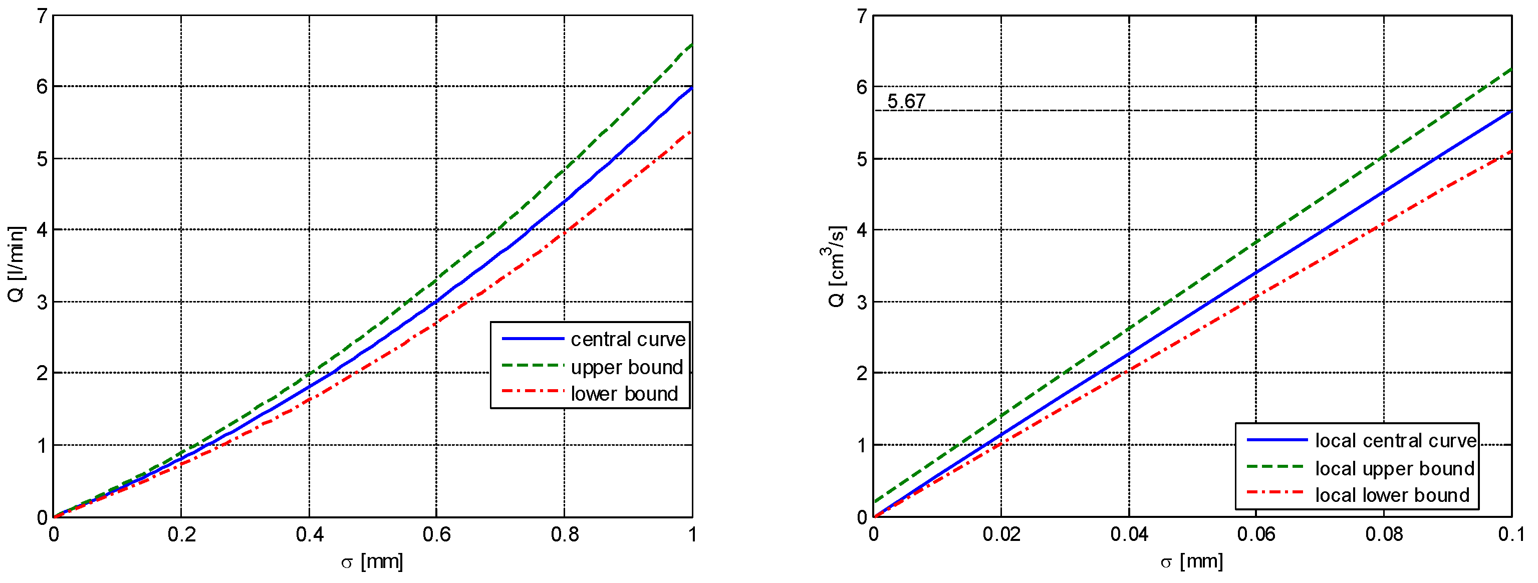
Overall Control Valve Characteristics
Flow  Q [L/min]—Control σ [mm]
σ [ 0 ; 1 ] mm
Local Control Valve Characteristics
Flow  Q [ cm 3 / s ] —Control σ [mm]
σ 0 ; 0.1 mm
central: Q c = σ 2.442076 σ + 3.543074 central: Q l = 56.7 σ
upper bound: Q u = 1.1 Q c upper bound: Q u = 0.2 + 60.41 σ
lower bound: Q l = 0.9 Q c lower bound: Q l = 51.07 σ
Table 2. Choices of the components of the feedback vector ( k p , k v , k a ) that ensure sufficient conditions for absolute stability of the hydraulic servomechanism system.
r p 2 + ω r 4 r a 2 4 ζ r r p r v / ω r 2 ω r 2 r p r a 4 ζ r ω r r v r a < 0
r a : = k A k a   ,       r v : = k A k v   ,       r p : = k A k p
k r = 1 / S ˜ ,   1 / ω r 2 = k c m / S S ˜ ,   2 ζ r / ω r = k l m / S S ˜ + k c f / S S ˜
k c = V c / 2 B ,   S ˜ = S + k l f / S
σ = k A u r e f k p x 1 k v x ˙ 1 k a x ¨ 1
choice of components inside the quadric of absolute stability (23); see Figure 1 for other notations;
condition derived from Barbashin–Krasovskii theorem
k v / k a 2 ζ r ω r k v ω r 2 / k p condition derived from V.M. Popov theorem
Table 3. Summary of hydraulic servo impedance and its role in flight controls flutter.
Imp i ω : = F s / z s = r d s + a 1 / s + a 2 a 1 = λ 2 k Q / S , a 2 = r d λ 3 k Q / E S + k Q p / S 2 , 1 / r d = 1 / E + k c / S 2 impedance definition, see (43), see Figure 5
Proposition 1 λ 2 k Q / S < k Q / E + k Q p / S S E / S 2 + k c E
note: impedance can also be defined for the electrohydraulic servomechanism [30].
see proof, see (48)
see graphs of the impedance function in the two cases
a 1 < a 2   flutter   damping
a 1 > a 2   flutter   enhancing
Table 4. Ratios δ i / δ m a x related to ω b and p.
δ 2 i / δ max i = 1 , p ¯ p = 5 ω b = 25 p = 5 ω b = 100 p = 10 ω b = 25 p = 10 ω b = 100
δ 2 / δ max 1111
δ 4 / δ max 0.05850.00370.24800.0155
δ 6 / δ max 000.01690
δ 8 / δ max 0000
Disclaimer/Publisher’s Note: The statements, opinions and data contained in all publications are solely those of the individual author(s) and contributor(s) and not of MDPI and/or the editor(s). MDPI and/or the editor(s) disclaim responsibility for any injury to people or property resulting from any ideas, methods, instructions or products referred to in the content.

