Disturbance-Resilient Flatness-Based Control for End-Effector Rehabilitation Robotics

Abstract

Robotic-assisted therapy is an increasingly vital approach for upper-limb rehabilitation, offering consistent, high-intensity training critical to neuroplastic recovery. However, current control strategies often lack robustness against uncertainties and external disturbances, limiting their efficacy in dynamic, real-world settings. Addressing this gap, this study proposes a novel control framework for the iTbot—a 2-DoF end-effector rehabilitation robot—by integrating differential flatness theory with a derivative-free Kalman filter (DFK). The objective is to achieve accurate and adaptive trajectory tracking in the presence of unmeasured dynamics and human–robot interaction forces. The control design reformulates the nonlinear joint-space dynamics into a 0-flat canonical form, enabling real-time computation of feedforward control laws based solely on flat outputs and their derivatives. Simultaneously, the DFK-based observer estimates external perturbations and unmeasured states without requiring derivative calculations, allowing for online disturbance compensation. Extensive simulations across nominal and disturbed conditions demonstrate that the proposed controller significantly outperforms conventional flatness-based control in tracking accuracy and robustness, as measured by reduced mean absolute error and standard deviation. Experimental validation under both simple and repetitive physiotherapy tasks confirms the system’s ability to maintain sub-millimeter Cartesian accuracy and sub-degree joint errors even amid dynamic perturbations. These results underscore the controller’s effectiveness in enabling compliant, safe, and disturbance-resilient rehabilitation, paving the way for broader deployment of robotic therapy in clinical and home-based environments.

1. Introduction

Robotic-assisted therapy has gained significant attention as an effective solution for restoring motor function in individuals with neuromuscular impairments, particularly those recovering from stroke and related conditions [1,2,3,4]. These systems enable high-intensity, repetitive, and goal-directed training, which is essential for promoting neuroplasticity and functional recovery. Unlike traditional physical therapy, where therapists manually guide patients through rehabilitation exercises, robotic systems provide structured assistance in passive, active, and assist-as-needed modes. Moreover, they facilitate precise monitoring of patient progress and allow for objective assessment of motor recovery [5,6]. Despite these advantages, significant challenges persist—especially in personalizing therapy for individual patients and scaling robotic systems for broader clinical and at-home applications [7].

Rehabilitation robots are typically categorized into two main types: exoskeleton and end-effector systems [7]. Exoskeleton robots are wearable devices designed to mimic the anatomical structure of the human arm, enabling multi-joint movement support for comprehensive rehabilitation [8,9,10,11,12]. While these robots can perform complex therapy routines, they tend to be bulky, expensive, and challenging to operate—factors that limit their suitability for home-based use [13]. In contrast, end-effector robots interact with users through a single physical interface, such as the wrist or forearm. Their mechanical simplicity, lower cost, and ease of deployment make them well-suited for non-clinical settings, including home rehabilitation [7]. Nonetheless, access to portable and consistent therapy remains limited, particularly for individuals facing logistical barriers to attending healthcare facilities.

To bridge this gap, we introduce iTbot, a two-degrees-of-freedom (2-DoF) end-effector-type therapeutic robot specifically designed for upper-limb rehabilitation. The iTbot is lightweight, compact, and capable of delivering therapy in both clinical and home environments. Its design emphasizes usability, portability, and adaptability, thereby expanding access to high-quality rehabilitation beyond traditional care settings.

A key challenge in robotic rehabilitation is the development of control strategies that facilitate accurate, safe, and robust interactions with users. For end-effector systems, the primary control goal is to achieve precise trajectory tracking during repetitive tasks such as elbow flexion and extension. However, this objective is complicated by actuator dynamics, system nonlinearities, external disturbances, and the inherently variable nature of human–robot interaction [9]. Several control methodologies have been proposed to address these issues. For example, backstepping control employs Lyapunov-based recursive design techniques to ensure stability, but it remains highly sensitive to modeling errors [14]. Other approaches, including fuzzy logic, neural networks, hybrid adaptive control, and machine learning, are capable of managing uncertainties [15,16,17,18]; however, they often entail high computational overhead, which complicates real-time implementation. Alternative strategies such as adaptive control [19], EMG-driven methods [20], admittance-based control [21], and sliding mode control [22] are also used but suffer from drawbacks like model dependency and noise sensitivity. Time Delay Estimation (TDE) provides a non-model-based compensation method for unmodeled dynamics [23], though it is often affected by noise and latency. Similarly, Extended Kalman Filters (EKFs) have been employed for state estimation [24,25], but the requirement for Jacobian-based linearization can compromise stability and increase implementation complexity.

A promising alternative lies in the flatness-based control paradigm introduced by Fliess and collaborators [12,26,27,28,29]. Differential flatness allows system states and control inputs of nonlinear systems to be expressed in terms of flat outputs and their derivatives, thereby significantly simplifying the control design process. Building upon our previous work [30], this paper presents a novel flatness-based control framework for the iTbot system. The proposed approach transforms the system dynamics into a 0-flat canonical form and integrates a derivative-free Kalman filter (DFK) to estimate unmeasured states and external disturbances in real-time. This combined method enhances tracking accuracy and robustness while maintaining computational efficiency, making it suitable for real-time application.

The main contributions can be summarized as follows:

• Development of a flatness-based control strategy specifically tailored to the iTbot platform, enabling precise and robust trajectory tracking.
• Derivation of a 0-flat canonical form of the system dynamics using differential geometric tools.
• Integration of a derivative-free Kalman filter for real-time estimation and rejection of external disturbances and unmeasured dynamics, without the need for derivative computations.
• Demonstration—through both simulations and real-time experiments—that the proposed method offers improved tracking performance and robustness under a variety of disturbance conditions, all with reduced computational load.

The remainder of this paper is structured as follows. Section 2 details the design and mechanical specifications of the iTbot system. Section 3 presents both the kinematic and dynamic modeling. In Section 4, the flatness-based control methodology is introduced alongside the disturbance estimation scheme employing DFK. Section 5 discusses the simulation-based comparative study, while Section 6 describes the experimental validation. Finally, Section 7 concludes the paper with a summary of findings and outlines directions for future research.

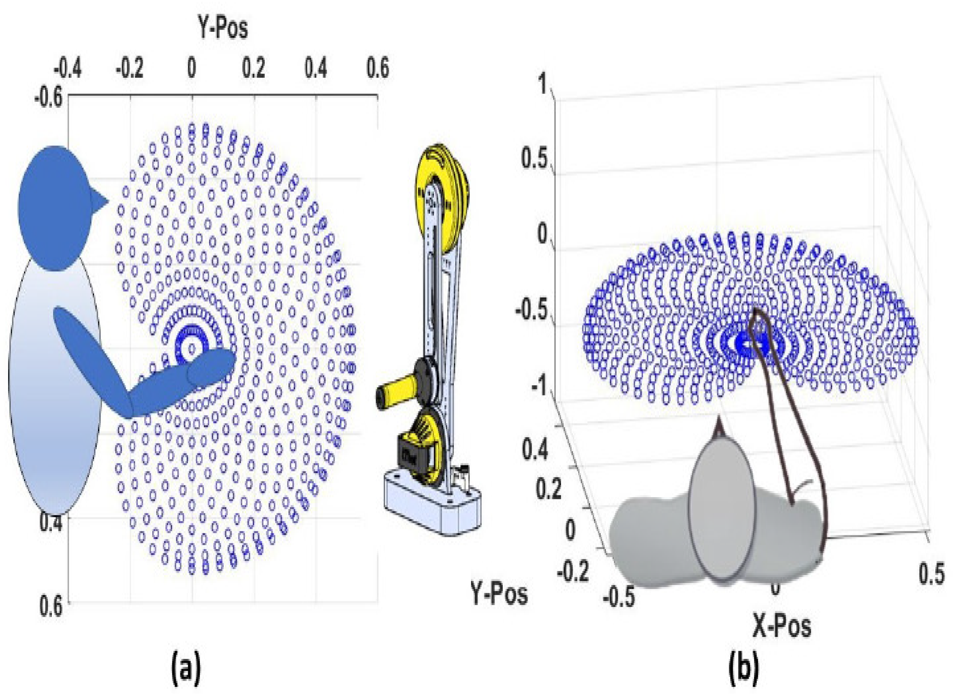
2. Mechanical Design of iTbot

The iTbot robot is designed to operate within a workspace that is accessible to humans, facilitating therapy throughout its entire range of motion. The mechanical design of the iTbot is deliberately simplified, yet it effectively supports robot-assisted rehabilitation, as shown in Figure 1. The robot’s structure comprises two linkages, Link-1 and Link-2, both mounted on a robust base. To enhance stability during experimental operations, the base of the iTbot is constructed from a heavy aluminum block. This block is formed from two aluminum components: one serves as the bottom of the robot, while the other functions as a mounting platform for the Motor-1 (Joint-1) assembly, as illustrated in Figure 1. Joint-1 (Motor-1) features a harmonic drive gear reducer, mounted directly onto the top of the base, with the motor positioned behind it using a custom-designed motor adapter. Link-1 is made of an aluminum segment that includes an integrated gear reducer, connecting directly to the output of the harmonic drive gear unit. In the Link-2 assembly, another aluminum component houses the second half of the Motor-2 wire spool holder. Joint-2 (Motor-2) consists of two interconnected links: Link-1 and Link-2.

At the end of the connection, an end effector holds both the force sensor and the handle. The handle is specifically tailored to fit the user’s hand profile; in our prototype, its design was based on the average hand size of two adult male laboratory members who participated in the development of the iTbot. This handle includes a base component that has been 3D-printed from polycarbonate plastic and is attached to the force sensor. An inner tube, equipped with mounting points for two bearings at either end, is then screwed into the base component to finalize the assembly.

Specification of the iTbot

The completed CAD model outlined in Section 2 was created by applying material properties to each component with SolidWorks software 2019. Table 1 provides a summary of the mechanical parameters derived for the iTbot. Figure 2 demonstrates that the iTbot offers a range of motion of 1.1 m along the X-axis. This robot was specifically designed to assist the motion of the human upper limb [32] within a workspace that accommodates individuals ranging in height from 1.21 to 1.82 m, allowing for both horizontal and vertical orientations. In Figure 2, the shaded area indicates the workspace coverage for a human arm, extending from 0.5 m to 0.66 m. Moreover, the iTbot’s base design facilitates installation in either a horizontal or vertical position, provided it is adequately anchored. Its symmetric design, paired with asymmetric joint ranges of motion, makes the robot suitable for use by both left- and right-handed individuals.

Figure 2. Reachable workspace of the upper limb under (a) vertical and (b) horizontal arrangements [31].

Figure 2. Reachable workspace of the upper limb under (a) vertical and (b) horizontal arrangements [31].

Table 1. Mechanical parameters of iTbot estimated from CAD model [31].

Joint Parameters
Item	Joint-1	Joint-2
Joint range of motion (degrees)	±85°	±180°
Link Parameters
Mass (Kg)	1.79	0.65
Location of the center of gravity in link frame (m)	Center of gravity of link 1 in frame {1}, see Figure 3 $X_1$ = 0.26, $Y_1$ = 0.00, $Z_1$ = 0.00	Center of gravity of link 2 in frame {2}, see Figure 3 $X_2$ = 0.15, $Y_2$ = 0.00, $Z_2$ = 0.02
Robot Properties
Mass (Kg)	6.67 (3.2 without base)
Maximum Horizontal reach (m)	±0.55
Maximum Vertical reach (m)	+0.1 to +0.55

Table 1. Mechanical parameters of iTbot estimated from CAD model [31].

Joint Parameters
Item	Joint-1	Joint-2
Joint range of motion (degrees)	±85°	±180°
Link Parameters
Mass (Kg)	1.79	0.65
Location of the center of gravity in link frame (m)	Center of gravity of link 1 in frame {1}, see Figure 3 $X_1$ = 0.26, $Y_1$ = 0.00, $Z_1$ = 0.00	Center of gravity of link 2 in frame {2}, see Figure 3 $X_2$ = 0.15, $Y_2$ = 0.00, $Z_2$ = 0.02
Robot Properties
Mass (Kg)	6.67 (3.2 without base)
Maximum Horizontal reach (m)	±0.55
Maximum Vertical reach (m)	+0.1 to +0.55

Figure 3. Coordinate frame assignment for the 2-DoF iTbot [31].

Figure 3. Coordinate frame assignment for the 2-DoF iTbot [31].

3. Kinematics and Mathematical Model of iTbot

The kinematic model of the iTbot employs the modified Denavit–Hartenberg (DH) notation [31]. As depicted in Figure 3, only two joint angles are actively controlled during rehabilitation training. Each link in the robot’s structure has an associated coordinate frame (link frame) that specifies its position concerning adjacent links. The DH parameters are determined by assigning coordinate frames that link one axis of rotation to the next. Frame 1 is associated with Joint 1, Frame 2 corresponds to Joint 2, and Frame 3 is designated for the iTbot’s end-effector. Frame 0 acts as the fixed reference frame, aligned with the world (base) frame. The modified DH parameters, which describe the spatial relationships of the link frames (shown in Figure 3), are summarized in

Table 2. The modified Denavit–Hartenberg (DH).

Joint (i)	${\mathit{\alpha }}_{\mathit{i}-1}$	${\mathit{d}}_{\mathit{i}}$	${\mathit{a}}_{\mathit{i}-1}$	${\mathit{\theta }}_{\mathit{i}}$
1	0	0	0	${\theta }_1+{\displaystyle \frac{\pi }{2}}$
2	0	0	$l_1$	${\theta }_2+\pi$
3	0	0	$l_2$	0

. Additionally, integrating the DH parameters, we obtain the homogeneous transformation matrix, which defines the positions and orientations of the reference frames relative to the fixed base frame.

In Table 2, ${\alpha }_{i-1}$ denotes the link twist, $a_{i-1}$ is the link length, $d_i$ represents the link offset, and ${\theta }_i$ is the joint angle.

Dynamics of the iTbot

The dynamic behavior of the iTbot is examined using the iterative Newton–Euler formulation, as shown in Figure 4 [33]. This approach allows for precise simulation of joint movements in experiments that utilize nonlinear control strategies.

The dynamic model of the iTbot, expressed in joint space, is illustrated below:

$$M\left(\theta \right)\ddot{\theta }+\mathcal{C}(\theta ,\dot{\theta })\dot{\theta }+G_r\left(\theta \right)+{\xi }_{dis}=\tau$$

(1)

where $\theta \in {\mathbb{R}}^2$ denotes the vector of generalized coordinates. $M\left(\theta \right)\in {\mathbb{R}}^{2\times 2}$ represents the symmetric positive-definite inertia matrix, $\mathcal{C}(\theta ,\dot{\theta })\dot{\theta }\in {\mathbb{R}}^2$ accounts for Coriolis and centrifugal forces, and $G_r\left(\theta \right)\in {\mathbb{R}}^2$ denotes the gravity vector. $\tau \in {\mathbb{R}}^2$ represents the torque input vector, while ${\xi }_{dis}\in {\mathbb{R}}^2$ incorporates external disturbances. Furthermore, it is important to note that ${\xi }_{dis}=J^T{F}_e$, where $J\in {\mathbb{R}}^{6\times 2}$ is the Jacobian matrix and $F_e\in {\mathbb{R}}^{6\times 1}$ denotes the contact force between the human and the robot.

The dynamic model presented in Equation (1) can be transformed into a state-space representation by incorporating the variables $x=\theta$ and $\dot{x}=\dot{\theta }$. This results in the following system:

$$\dot{x}=F(x,\dot{x})+G\left(x\right)u$$

(2)

where:

• $u=\tau$ is the control input (torque),
• $G\left(x\right)=G=M^{-1}\left(\theta \right)$ is the inverse of the inertia matrix,
• $F(x,\dot{x})=M^{-1}\left(\theta \right)\left[-\mathcal{C}(\theta ,\dot{\theta })\dot{\theta }-G_r\left(\theta \right)-{\xi }_{dis}(\theta ,\dot{\theta })\right]$ represents the system dynamics including nonlinearities and disturbances.

4. Control Design

It has been shown that the robot model, as described in Equation (2), is affected by uncertainties and external disturbances. The main objective is to develop a robust controller capable of supporting physical therapy movements. This will be accomplished through the use of a flat controller along with estimation techniques. The approach includes two essential strategies: the first takes advantage of the flatness property applicable to a certain class of dynamic systems, and the second employs the derivative-free Kalman (DFK) method.

4.1. Notation

Firstly, the following are presented [28]:

Definition 1. 

The Lie derivative is defined as the derivative of γ, with respect to the vector field F given by the following: $L_F\gamma ={\displaystyle \frac{\partial \gamma }{\partial x}}F\left(x\right)$. $L_F^0\gamma =\gamma$ for $i=0,$ and for $i=1,2,...$ we have $L_F^i\gamma =L_F{L}_F^{i-1}\gamma ={\displaystyle \frac{\partial L_F^{i-1}\gamma }{\partial x}}F\left(x\right)$.

Definition 2. 

The Lie Bracket of the two vector fields F and G, denoted as $a{d}_{F}G$ or $[F,G]\left(x\right)$, is defined as $[F,G]\left(x\right)={\displaystyle \frac{\partial G}{\partial x}}F-{\displaystyle \frac{\partial F}{\partial x}}G$. Additionally, we have $a{d}_F^{0}G=G\left(x\right)$ and $a{d}_F^{i}G=[F,a{d}_F^{i-1}G]$.

4.2. The Differential Geometric Approach

Let us start by defining the flatness property for a dynamic system that includes a control input described as follows:

$$\dot{x}=F\left(x\right)+\sum _{i=1}^m{G}_i\left(x\right)u_i$$

(3)

where x represents the state vector defined on $\mathcal{X}\subseteq {\Re }^n$, u is the input vector defined on $U\subseteq {\Re }^m$ while F, G are the vector fields defined on $\mathcal{X}\times U.$

Definition 3. 

A system described by Equation (3) is considered differentially flat if there are γ variables $\gamma \in {\Re }^m$, known as flat outputs $\gamma =({\gamma }_1,\dots ,{\gamma }_m)$, that satisfy the following condition:

1. 

γ is written as function of the state vector x, the control input vector u and its time derivatives $u^i$: $\gamma =h(x,u,\dot{u},\dots ,u^{\left(r_1\right)})$.

2. 

The components of the state vector x can be expressed from the flat output γ and its time derivatives: $x=\phi (\gamma ,\dot{\gamma },\dots ,{\gamma }^{\left(r_2\right)})$.

3. 

The components of the input vector u can be expressed from the flat output and its time derivatives: $u=y(\gamma ,\dot{\gamma },\dots ,{\gamma }^{(r_2+1)})$, where $h,\phi ,$ and y are smooth functions.

Let $G\left(x\right)=[G_1\left(x\right),\dots ,G_m\left(x\right)]$ denote a set of vector fields. We assume that this set has a rank of m.

The flat system is characterized by flat outputs, where all control inputs and state vectors are defined in relation to these output variables and a limited number of their derivatives. For a specific class of differentially flat systems, in this work we have only $\gamma =h\left(x\right)$ considered in (1) of Definition (3), which means that these systems are called 0-flat.

It demonstrates that dynamic affine systems with a co-dimension of 1, possessing n states and $n-1$ inputs, are controllable if and only if these systems are 0-flat [34].

One of the primary objectives of this work is to apply the properties of differential flatness. Once the system is demonstrated to be flat, it can undergo a transformation into the proposed 0-flat normal form, where geometric conditions are adequately provided. Similarly, this procedure yields an algorithm for computing the flat outputs. Additionally, a dynamic system (3) that has n states and m inputs is classified as having co-dimension 2 when the difference between n and m equals 2.

4.3. 0-Flat Form for Co-Dimension 2 System

The suggested canonical normal form for co-dimension 2 dynamic systems is presented as follows:

Proposition 1. 

A dynamic system of co-dimension 2 is considered 0-flat if it can be expressed in the following:

$$\left\{\begin{array}{ccc}{\dot{\zeta }}_{1,1}\hfill & =\hfill & {\zeta }_{1,2}+\sum _{i=3}^{m=n-2}{\phi }_{1,1}^i\left(\zeta \right)u_i\hfill \\ {\dot{\zeta }}_{1,2}\hfill & =\hfill & {\beta }_{1,2}\left(\zeta \right)+{\phi }_{1,2}^1\left(\zeta \right)u_1+{\phi }_{1,2}^2\left(\zeta \right)u_2+\dots +{\phi }_{1,2}^m\left(\zeta \right)u_m\hfill \\ {\dot{\zeta }}_{2,1}\hfill & =\hfill & {\zeta }_{2,2}+\sum _{i=3}^{m=n-2}{\phi }_{2,1}^i\left(\zeta \right)u_i\hfill \\ {\dot{\zeta }}_{2,2}\hfill & =\hfill & {\beta }_{2,2}\left(\zeta \right)+{\phi }_{2,2}^1\left(\zeta \right)u_1+{\phi }_{2,2}^2\left(\zeta \right)u_2+\dots +{\phi }_{2,2}^m\left(\zeta \right)u_m\hfill \\ \dots \hfill & =\hfill & \dots \dots \dots \dots \hfill \\ {\dot{\zeta }}_{j,1}\hfill & =\hfill & {\beta }_{j,1}\left(\zeta \right)+\sum _{i=3,i\ne j}^{m=n-2}{\phi }_{j,1}^i\left(\zeta \right)u_i\hfill \end{array}\right.$$

(4)

The flat outputs are represented as: ${\gamma }_j={\left({\zeta }_{j,1}\right)}_{1\le j\le m=n-2}$, and $\zeta =({\left({\zeta }_{j,1}\right)}_{1\le j\le m=n-2},{\zeta }_{1,2},{\zeta }_{2,2})$ is the updated vector of the system.

Proof of Proposition 1. 

Now, we will demonstrate that the previously described system dynamics, represented in the proposed normal form of Equation (4), are 0-flat. We will examine the following m equations:

$$\begin{array}{c}\hfill T_1={\dot{\zeta }}_{1,1}-{\zeta }_{1,2}-\sum _{i=3}^{m=n-2}{\phi }_{1,1}^i\left(\zeta \right)u_i=0\end{array}$$

(5)

$$\begin{array}{c}\hfill T_2={\dot{\zeta }}_{2,1}-{\zeta }_{2,2}-\sum _{i=3}^{m=n-2}{\phi }_{2,1}^i\left(\zeta \right)u_i=0\\ \hfill \dots \dots \dots \dots \dots \dots \dots \dots \dots \end{array}$$

(6)

$$\begin{array}{c}\hfill T_j={\dot{\zeta }}_{j,1}-{\beta }_{j,1}\left(\zeta \right)-\sum _{i=3,i\ne j}^{m=n-2}{\phi }_{j,1}^i\left(\zeta \right)u_i=0\end{array}$$

(7)

where $(3\le j\le m=n-2).$

Consider the vector $\eta =({\zeta }_{1,2},{\zeta }_{2,2},u_1,u_2,...,u_{m=n-2})$, which consists of the unknown system variables. We will use this vector later to compute the partial derivative of $T_1,T_2,...,T_{m=n-2}$ as follows:

$$\begin{array}{c}\hfill {\displaystyle \frac{\partial (T_1,T_2,...,T_m)}{\partial \eta }}=-I_m+\rho \left(\eta \right)\end{array}$$

(8)

where $I_m$ denotes the $(m\times m)$ identity matrix, and $\rho \left(\eta \right)$ comprises terms that are of order one with respect to the $\eta$ variables. Using the equations provided (5)–(7), and recognizing that the partial derivative ${\displaystyle \frac{\partial (T_1,...,T_m)}{\partial \eta }}$ is locally invertible, we can apply the implicit function theorem. This enables us to conclude that there exist two functions ${\lambda }_k\left(\right)$ and ${\delta }_k\left(\right)$ such that:

$$\begin{array}{c}\hfill {\zeta }_{k,2}={\lambda }_k({\gamma }_j,{\dot{\gamma }}_j,j=1,.,n-2,k=1:2)\end{array}$$

(9)

$$\begin{array}{c}\hfill u_k={\delta }_k({\gamma }_j,{\dot{\gamma }}_j,j=1,.,n-2,k=3:m)\end{array}$$

(10)

Next, by substituting Equations (9) and (10) into Equation (4), we can derive the unknown system variables, which are the control inputs $(u_1$, $u_2$, and $u_3,\dots u_m)$. These inputs are expressed in terms of the flat outputs ${({\gamma }_j,{\dot{\gamma }}_j)}_{(j=1:m=n-2)}$ and their second time derivative $\left({\gamma }_1^2\right),\left({\gamma }_2^2\right),\dots {\gamma }_m^2$.

Thus, the state vector and control inputs can be represented as functions of flat outputs $\gamma$ and their successive time derivatives. This indicates that dynamic systems with co-dimension 2 exhibit differential flatness properties. Consequently, Proposition 1 has been proven. □

4.4. Geometrical Background

This section focuses on outlining the geometrically sufficient conditions required for our dynamic system to be transformed into the previously proposed flatness normal form, in which the outputs are flat.

Next, we assume that the controllability distribution, represented by Δ, has a dimension of n such that:

$$\Delta =span\{G_1,G_2,...,G_{n-2},a{d}_F{G}_i,a{d}_F{G}_j\}$$

(11)

where $a{d}_F{G}_i,a{d}_F{G}_j$ denotes Lie brackets.

It is important to recognize that $G_i,G_j\in \{G_1,G_2,G_3,G_4,...,G_{n-2}\}$. For ease of discussion, the vector fields $G_i$ and $G_j$ can be expressed as $G_i=G_1$ and $G_j=G_2$, respectively, without losing generality.

Theorem 1. 

The transformation of the system of Equation (3) into the proposed 0-flat form occurs through a change in coordinates if and only if the distribution $\overline{\Delta }=\{G_1,G_2\}\subseteq \Delta$ is involutive.

Proof of Theorem 1. 

$\Delta$ is considered a nonsingular distribution generated by the set of vector fields. If the involutive condition $\overline{\Delta }=\{G_1,G_2\}\subseteq \Delta$ is verified, then Frobenius theorem [35] states that there exist $m=n-2$ independent state functions $({\gamma }_i\left(x\right)={\zeta }_{i,1})$${(}_{1\le i\le m=n-2})$ such that:

$$\begin{array}{c}\hfill \overline{\Delta }=\bigcap _{i=1}^{m}kerd{\gamma }_i\end{array}$$

(12)

where $kerd{\gamma }_i$ denotes the kernel of the differential of the function ${\gamma }_i$. Next, we introduce the following Lie brackets:

$$\begin{array}{c}\hfill L_{[G_k,F]}{\gamma }_k\ne 0,fork=1,2\end{array}$$

(13)

$$\begin{array}{c}\hfill L_{G_k}{\gamma }_k=0,fork=1:2\end{array}$$

(14)

As a result, the new state vector $\zeta$ is created based on the following Equations (13) and (14), detailed as follows:

$$({\zeta }_{i,1}={\gamma }_i\left(x\right),{(}_{1\le i\le m=n-2})),and({\zeta }_{1,2}=L_F{\zeta }_{1,1},{\zeta }_{2,2}=L_F{\zeta }_{2,1})$$

(15)

Now, if we consider ${\zeta }_{1,1}={\gamma }_1\left(x\right)$, ${\zeta }_{1,2}=L_F{\gamma }_1\left(x\right)$, the derivation of ${\dot{\zeta }}_{1,1}$ results in

$${\dot{\zeta }}_{1,1}={\zeta }_{1,2}+\sum _{i=3}^{m=n-2}L{G}_i{\gamma }_1\left(x\right)u_i$$

(16)

Thus, we can put ${\phi }_{1,1}^i\left(\zeta \right)=L{G}_i{\gamma }_1\left(x\right)$ and ${\phi }_{2,1}^i\left(\zeta \right)=L{G}_i{\gamma }_2\left(x\right)$, while the other variables: $({\phi }_{1,2}^1\left(\zeta \right),{\phi }_{1,2}^2\left(\zeta \right)$ …${\phi }_{1,2}^m\left(\zeta \right))$ and $({\phi }_{2,2}^1\left(\zeta \right),{\phi }_{2,2}^2\left(\zeta \right)$ …${\phi }_{2,2}^m\left(\zeta \right))$ are also defined in Equation (4) by the derivation of the variable ${\zeta }_{1,2}$ and ${\zeta }_{2,2}$.

Now, we can obtain the proposed flatness normal form (4) by applying the same procedure of successive derivations to all other selected outputs of the system. □

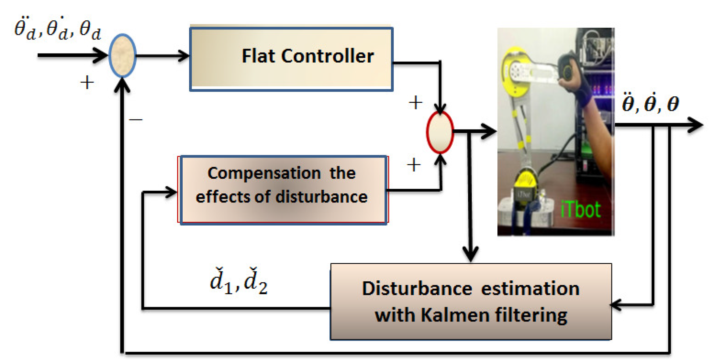
4.5. Design of a Flatness Based Controller for iTbot’s Robot System

To demonstrate that iTbot’s dynamic model (2) is differentially flat, we will utilize the following transformations to achieve a proposed 0-flat form (4). Let us begin by rewriting the robot’s dynamic model (2) in this format:

$$\dot{x}=F\left(x\right)+\sum _{i=1}^{m=n-2}{G}_i\left(x\right)u_i$$

(17)

where $x^T=\left[{\theta }_1{\theta }_2\dot{{\theta }_1}\dot{{\theta }_2}\right]=\left[x_1{x}_2{x}_3{x}_4\right]$ represents the state space vector of iTbot’s dynamic model, $u_i$ signifies the inputs, and $F\left(x\right)$ and $G_i\left(x\right)$ are smooth vector fields.

$$\begin{array}{cc}\hfill F\left(x\right)=& \left[\begin{array}{c}{x}_3\\ x_4\\ F_1\left(x\right)\\ F_2\left(x\right)\end{array}\right]\end{array}$$

(18)

with $F^{\prime }\left(x\right)={\left[F_1\left(x\right)F_2\left(x\right)\right]}^T$ where $F^{\prime }\left(x\right)=M^{-1}\left(x_1\right)[\tau -\mathcal{C}(x_1,x_2)x_2-G_r\left(x_1\right)-{\xi }_{dis}]$, and

$$\begin{array}{cc}\hfill G_i\left(x\right)=& \left[\begin{array}{c}0\\ 0\\ G_{i1}\left(x\right)\\ G_{i2}\left(x\right)\end{array}\right]\end{array}$$

(19)

where $i=n-2$.

Next, we will examine the controllability distribution defined by the following vector fields: $\Delta =span\{G_1,G_2,a{d}_F{G}_1,a{d}_F{G}_2\}$. In contrast, the dimension is consistently set to n = 4. Meanwhile, the distribution of dimensions $\overline{\Delta }=span\{G_1,G_2\}$ is 2.

Thus, when verifying the following Lie brackets, one finds that

$$\begin{array}{c}\hfill [G_i,G_j]\in \Delta \forall 1\le i,j\le n-2=m\end{array}$$

The distribution $\overline{\Delta }\in \Delta$ is involutive, which means the earlier condition stated in Theorem 1 is satisfied.

Next, we can also ensure the existence of $n-2$ smooth functions ${\gamma }_1,$${\gamma }_2$ that satisfy the following partial differential equations, as dictated by the Frobenius theorem:

$$\begin{array}{c}\hfill d{\gamma }_1\left(x\right).\overline{\Delta }=0\end{array}$$

(20)

$$\begin{array}{c}\hfill d{\gamma }_2\left(x\right).\overline{\Delta }=0\end{array}$$

(21)

Equations (20) and (21) written as:

$$\begin{array}{c}\hfill d{\gamma }_1\left(x\right)[G_1\left(x\right),G_2\left(x\right)]=0\end{array}$$

(22)

$$\begin{array}{c}\hfill d{\gamma }_2\left(x\right)[G_1\left(x\right),G_2\left(x\right)]=0\end{array}$$

(23)

From (20) and (21), we can conclude that for all $(x_1,x_2)$, it holds that:

$$\begin{array}{c}\hfill {\displaystyle \frac{\partial {\gamma }_i}{\partial x_j}}=0(i=1:2andj=3:4)\end{array}$$

(24)

As a result of the analysis presented above, we can describe ${\gamma }_1\left(x\right)$ and ${\gamma }_2\left(x\right)$ in the following manner:

$$\begin{array}{c}\hfill {\gamma }_1\left(x\right)=x_1={\zeta }_{1,1}\end{array}$$

(25)

$$\begin{array}{c}\hfill {\gamma }_2\left(x\right)=x_2={\zeta }_{2,1}\end{array}$$

(26)

where ${\zeta }_{1,1},$ and ${\zeta }_{2,1}$ represent the flat outputs generated by iTbot’s dynamic model.

The new state variables $\zeta$ of the system are created from the collection of flat outputs ${\zeta }_{1,1}$, ${\zeta }_{2,1}$, and 2, along with the additional variables: $\zeta =({\zeta }_{i,1}={\gamma }_i\left(x\right){,}_{1\le i\le 2})$ and ${\zeta }_{1,2}=L_F{\zeta }_{1,1},{\zeta }_{2,2}=L_F{\zeta }_{2,1}$.

The updated vector of the system is expressed as $\zeta =[{\zeta }_{1,1},{\zeta }_{1,2},{\zeta }_{2,1},{\zeta }_{2,2}]$.

The first equation in normal form (4) is derived from the derivative of the initial flat output ${\dot{\zeta }}_{1,1}$. Consequently, the derivatives of other variables, we can outline the triangular 0-flat form for a dynamic system of co-dimension 2 as follows:

$$\begin{array}{ccc}\hfill {\dot{\zeta }}_{1,1}& =& {\zeta }_{1,2}+\sum _{i=3}^{m=n-2}{\phi }_{1,1}^i\left(\zeta \right)u_i\hfill \\ \hfill {\dot{\zeta }}_{1,2}& =& {\beta }_{1,2}\left(\zeta \right)+{\phi }_{1,2}^1\left(\zeta \right)u_1+{\phi }_{1,2}^2\left(\zeta \right)u_2+{\tilde{d}}_1\hfill \\ \hfill {\dot{\zeta }}_{2,1}& =& {\zeta }_{2,2}+\sum _{i=3}^{m=n-2}{\phi }_{2,1}^i\left(\zeta \right)u_i\hfill \\ \hfill {\dot{\zeta }}_{2,2}& =& {\beta }_{2,2}\left(\zeta \right)+{\phi }_{2,2}^1\left(\zeta \right)u_1+{\phi }_{2,2}^2\left(\zeta \right)u_2+{\tilde{d}}_2\hfill \end{array}$$

(27)

In the normal flat form, the variables ${\tilde{d}}_1$ and ${\tilde{d}}_2$ represent external disturbances, appearing in the second and fourth rows, respectively.

Furthermore, all state variables and the control input of the iTbot model are defined as functions of the flat output and its derivatives. As a result, the studied system is considered to be differentially 0-flat. Now, we can establish the expressions for the appropriate control inputs $u_1$ and $u_2$ based on the second and fourth equations from the triangular form (27). Consequently, ${\vartheta }_i$$(i=1:2)$ defines two new control inputs that are created using the specified flat outputs ${\zeta }_{1,1}$ and ${\zeta }_{2,1}$, along with their derivatives, aligned with the desired values of the designated reference trajectories. ${\zeta }^{ref},{\dot{\zeta }}^{ref},{\ddot{\zeta }}^{ref}$ such that:

$$\begin{array}{c}\hfill {\vartheta }_i={\ddot{\zeta }}_{i,1}^{ref}+k_{d_{i,1}}({\dot{\zeta }}_{i,1}^{ref}-{\dot{\zeta }}_{i,1})+k_{p_{i,1}}({\zeta }_{i,1}^{ref}-{\zeta }_{i,1}){, }_{i=1:2}\end{array}$$

(28)

where $k_{d_{i,1}}$ and $k_{p_{i,1}}$ are selected control gains that ensure the asymptotic elimination of the tracking errors, $li{m}_{t\to \infty }{e}_i\left(t\right)=0$.

In the following section, we will estimate the external disturbances ${\tilde{d}}_i$ that influence the robotic model, as well as the disturbance terms related to parametric uncertainty. This will be accomplished simultaneously using the derivative-free Kalman Filtering (DFK) method.

4.6. Filtering Kalman for Dynamical Systems

It is assumed that the dynamical system can be represented as a discrete-time state model ([36,37,38]) in the following manner:

$$\begin{array}{cc}\hfill x(k+1)& =A\left(k\right)x\left(k\right)+J\left(k\right)u\left(k\right)+\omega \left(k\right)\hfill \\ \hfill z\left(k\right)& =Cx\left(k\right)+\nu \left(k\right)\hfill \end{array}$$

(29)

where $x\in {\Re }^{m\times 1}$ represents the system’s state vector, $z\in {\Re }^{p\times 1}$ is the system’s output. $\omega \left(k\right)$ and $\nu \left(k\right)$ signify the process noise, which is uncorrelated with the respective covariance matrices $\check{Q}$ and $\check{R}$. A is a $(m\times m)$ real matrix, J is the control input matrix, while C is a $p\times m$ matrix consisting of real numbers. The structure of the discrete-time Kalman filter equations is organized as follows:

$$\begin{array}{cc}\hfill \widehat{x}\left(k\right)& ={\widehat{z}}^{-}\left(k\right)+\check{K_F}\left(k\right)[x\left(k\right)-C{\widehat{z}}^{-}\left(k\right)]\hfill \\ \hfill \check{P}\left(k\right)& ={\check{P}}^{-}\left(k\right)-\check{K_F}\left(k\right)C{\check{P}}^{-}\left(k\right)\hfill \end{array}$$

(30)

The initial stage is referred to as the time update or prediction stage, which provides estimates $x\left(k\right)$ prior to the availability of the output measurement $z\left(k\right)$ (resulting in an a priori estimate).

$$\begin{array}{cc}\hfill {\check{K}}_F\left(k\right)& ={\check{P}}^{-1}\left(k\right)C^T{[C.{\check{P}}^{-1}\left(k\right)C^T+\check{R}]}^{-1}\hfill \\ \hfill {\check{P}}^{-}(k+1)& =A\left(k\right)\check{P}\left(k\right)A^T\left(k\right)+\check{Q}\left(k\right)\hfill \\ \hfill {\widehat{x}}^{-}(k+1)& =A\left(k\right)\widehat{x}\left(k\right)+J\left(k\right)u\left(k\right)\hfill \end{array}$$

(31)

$x\left(k\right)$ is estimated during the second part, known as the measurement update or correction stage, after $z\left(k\right)$ has been made available (a posteriori estimate).

4.7. Disturbances Compensation Using (DFK) Derivative-Free Kalman Filtering

The controller described here is capable of providing highly accurate tracking of the desired trajectory while also exhibiting robust performance in the face of disturbances. These disturbances may arise from parametric uncertainties, variations, or external factors. To effectively counter these disturbances and uncertainties, we can incorporate derivative-free Kalman filtering (DFK) into the flat-based feedback controller loop, as illustrated in Figure 5.

In Section 4.5, we showed that the nonlinear model of iTbot’s robot, as outlined in Equation (17), is differentially 0-flat. This was established by converting it into a triangular 0-flat normal form, accomplished through Equation (27).

In the dynamic model of the robot expressed in a triangular 0-flat normal form, the stabilizing feedback controller is represented as follows:

$$\begin{array}{c}\hfill {\vartheta }_1={\ddot{\zeta }}_{1,1}^{ref}+k_{d_{1,1}}({\dot{\zeta }}_{1,1}^{ref}-{\dot{\zeta }}_{1,1})+k_{p_{1,1}}({\zeta }_{1,1}^{ref}-{\zeta }_{1,1})\\ \hfill {\vartheta }_2={\ddot{\zeta }}_{2,1}^{ref}+k_{d_{2,1}}({\dot{\zeta }}_{2,1}^{ref}-{\dot{\zeta }}_{2,1})+k_{p_{2,1}}({\zeta }_{2,1}^{ref}-{\zeta }_{2,1})\end{array}$$

(32)

The dynamics of the tracking error are obtained as follows:

$$\begin{array}{c}\hfill ({\ddot{\zeta }}_{1,1}^{ref}-{\ddot{\zeta }}_{1,1})+k_{d_{1,1}}({\dot{\zeta }}_{1,1}^{ref}-{\dot{\zeta }}_{1,1})+k_{p_{1,1}}({\zeta }_{1,1}^{ref}-{\zeta }_{1,1})=0\\ \hfill ({\ddot{\zeta }}_{2,1}^{ref}-{\ddot{\zeta }}_{2,1})+k_{d_{2,1}}({\dot{\zeta }}_{2,1}^{ref}-{\dot{\zeta }}_{2,1})+k_{p_{2,1}}({\zeta }_{2,1}^{ref}-{\zeta }_{2,1})=0\end{array}$$

(33)

Assuming that the effects of both modeling uncertainty and external perturbations on the iTbot’s robot are represented as additive disturbance inputs $({\tilde{d}}_1$, ${\tilde{d}}_2)$, and these disturbances are incorporated into the initial nonlinear model of the iTbot as follows:

$$\begin{array}{ccc}\hfill {\ddot{x}}_1& =& {\vartheta }_1+{\tilde{d}}_1\hfill \\ \hfill {\ddot{x}}_2& =& {\vartheta }_2+{\tilde{d}}_2\hfill \end{array}$$

(34)

or in the second and fourth rows of the normal flat form after transformation (27) such that:

$$\begin{array}{ccc}\hfill {\ddot{\zeta }}_{1,1}& =& {\beta }_{1,2}\left(\zeta \right)+{\phi }_{1,2}^1\left(\zeta \right)u_1+{\phi }_{1,2}^2\left(\zeta \right)u_2+{\tilde{d}}_1\hfill \\ \hfill {\ddot{\zeta }}_{2,1}& =& {\beta }_{2,2}\left(\zeta \right)+{\phi }_{2,2}^1\left(\zeta \right)u_1+{\phi }_{2,2}^2\left(\zeta \right)u_2+{\tilde{d}}_2\hfill \end{array}$$

(35)

and by establishing the new control inputs

$$\begin{array}{ccc}\hfill {\vartheta }_1& =& {\beta }_{1,2}\left(\zeta \right)+{\phi }_{1,2}^1\left(\zeta \right)u_1+{\phi }_{1,2}^2\left(\zeta \right)u_2\hfill \\ \hfill {\vartheta }_2& =& {\beta }_{2,2}\left(\zeta \right)+{\phi }_{2,2}^1\left(\zeta \right)u_1+{\phi }_{2,2}^2\left(\zeta \right)u_2\hfill \end{array}$$

(36)

The dynamics can be expressed as follows:

$$\begin{array}{c}\hfill {\ddot{\zeta }}_{1,1}={\vartheta }_1+{\tilde{d}}_1\\ \hfill {\ddot{\zeta }}_{2,1}={\vartheta }_1+{\tilde{d}}_2\end{array}$$

(37)

The behavior of the disturbance terms is characterized by the time derivatives of the disturbance variables, extending up to order n. [39,40]. These terms are formatted as follows for (n = 2):

$$\begin{array}{c}\hfill {\ddot{\tilde{d}}}_1=f_{{\tilde{d}}_1}\\ \hfill {\ddot{\tilde{d}}}_2=f_{{\tilde{d}}_2}\end{array}$$

(38)

To account for the additional state variables, disturbance inputs, and their time derivatives, we expand the system’s state vector. The new state variables of the system are then determined as follows: ${\zeta }_e={[{\zeta }_{1,1}{\zeta }_{1,2}{\zeta }_{2,1}{\zeta }_{2,2}{\zeta }_{{\tilde{d}}_{1,1}}{\zeta }_{{\tilde{d}}_{1,2}}{\zeta }_{{\tilde{d}}_{2,2}},{\zeta }_{{\tilde{d}}_{2,2}}]}^T$.

Now, we can express the dynamics of the extended state space model of the robot as follows: ${\zeta }_{1,1}=x_1,{\zeta }_{1,2}={\dot{x}}_1,{\zeta }_{2,1}=x_2,{\zeta }_{2,2}={\dot{x}}_2,{\zeta }_{{\tilde{d}}_{1,1}}={\tilde{d}}_1,{\zeta }_{{\tilde{d}}_{1,2}}={\dot{\tilde{d}}}_1,{\zeta }_{{\tilde{d}}_{2,1}}={\tilde{d}}_2,{\zeta }_{{\tilde{d}}_{2,2}}={\dot{\tilde{d}}}_2$.

Therefore, the structure of the extended state space of iTbot’s robot represented by its normal flat form (27) of co-dimension 2 can be written as follows:

$$\begin{array}{c}\hfill {\dot{\zeta }}_e=\left(A_e\right){\zeta }_e+\left(B_e\right)\vartheta \\ \hfill {\zeta }_e^{me}=\left(Ce\right){\zeta }_e\end{array}$$

(39)

A state estimator has been created for the extended state-space representation of the system:

$$\begin{array}{c}\hfill {\dot{\widehat{\zeta }}}_e=\left(A_e\right){\widehat{\zeta }}_e+\left(B_e\right)\vartheta +K_f({\zeta }_e^{me}-C_e{\widehat{\zeta }}_e)\\ \hfill {\zeta }_e^{me}=C_e{\zeta }_e\end{array}$$

(40)

where

$$Ae=\left(\begin{array}{cccccccc}0& 1& 0& 0& 0& 0& 0& 0\\ 0& 0& 0& 0& 1& 0& 0& 0\\ 0& 0& 0& 1& 0& 0& 0& 0\\ 0& 0& 0& 0& 0& 0& 1& 0\\ 0& 0& 0& 0& 0& 1& 0& 0\\ 0& 0& 0& 0& 0& 0& 0& 0\\ 0& 0& 0& 0& 0& 0& 0& 1\\ 0& 0& 0& 0& 0& 0& 0& 0\end{array}\right)$$

(41)

and

$$B_e=\left(\begin{array}{cc}0& 0\\ 1& 0\\ 0& 0\\ 0& 1\\ 0& 0\\ 0& 0\\ 0& 0\\ 0& 0\end{array}\right),C_e=\left(\begin{array}{cccccccc}1& 0& 0& 0& 0& 0& 0& 0\\ 0& 0& 1& 0& 0& 0& 0& 0\end{array}\right)$$

(42)

The estimation of the unmeasurable elements of the state vector, as well as the disturbance inputs and their derivatives, is performed using the Kalman Filter recursion, which is outlined in the following step:

• First step (measurement update):

  $$\begin{array}{c}\hfill {\check{K}}_F\left(k\right)={\check{P}}^{-}\left(k\right)C_{di}^T{[C_{di}{\check{P}}^{-}\left(k\right)C_{di}^T+\check{R}]}^{-1}\\ \hfill {\widehat{\zeta }}_e\left(k\right)={\widehat{\zeta }}_e^{-}\left(k\right)+{\check{K}}_F\left(k\right)[{\zeta }_e^{me}\left(k\right)-C_{di}{\widehat{\zeta }}_e^{-}\left(k\right)]\\ \hfill \check{P}\left(k\right)={\check{P}}^{-}\left(k\right)-K_F\left(k\right)C_{di}{\check{P}}^{-}\left(k\right)\end{array}$$

  (43)
• Second step (time update):

  $$\begin{array}{c}\hfill {\check{P}}^{-}(k+1)=A_{di}\left(k\right)\check{P}\left(k\right)A_{di}^T\left(k\right)+\check{Q}\left(k\right)\\ \hfill {\widehat{\zeta }}_e^{-}(k+1)=A_{di}\left(k\right){\widehat{\zeta }}_e\left(k\right)+B_{di}\left(k\right)\vartheta \left(k\right)\end{array}$$

  (44)
  $A_{di}, B_{di}$ and $C_{di}$ are defined as the discrete-time equivalents of the previous matrices $A_e, B_e$ and $C_e.$

As a result, the new control input for the iTbot’s robot has been adjusted to account for the effects of disturbances, expressed as follows:

$$\begin{array}{c}\hfill {\vartheta }_1={\ddot{\zeta }}_{1,1}^{ref}+k_{d_{1,1}}({\dot{\zeta }}_{1,1}^{ref}-{\dot{\zeta }}_{1,1})+k_{p_{1,1}}({\zeta }_{1,1}^{ref}-{\zeta }_{1,1})-{\widehat{\zeta }}_{{\tilde{d}}_{1,1}}\\ \hfill {\vartheta }_2={\ddot{\zeta }}_{2,1}^{ref}+k_{d_{2,1}}({\dot{\zeta }}_{2,1}-{\dot{\zeta }}_{2,1})+k_{p_{2,1}}({\zeta }_{2,1}^{ref}-{\zeta }_{2,1})-{\widehat{\zeta }}_{{\tilde{d}}_{2,1}}\end{array}$$

(45)

The dynamics of tracking error for the closed-loop system can be described by the following equation:

$$\begin{array}{c}\hfill {\ddot{e}}_i+k_{d_i}{\dot{e}}_i+k_{p_i}{e}_i=0\end{array}$$

(46)

4.8. Stability Studies

In the following section, the Lyapunov function is used to demonstrate the asymptotic stability of the closed-loop system, which can be:

$$\begin{array}{c}\hfill {\ddot{e}}_i+k_{d_i}{\dot{e}}_i+k_{p_i}{e}_i=0\end{array}$$

(47)

Proposition 2. 

The dynamic model of the iTbot described earlier has been shown to be 0-flat, based on the principles of differential flatness theory (27). According to Equation (46), when the system operates in a closed-loop configuration using the two control inputs $u_1$ and $u_2$ from (27), it achieves global exponential stability. This stability is attained by selecting positive-definite diagonal gain matrices ($k_p$ and $k_d$). Moreover, the errors $e_i,{\dot{e}}_i$, along with the additive disturbance inputs ${\tilde{d}}_1$ and ${\tilde{d}}_2$, are kept within bounded limits.

Proof of Proposition 2. 

We introduce the following Lyapunov function:

$$V_l(e,\dot{e})=\sum _{i=1}^2{\displaystyle \frac{1}{2}}{k}_{p_i}{e}_i^2+\sum _{i=1}^2{\displaystyle \frac{1}{2}}{\dot{e}}_i^2$$

(48)

The derivative of $V_l$ can be expressed as:

$$\dot{V_l}(e,\dot{e})=\sum _{i=1}^2{k}_{p_i}{e}_i{\dot{e}}_i+\sum _{i=1}^2{\dot{e}}_i{\ddot{e}}_i$$

(49)

Substituting Equation (47) into Equation (49) yields:

$$\dot{V_l}(e,\dot{e})=\sum _{i=1}^2{k}_{p_i}{e}_i{\dot{e}}_i+\sum _{i=1}^2{\dot{e}}_i(-k_{d_i}{\dot{e}}_i-k_{p_i}{e}_i)$$

(50)

Simplifying results in:

$$\dot{V_l}(e,\dot{e})=\sum _{i=1}^2{k}_{p_i}{e}_i{\dot{e}}_i-\sum _{i=1}^2{k}_{d_i}{\dot{e}}_i^2-\sum _{i=1}^2{k}_{p_i}{e}_i{\dot{e}}_i$$

(51)

Therefore, we ultimately arrive at:

$$\dot{V_l}(e,\dot{e})=-\sum _{i=1}^2{k}_{d_i}{\dot{e}}_i^2\le 0$$

(52)

Then, by applying Barbalat’s lemma [41], we can confirm the global stability of the system. After differentiating Equation (52), we obtain:

$$\ddot{V_l}(e,\dot{e})=-2\sum _{i=1}^2{k}_{d_i}{\dot{e}}_i{\ddot{e}}_i$$

(53)

Since all gains $k_p$ and $k_d$ are positive, the state vector $\zeta$, ${\zeta }^{ref}$, and the additive disturbance ${\tilde{d}}_1$, ${\tilde{d}}_2$ are limited in scope. Similarly, the errors $e_i$, ${\dot{e}}_i$, and ${\ddot{e}}_i$ are also confined within certain bounds. Therefore, it can be concluded that ${\dot{V}}_l(e,\dot{e})$ is likewise bounded.

The derived $\dot{V}{(e,\dot{e})}_l$ exhibits uniform continuity. Given that the target trajectory ${\zeta }^{ref},\dot{{\zeta }^{ref}}$ and ${\ddot{\zeta }}^{ref}$ are also uniformly continuous, it follows that the errors $e_i$, ${\dot{e}}_i$, and ${\ddot{e}}_i$ are uniformly continuous as well. According to Barbalat’s lemma, $li{m}_{t\to \infty }\dot{V}{(e,\dot{e})}_l$=0, $li{m}_{t\to \infty }{e}_i=0$, and $li{m}_{t\to \infty }\dot{e_i}=0$. Under these conditions, the iTbot system achieves global asymptotic stability. Figure 5 illustrates the global schematic of the proposed control system.

Figure 5 illustrates the global schematic diagram of the proposed control strategy. □

5. Simulation Setup and Performance Evaluation

In this section, we assess the effectiveness of the proposed control strategy in comparison with the conventional flatness-based control approach presented in [30]. The evaluation is conducted under three distinct simulation scenarios using the CAD model of the iTbot robot within the MATLAB/Simulink 2024a environment. The robot’s dynamic model is assumed to be fully known, and its parameters are detailed in [31].

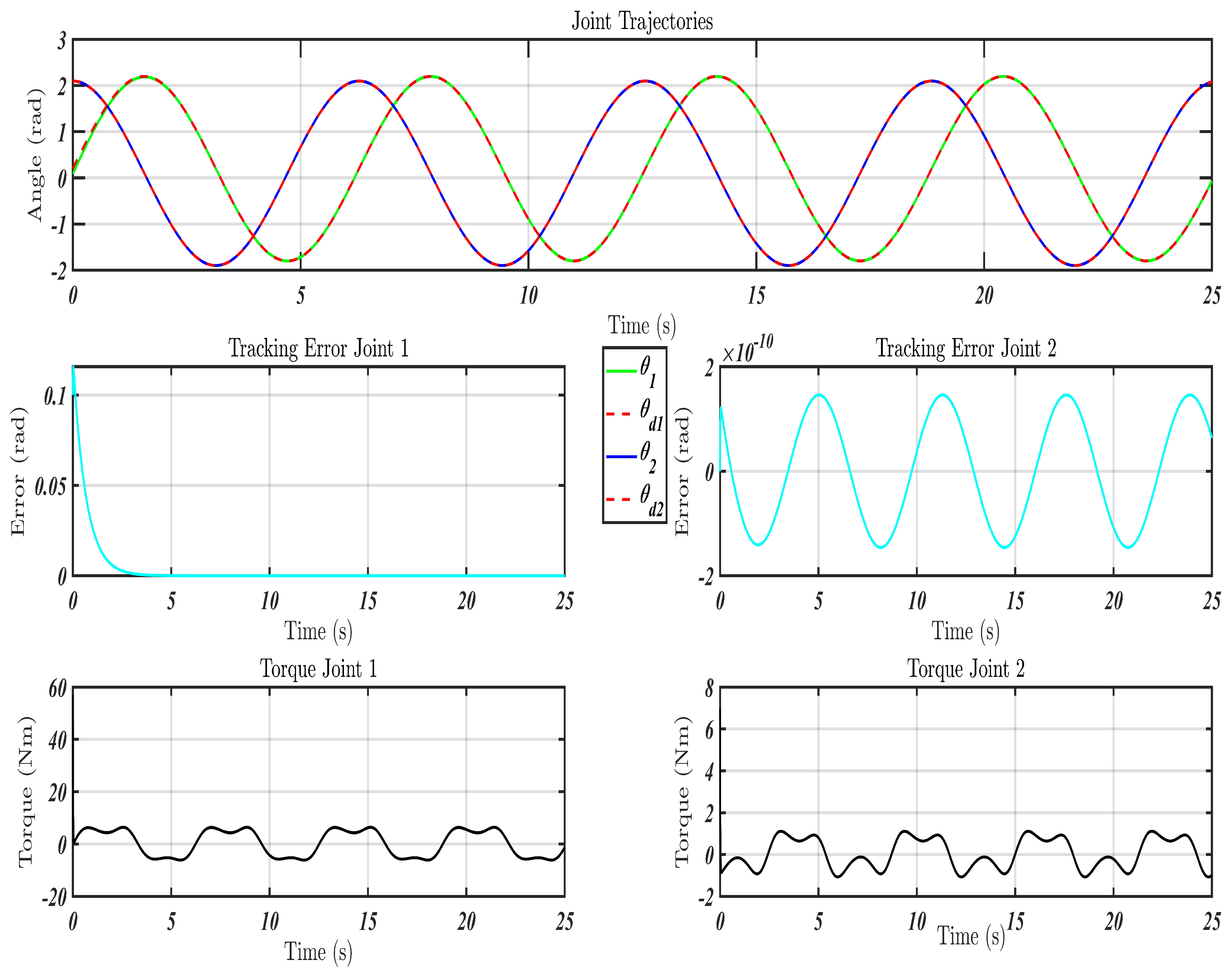
• Scenario 1: Nominal Conditions

In the first scenario, the conventional flatness-based control (FBC) method [30] under nominal conditions indicates that no external disturbances are present. The disturbance vector is set to zero: ${\zeta }_{\mathrm{dis}}=\mathbf{0}$.

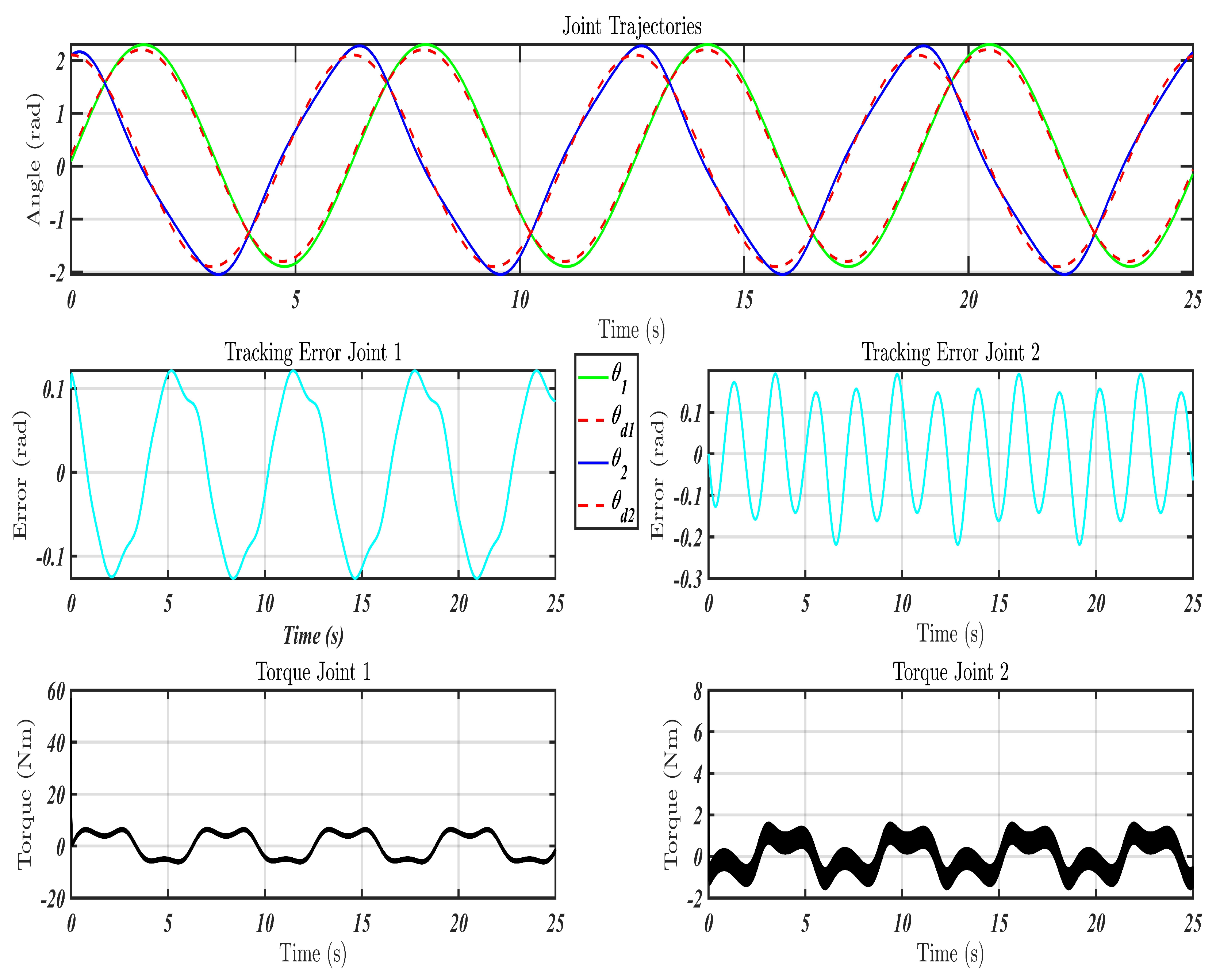
• Scenario 2: External Disturbance

In the second scenario, we apply the same control method, but this time the system experiences external disturbances that vary with time, represented by:

$$\begin{array}{c}\hfill {\zeta }_{\mathrm{dis}}=\left[\begin{array}{c}4sin\left(t\right)+0.5sin\left(200\pi t\right)\\ cos\left(3t\right)+0.5sin\left(200\pi t\right)\end{array}\right].\end{array}$$

(54)

• Scenario 3: Proposed Control Strategy

In the third scenario, the disturbance profile is established in Scenario 2 while implementing the proposed control strategy (refer to Equation (45)). This arrangement allows us to directly compare the performance of the proposed method with that of conventional approaches in the same conditions.

5.1. Trajectory and Control Parameters

The desired joint trajectory used in all simulations is defined as: ${\theta }_d\left(t\right)={[0.2+2sin\left(t\right),0.1+2cos\left(t\right)]}^T$. The control gains are established as follows for all scenarios:

$$\begin{array}{c}\hfill k_p=10I_{2\times 2},k_d=50I_{2\times 2},\end{array}$$

where $I_{2\times 2}$ represents the $2\times 2$ identity matrix. The parameters for the Kalman filter applied in the observer design are summarized below.

$$P=\left[\begin{array}{cccccccc}10& 0& 0& 0& 0& 0& 0& 0\\ 0& 10& 0& 0& 0& 0& 0& 0\\ 0& 0& 10& 0& 0& 0& 0& 0\\ 0& 0& 0& 10& 0& 0& 0& 0\\ 0& 0& 0& 0& 10& 0& 0& 0\\ 0& 0& 0& 0& 0& 10& 0& 0\\ 0& 0& 0& 0& 0& 0& 10& 0\\ 0& 0& 0& 0& 0& 0& 0& 10\end{array}\right];Q=\left[\begin{array}{cccccccc}10& 0& 0& 0& 0& 0& 0& 0\\ 0& 10& 0& 0& 0& 0& 0& 0\\ 0& 0& 10& 0& 0& 0& 0& 0\\ 0& 0& 0& 10& 0& 0& 0& 0\\ 0& 0& 0& 0& 10& 0& 0& 0\\ 0& 0& 0& 0& 0& 10& 0& 0\\ 0& 0& 0& 0& 0& 0& 10& 0\\ 0& 0& 0& 0& 0& 0& 0& 10\end{array}\right];$$

$$R=\left[\begin{array}{cc}10& 0\\ 0& 10\end{array}\right];$$

5.2. Performance Metrics

To comprehensively evaluate and compare the effectiveness of the control strategies, we employ various quantitative metrics, including the Mean Absolute Error (MAE) and the Standard Deviation of the Error (SDE). The metrics related to tracking errors are defined as follows:

$$\left\{\begin{array}{c}\mathrm{MAE}={\displaystyle \frac{1}{N}}\sum _{i=1}^N\parallel e\left(i\right)\parallel ,\hfill \\ \mathrm{SDE}=\sqrt{{\displaystyle \frac{1}{N}}{\sum }_{i=1}^N{\left(\parallel e\left(i\right)\parallel -\mathrm{MAE}\right)}^2},\hfill \end{array}\right.$$

(55)

where $e\left(i\right)$ denotes the tracking error at the i-th time step, while N refers to the total number of samples collected. Mean Absolute Error (MAE) measures the average size of the tracking error, whereas the Standard Deviation of the Error (SDE) assesses how much the errors vary. A low MAE reflects a high level of accuracy, and a low SDE signifies performance that is consistent and exhibits low variability. These two metrics are solely used in

Table 3. Performance comparison across different scenarios.

Performance	Scenario 1		Scenario 2		Scenario 3
	Joint 1	Joint 2	Joint 1	Joint 2	Joint 1	Joint 2
MAE (rad)	0.0032	0.0010	0.0789	0.1055	0.0561	0.0559
SDE (rad)	0.0136	0.0015	0.0345	0.0545	0.0254	0.0298

to compare the proposed controller against conventional methods [31].

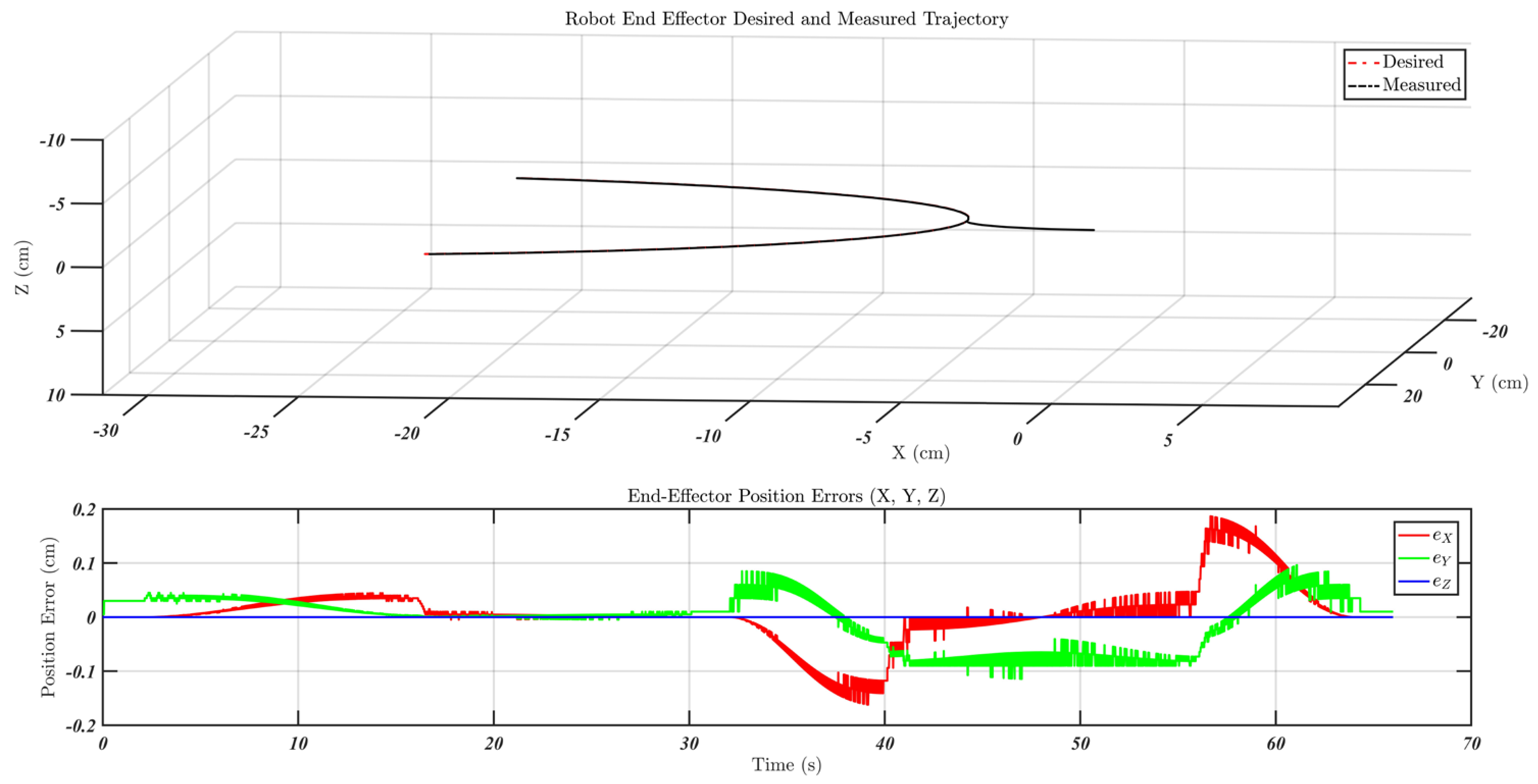
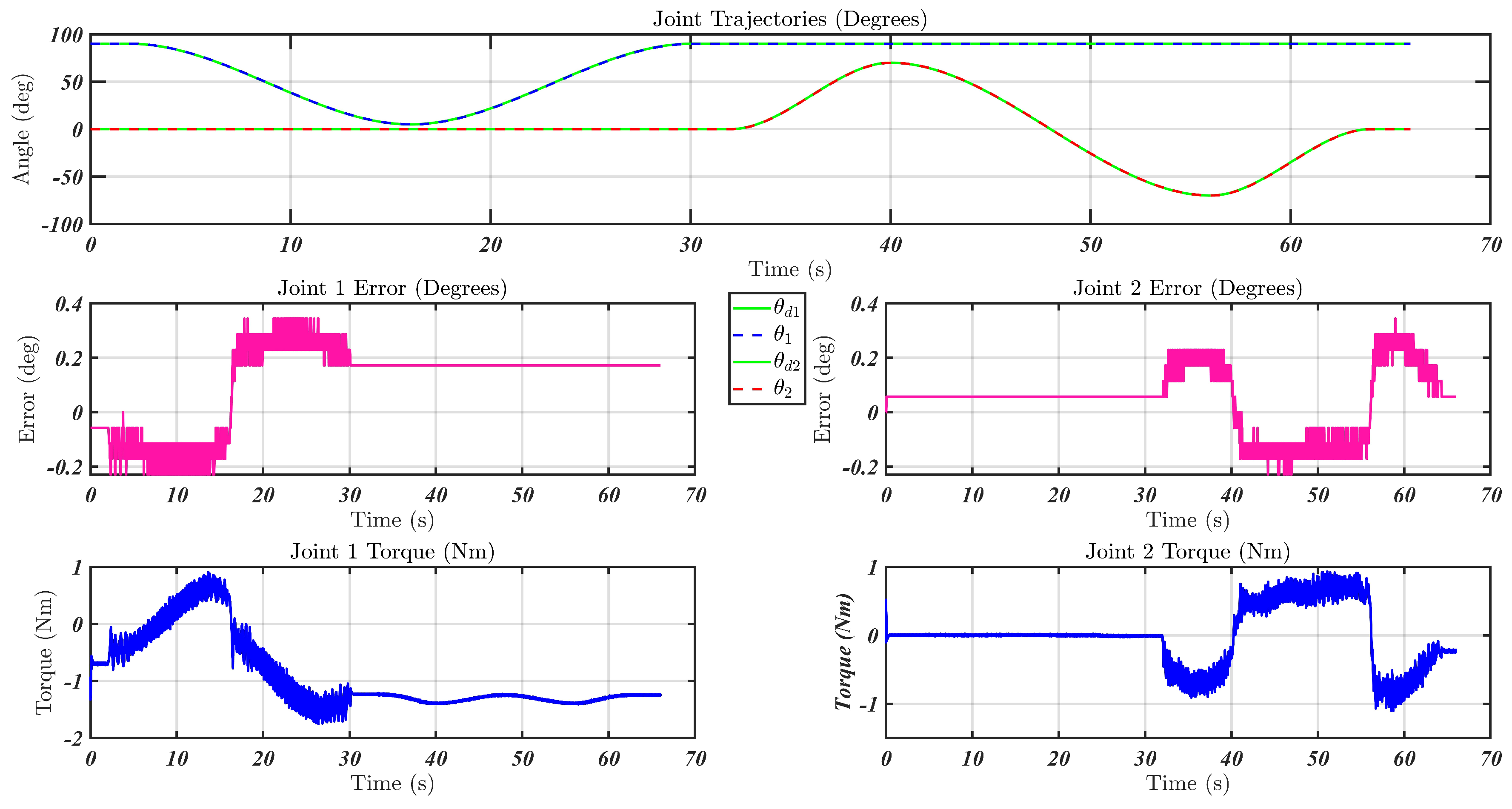
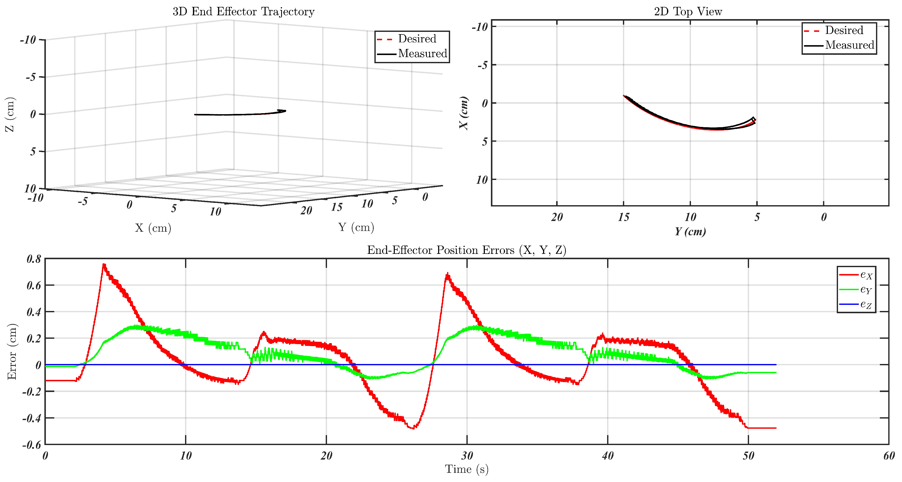
5.3. Simulation Results

Figure 6, Figure 7 and Figure 8 illustrate the trajectory tracking performance of different control strategies applied to the joint motion of the robotic system. Figure 6 presents the response obtained using a Flatness-Based Control (FBC) strategy under ideal conditions, where no external disturbances are introduced. The controller demonstrates satisfactory performance in tracking the desired joint trajectory, maintaining relatively smooth and accurate convergence. However, minor deviations observed at high-slope segments of the trajectory indicate a certain sensitivity of the control law to small model mismatches or measurement imperfections.

In contrast, Figure 7 evaluates the same flatness-based controller (FBC) under the influence of external disturbances (torque variations). As evident in the Figure 7, the control system exhibits increased tracking error, especially during dynamic transitions and at trajectory peaks. The presence of disturbances significantly deteriorates the controller’s performance, leading to overshoots, oscillations, and noticeable lag between the desired and actual trajectories. This result highlights a key limitation of standard FBC: its lack of inherent robustness against unmodeled dynamics.

To address these shortcomings, Figure 8 introduces the proposed improved control strategy, which integrates a Kalman filter into the flatness-based framework. The Kalman filter is employed to estimate the true system states and attenuate the effect of external disturbances. The resulting trajectory tracking performance is markedly improved compared to the previous cases. The proposed FBC-Kalman controller effectively suppresses noise-induced fluctuations and ensures smoother, more accurate tracking with minimal error. The system responds reliably even during rapid trajectory transitions, showcasing both stability and robustness.

The comparative analysis highlights the benefits of integrating the Kalman filter technique with the nonlinear control method. While the basic FBC performs well in ideal settings, it lacks robustness in disturbed environments. By incorporating a Kalman filter, the system’s resilience and tracking accuracy are greatly improved, making this integrated approach more applicable to real-world situations, especially in rehabilitation contexts where effectively managing disturbances is essential. This conclusion is further supported by the performance metrics detailed in Table 3.

6. Experimental Results

The iTbot rehabilitation robot system is built on a three-tier computing architecture. At the top level, a user interface (UI) on a personal computer enables control commands and real-time visualization of joint positions and force sensor data. The second level uses a National Instruments CompactRIO as a Real-Time (RT) controller, where LabVIEW RT applications handle trajectory planning, control algorithms, feedback processing, and data logging. At the lowest level, the system’s FPGA embedded within the CompactRIO executes fast-loop tasks every 50 $\mu$s, including PI motor current control and position measurement from motor hall-sensor signals. The robot’s joints are actuated by Maxon EC-45 Flat BLDC motors (30 W and 70 W models) paired with Harmonic Drive gearboxes (100:1 ratio), and powered by ZB12A servo amplifiers. The built-in hall sensors serve both for motor commutation and precise joint feedback.

Experimental Evaluation

The proposed control approach (45) was experimentally tested under two scenarios to assess its performance in practical conditions. In the first scenario, a simple physiotherapy task was conducted. The subject’s hand was attached to the end-effector of the exoskeleton robot and guided through a predefined trajectory. In this case, the external disturbance originated from the subject’s natural interaction with the robot during motion execution. The second scenario involved a repetitive task, designed to evaluate the controller’s robustness under continuous human–robot contact and dynamic parameter variations introduced by repeated movements. This setup mimics realistic rehabilitation activities where disturbances and nonlinearities may arise over time. The controller gains used in both experiments were: $k_p=18I_{2\times 2},k_d=75I_{2\times 2}$. The Kalman filter parameters remained the same as specified in the previous section. Experimental results are presented in both joint space and Cartesian space, utilizing the Jacobian matrix to perform coordinate transformations between these domains.

• Scenario 1: simple motion

In Scenario 1, which involves a guided physiotherapy task with moderate external interference from human interaction, the proposed control scheme demonstrates strong trajectory tracking capabilities in Cartesian space (Figure 9). The desired and actual end-effector paths show a close match, with minimal deviation along all three axes. The position error plots confirm this observation, maintaining sub-millimeter deviations in most instances and not exceeding $\pm 0.2$ cm in any axis. This high level of precision highlights the controller’s ability to reject mild disturbances and ensure smooth motion execution.

Joint space analysis (Figure 10) reinforces this performance. The actual joint angles accurately follow the reference trajectories for both joints, with maximum joint errors staying below $\pm 0.4$ degrees. The smoothness of the joint torque signals, particularly in the first joint, suggests effective damping behavior and a lack of abrupt corrective actions. This behavior indicates good compliance with minimal overshooting, which is essential for safe human–robot interaction during rehabilitation exercises.

• Scenario 2: repetitive motion

In Scenario 2, involving repetitive tasks and dynamic variations due to continued human contact, the control system maintains stable performance, albeit under more challenging conditions (Figure 11 and Figure 12). Although Cartesian tracking remains precise, noticeable deviations, particularly along the X and Y axes, where peak position errors can increase by up to $\pm 0.8$ cm. These errors reflect the increased difficulty of maintaining precision under time-varying disturbances and unmodeled dynamics. Nonetheless, the system recovers promptly from disturbances, suggesting robust adaptive behavior.

Joint space metrics in Figure 12 reveal higher joint angle errors compared to Scenario 1, with values reaching up to $\pm 2$ degrees in Joint 1. The torque profiles exhibit more aggressive corrective actions, indicative of the controller’s responsiveness to persistent disturbances. Despite these challenges, trajectory following remains stable and smooth, with no signs of instability or oscillations, which emphasizes the effectiveness of the proposed control law even under non-ideal conditions.

7. Conclusions

This study addresses the challenge of implementing robust, adaptive, and safe control mechanisms in end-effector-based rehabilitation robots, focusing on the iTbot platform for upper-limb therapy. Traditional controllers often struggle with dynamic uncertainties and the interaction forces that arise during human–robot collaboration. To overcome these issues, we propose a flatness-based control framework augmented with a derivative-free Kalman filter (DFK) for real-time state estimation and disturbance rejection. By transforming the nonlinear dynamics into a 0-flat canonical form, the proposed approach streamlines trajectory tracking while preserving computational efficiency. Extensive simulations and hardware experiments show that the proposed controller greatly improves tracking accuracy and robustness relative to a conventional flatness-based controller, both in disturbance-free conditions and under deliberately applied external disturbances. These enhancements yield smoother, more compliant motion—essential for safe and effective rehabilitation—and underscore the method’s potential for clinical and home use, where accessible, high-quality therapy is crucial. Nonetheless, the current study is limited to a two-degrees-of-freedom system and predefined disturbance profiles, which do not fully capture the variability of real patient interactions. Future work will extend the framework to multi-DoF manipulators, integrate human-intent recognition, and validate its effectiveness through clinical trials involving diverse patient populations.

References

1. Yu, S.; Huang, T.H.; Yang, X.; Jiao, C.; Yang, J.; Chen, Y.; Yi, J.; Su, H. Quasi-Direct Drive Actuation for a Lightweight Hip Exoskeleton with High Backdrivability and High Bandwidth. IEEE/ASME Trans. Mechatron. 2020, 25, 1794–1802. [Google Scholar] [CrossRef] [PubMed]
2. Teng, L.; Gull, M.A.; Bai, S. PD Based Fuzzy Sliding Mode Control of A Wheelchair Exoskeleton Robot. IEEE/ASME Trans. Mechatron. 2020, 25, 2546–2555. [Google Scholar] [CrossRef]
3. Balasubramanian, S.; Wei, R.; Perez, M.; Shepard, B.; Koeneman, E.; Koeneman, J.; He, J. RUPERT: An exoskeleton robot for assisting rehabilitation of arm functions. In Proceedings of the 2008 Virtual Rehabilitation, Vancouver, BC, Canada, 25–27 August 2008; pp. 163–167. [Google Scholar]
4. Xiao, F.; Gao, Y.; Wang, Y.; Zhu, Y.; Zhao, J. Design of a wearable cable-driven upper limb exoskeleton based on epicyclic gear trains structure. Technol. Health Care 2017, 25, 3–11. [Google Scholar] [CrossRef] [PubMed]
5. Khan, M.M.R.; Ahmed, T.; Pallares, J.R.H.; Islam, M.R.; Brahmi, B.; Rahman, M.H. Development of A Desktop-mounted Rehabilitation Robot For Upper Extremities. In Proceedings of the International Conference on Industrial Mechanical Engineering and Operations Management, Dhaka, Bangladesh, 26–27 December 2021. [Google Scholar]
6. Cao, W.; Chen, C.; Hu, H.; Fang, K.; Wu, X. Effect of hip assistance modes on metabolic cost of walking with a soft exoskeleton. IEEE Trans. Autom. Sci. Eng. 2020, 18, 426–436. [Google Scholar] [CrossRef]
7. Loureiro, R.C.; Harwin, W.S.; Nagai, K.; Johnson, M. Advances in upper limb stroke rehabilitation: A technology push. Med. Biol. Eng. Comput. 2011, 49, 1103–1118. [Google Scholar] [CrossRef]
8. Nef, T.; Guidali, M.; Riener, R. ARMin III–arm therapy exoskeleton with an ergonomic shoulder actuation. Appl. Bionics Biomech. 2009, 6, 127–142. [Google Scholar] [CrossRef]
9. Kim, B.; Deshpande, A.D. An upper-body rehabilitation exoskeleton Harmony with an anatomical shoulder mechanism: Design, modeling, control, and performance evaluation. Int. J. Robot. Res. 2017, 36, 414–435. [Google Scholar] [CrossRef]
10. Liu, L.; Shi, Y.Y.; Xie, L. A novel multi-dof exoskeleton robot for upper limb rehabilitation. J. Mech. Med. Biol. 2016, 16, 1640023. [Google Scholar] [CrossRef]
11. Pignolo, L.; Dolce, G.; Basta, G.; Lucca, L.; Serra, S.; Sannita, W. Upper limb rehabilitation after stroke: ARAMIS a “robo-mechatronic” innovative approach and prototype. In Proceedings of the 2012 4th IEEE RAS-EMBS International Conference on Biomedical Robotics and Biomechatronics (BioRob), Rome, Italy, 24–27 June 2012; pp. 1410–1414. [Google Scholar]
12. Bououden, S.; Boutat, D.; Zheng, G.; Barbot, J.P.; Kratz, F. A triangular canonical form for a class of 0-flat nonlinear systems. Int. J. Control 2011, 84, 261–269. [Google Scholar] [CrossRef]
13. Zhang, L.; Guo, S.; Sun, Q. Development and assist-as-needed control of an end-effector upper limb rehabilitation robot. Appl. Sci. 2020, 10, 6684. [Google Scholar] [CrossRef]
14. Brahmi, B.; Saad, M.; Rahman, M.H.; Ochoa-Luna, C. Cartesian trajectory tracking of a 7-DOF exoskeleton robot based on human inverse kinematics. IEEE Trans. Syst. Man Cybern. Syst. 2017, 49, 600–611. [Google Scholar] [CrossRef]
15. Chen, W.; Ge, S.S.; Wu, J.; Gong, M. Globally stable adaptive backstepping neural network control for uncertain strict-feedback systems with tracking accuracy known a priori. IEEE Trans. Neural Netw. Learn. Syst. 2015, 26, 1842–1854. [Google Scholar] [CrossRef] [PubMed]
16. Yoo, B.K.; Ham, W.C. Adaptive control of robot manipulator using fuzzy compensator. IEEE Trans. Fuzzy Syst. 2000, 8, 186–199. [Google Scholar]
17. Craig, J.J. Introduction to Robotics: Mechanics and Control (Pearson Prentice Hall Upper Saddle River, 2005). Available online: https://marsuniversity.github.io/ece387/Introduction-to-Robotics-Craig.pdf (accessed on 25 May 2025).
18. Siciliano, B.; Sciavicco, L.; Villani, L.; Oriolo, G. Kinematics; Springer: Berlin/Heidelberg, Germany, 2009. [Google Scholar]
19. Ferrer, S.; Ochoa-Luna, C.; Rahman, M.; Saad, M.; Archambault, P. HELIOS: The Human Machine Interface forMARSERobot. In Proceedings of the 6th International Conference on Human System Interaction (HSI), Sopot, Poland, 6–8 June 2013; pp. 117–122. [Google Scholar]
20. Luna, C.O.; Rahman, M.H.; Saad, M.; Archambault, P.; Zhu, W.-H. Virtual decomposition control of an exoskeleton robot arm. Robotica 2016, 34, 1587–1609. [Google Scholar] [CrossRef]
21. Rahman, M.H.; Kittel-Ouimet, T.; Saad, M.; Kenné, J.P.; Archambault, P.S. Dynamic modeling and evaluation of a robotic exoskeleton for upper-limb rehabilitation. Int. J. Inform. Acquis. 2011, 8, 83–102. [Google Scholar] [CrossRef]
22. Chen, P.; Chen, C.-W.; Chiang, W.-L. GA-based modified adaptive fuzzy sliding mode controller for nonlinear systems. Expert Syst. Appl. 2009, 36, 5872–5879. [Google Scholar] [CrossRef]
23. Brahmi, B.; Saad, M.; Luna, C.O.; Archambault, P.S.; Rahman, M.H. Passive and active rehabilitation control of human upper-limb exoskeleton robot with dynamic uncertainties. Robotica 2018, 36, 1757–1779. [Google Scholar] [CrossRef]
24. Rigatos, G.G. Extended Kalman and particle Filtering for sensor fusion in motion control of mobile robots. Math. Comput. Simul. 2010, 81, 590–607. [Google Scholar] [CrossRef]
25. Rigatos, G.; Zhang, Q. Fuzzy Model Validation Using the Local Statistical Approach; IRISA No 1417; Publication Interne: Rennes, France, 2001. [Google Scholar]
26. Fliess, M.; Levine, J.; Martin, P.; Rouchon, P. Flatness and Defect of Non-Linear Systems: Introductory Theory and Examples. Int. J. Control 1995, 61, 1327–1361. [Google Scholar] [CrossRef]
27. Fliess, M.; Levine, J.; Martin, P.; Rouchon, P. On differentially flat nonlinear systems. In Proceedings of the 2nd IFAC-Symposium on Nonlinear Control Systems, Bordeaux, France, 24–26 June 1992; pp. 159–163. [Google Scholar]
28. Murray, M.P.M.; Rouchon, P. Flat systems. In Advances in the Control of Nonlinear Systems, Plenary Lectures and Mini-Courses, Proceedings of the 4th European Control Conference ECC 97, Brussels Belgium, 1–4 July 1997; Gevers, M., Bastin, G., Eds.; Springer: London, UK, 1997; pp. 211–264. [Google Scholar]
29. Ramirez, H.S.; Agrawal, S.K. Differentially Flat Systems; Marcel Dekker: New York, NY, USA, 2004. [Google Scholar]
30. Brahmi, B.; Ahmed, T.; El Bojairami, I.; Swapnil, A.A.Z.; Assad-Uz-Zaman, M.; Schultz, K.; McGonigle, E.; Rahman, M.H. Flatness based control of a novel smart exoskeleton robot. IEEE/ASME Trans. Mechatronics 2021, 27, 974–984. [Google Scholar] [CrossRef]
31. Khan, M.M.R.; Swapnil, A.A.Z.; Ahmed, T.; Rahman, M.M.; Islam, M.R.; Brahmi, B.; Fareh, R.; Rahman, M.H. Development of an end-effector type therapeutic robot with sliding mode control for upper-limb rehabilitation. Robotics 2022, 11, 98. [Google Scholar] [CrossRef]
32. Chen, Y.; Fan, J.; Zhu, Y.; Zhao, J.; Cai, H. A passively safe cable driven upper limb rehabilitation exoskeleton. Technol. Health Care 2015, 23, S197–S202. [Google Scholar] [CrossRef] [PubMed]
33. Luh, J.Y.; Walker, M.W.; Paul, R.P. On-line computational scheme for mechanical manipulators. J. Dyn. Syst. Meas. Control 1980, 102, 69–76. [Google Scholar] [CrossRef]
34. Pereira da Silva, P.S. Flatness of nonlinear control systems: A Cartan-Kähler approach. In Proceedings of the Mathematical Theory of Networks et Systems, MTNS 2000, Perpignan, France, 19–23 June 2000; pp. 1–10. [Google Scholar]
35. Isidori, A. Nonlinear Control Systems, 3rd ed.; Springer: Berlin/Heidelberg, Germany, 1995. [Google Scholar]
36. Rigatos, G.G.; Tzafestas, S.G. Extended Kalman filtering for fuzzy modelling and multisensor fusion. Math. Comput. Model. Dyn. Syst. 2007, 13, 251–266. [Google Scholar] [CrossRef]
37. Rigatos, G.; Siano, P.; Zervos, N. Derivative-free nonlinear Kalman filtering for PMSG sensorless control. In Mechatronics Engineering: Research Development and Education; Habib, M., Ed.; Wiley: Hoboken, NJ, USA, 2012. [Google Scholar]
38. Rigatos, G.; Siano, P. A derivative-free extended information filtering approach for sensorless control of nonlinear systems. In Proceedings of the MASCOT 2010, IMACS Workshop on Scientific Computation; Italian Institute for Calculus Applications: Gran Canaria, Spain, 2010. [Google Scholar]
39. Chen, W.H.; Ballance, D.J.; Gawthrop, P.J.; Reilly, J.O. A nonlinear disturbance observer for robotic manipulators. IEEE Trans. Industr. Electron. 2000, 47, 932–938. [Google Scholar] [CrossRef]
40. Cortesao, R. On Kalman active observers. J. Intell. Robot. Syst. 2006, 48, 131–155. [Google Scholar] [CrossRef]
41. Slotine, J.J.E.; Li, W. Applied Nonlinear Control; Prentia Hall: Englewood Cliffs, NJ, USA, 1991. [Google Scholar]
Figure 1. Mechanical architecture of the iTbot platform illustrating the main structural and actuation components involved in the mechanical design [31].
Actuators 14 00341 g001
Figure 4. iTbot nomenclature for dynamic modeling, including contact force at the end-effector.
Actuators 14 00341 g004
Figure 5. Global schematic of proposed control for iTbot robot.
Actuators 14 00341 g005
Figure 6. Joint trajectory tracking using flatness-based control [31].
Actuators 14 00341 g006
Figure 7. Joint trajectory tracking using flatness-based control under external disturbances.
Actuators 14 00341 g007
Figure 8. Joint trajectory tracking using the proposed controller (45).
Actuators 14 00341 g008
Figure 9. Cartesian trajectory tracking and position error in a simple physiotherapy task (Scenario 1).
Actuators 14 00341 g009
Figure 10. Joint space tracking, error, and torque response in a simple physiotherapy task (Scenario 1).
Actuators 14 00341 g010
Figure 11. Cartesian trajectory tracking and position error in a repetitive task (Scenario 2).
Actuators 14 00341 g011
Figure 12. Joint space tracking, error, and torque response in a repetitive task (Scenario 2).
Actuators 14 00341 g012