Article

Distributed Adaptive Angle Rigidity-Based Formation Control of Near-Space Vehicles with Input Constraints

1
College of Information Engineering, Yangzhou University, Yangzhou 225127, China
2
College of Education, Yancheng Teachers University, Yancheng 224007, China
*
Author to whom correspondence should be addressed.
Actuators 2025, 14(7), 339; https://doi.org/10.3390/act14070339
Submission received: 27 May 2025 / Revised: 6 July 2025 / Accepted: 7 July 2025 / Published: 8 July 2025
(This article belongs to the Section Aerospace Actuators)

Abstract

This paper presents a distributed adaptive formation control strategy for a multiple near-space vehicles (NSVs) system operating under unknown input constraints and external disturbances. In challenging near-space environments, the control system must address not only model uncertainties and parameter variations but also accommodate the input limitations of actuators. To address these challenges, we design an adaptive distributed formation control strategy for vehicle formation that relies exclusively on relative attitude information. This approach is grounded in the principles of angle rigidity formation theory, which has not previously been applied in the near-space vehicle domain. The aim of the adaptive formation control strategy is to maintain the desired formation shape for the near-space vehicles (NSVs) system with external disturbances, actuator dead zones, and saturation. In addition, neural networks are employed to approximate the inherent nonlinear uncertainties within the NSV models. An adaptive estimation technique is concurrently included to address parameter variations and to alleviate the impact of external disturbances, actuator dead zones, and saturation effects. Finally, a Lyapunov-based analysis is used to rigorously demonstrate the stability of the NSV formation system. The simulation results validate the effectiveness and robustness of the proposed control strategy in uncertain environments.

1. Introduction

In the expansive and distinctive realm of near space, which refers specifically to the region spanning from 20 to 100 km above ground level, the demarcation between conventional aviation and outer-space aviation becomes increasingly indistinct [1,2,3,4,5,6]. Technology for the spatial formation of near-space vehicles (NSVs) is gaining significant recognition, and its innovation and practicality make it a prominent research focus [7,8]. Increasing the number of spacecraft enhances cooperative sensing and mid-course guidance capabilities, reducing the demands on individual spacecraft and lowering mission costs [9,10,11]. Furthermore, it improves target tracking and interception in missions that involve multiple interceptors. Coordinated flight formations provide cost-effective solutions for complex missions [12,13,14,15,16].
As noted in [17,18,19], an NSV formation system must address the complexities of subsonic, transonic, and supersonic flight phases. Throughout this process, it is imperative to effectively handle the significant aerodynamic environment changes and highly nonlinear geothermal effects at high temperatures. In addition, the control challenges arising from model parameter uncertainties and unpredictable external disturbances generated by the environment need to be overcome [20,21,22]. To solve these problems, existing studies address uncertainties using methods like sliding mode disturbance observers [23], support vector regression for nonlinearities [24], and fault-tolerant control technologies [25]. Neural networks (NNs) have also been used to approximate model uncertainties and mitigate disturbances [6,26], effectively addressing some issues of uncertainty. Beyond the challenges of model uncertainties and parameter variations in the unique near-space environment, the control system must also address the limitations imposed by the input constraints of the actuator. Near-space formation systems face efficiency challenges from “dead zones” [27,28]. Adaptive NN control [29] and filtering algorithms [30] have been proposed to mitigate this. Additionally, actuator saturation during the entry phases limits the NSV performance, with attitude angles often coming close to safety limits [31,32] and torques being constrained by bounded surface angles [33]. Nevertheless, these studies address only some parts of the problem and focus solely on single NSVs, and they overlook the complex coupling and coordination challenges that are inherent to formations. These simultaneous challenges require integrated solutions to enhance the stability and performance of NSV formation.
In recent years, the formation tracking of hypersonic vehicles was achieved by Zhang et al. [34] through fixed-time stability-based control. To minimize communication while maintaining tracking performance, Lv et al. [8] designed a dynamic event-triggered protocol that used output feedback. In addition, Zuo et al. [35] introduced a learning-based containment strategy with event-triggered communication to ensure that HFVs remained within the leader’s convex hull without requiring frequent updates to the NN. Furthermore, a globally distributed protocol that used fixed time for collision-free formation tracking with rapid responses was developed by Wu et al. [7]. Note that the majority of the aforementioned studies primarily utilize consensus strategies, relative position data, or complete system information. The control problem relating to attitude coordination between spacecraft flying in formation was proposed in [36,37], where only a subset of members have access to the common reference attitude. A distributed predefined time control was studied in [38], where only some spacecraft have access to the reference attitude and angular velocity. Zhuang et al. [39] investigated the fixed-time stability of attitude coordination control for spacecraft formation flying under external disturbances. Nonetheless, the aforementioned studies do not adequately address problems related to the stability of the formation, model uncertainties, parameter variations, and actuator input limitations. As a result, ensuring stable formation control for multiple NSVs in the presence of input constraints and external disturbances continues to pose a considerable challenge.
Inspired by angle rigidity formation theory, this study addresses the control problem related to rigid angle formation for NSVs in the presence of modeling inaccuracies, external disturbances, and input constraints. The primary contributions of this work are summarized as follows:
  • Unlike previous studies [7,8,18] that have primarily relied on relative position data for formation control, this study presents a novel distributed formation-control strategy for multiple NSVs that relies exclusively on relative attitude angles. By pioneering the application of angle rigidity theory, the proposed method significantly improves the formation stability, robustness, and adaptability.
  • In contrast to prior research [34,37,38,39], which has addressed actuator dead zones, saturation, external disturbances, and model uncertainties as isolated problems, this study addresses these interconnected challenges concurrently within the context of multiple NSV formation systems. Specifically, an NN-based adaptive control methodology is proposed that ensures stable and robust system performance in the presence of these combined conditions.
The remainder of this paper is organized as follows. Section 2 presents the mathematical modeling of near-space vehicles (NSVs) and reformulates the system dynamics to include dead-zone and saturation effects. Section 3 introduces the angle rigidity-based formation framework and details the distributed control law along with adaptive estimation strategies. Section 4 provides a rigorous stability analysis using Lyapunov-based techniques to prove the convergence of the formation system under external disturbances and input constraints. Section 5 validates the proposed method through simulation results for triangular, hexagonal, and octagonal NSV formations. Finally, Section 6 concludes the paper and outlines potential directions for future research.

2. Problem Statement

The dynamic equations of a NSV (near-space vehicle) attitude system are expressed as follows [23,40]:
Ω ˙ = f s + g 1 ω ,
ω ˙ = K 1 Ω ( ω ) K ω + K 1 g 2 δ c ,
where Ω = [ α , β , μ ] T represents the attitude angles, including the angle of attack ( α ), sideslip angle ( β ), and banking angle ( μ ). ω = [ p , q , r ] T denotes the attitude angular rates, comprising the roll rate (p), pitch rate (q), and yaw rate (r). The control surface deflections of the elevator, aileron, and rudder are represented by δ c = [ δ e , δ a , δ r ] T , respectively. K R 3 × 3 is the inertia matrix, whose elements are nonlinear functions of the NSV mass.
f s = f α f β f μ , g 1 = tan β cos α 1 tan β sin α sin α 0 cos α sec β cos α 0 sec β sin α ,
Ω ( ω ) = 0 r q r 0 p q p 0 , g 2 = g α , δ e g α , δ a g α , δ r g β , δ e g β , δ a g β , δ r g μ , δ e g μ , δ a g μ , δ r .
Here, f s and g 2 depend on Ω and various system parameters, including the vehicle’s mass, flight velocity, dynamic pressure, and aerodynamic coefficients, among other parameters. The components f α , f β , and f μ represent the nonlinear dynamic terms corresponding to the angle of attack, sideslip angle, and bank angle, respectively, and are functions of the NSV’s mass, flight velocity, dynamic pressure, and aerodynamic coefficient. The elements g α , δ e , g α , δ a , g α , δ r , etc., in g 2 denote the control effectiveness coefficients, describing the influence of control surface deflections ( δ e , δ a , δ r ) on the attitude angles ( α , β , μ ).
Assumption 1.
The bank-to-turn maneuver strategy is adopted to maintain a near-zero sideslip angle during flight, avoiding the singularity at β = ± 90 ° [41].
Due to the singularity in (1) when β = ± 90 ° , Assumption 1 ensures the model’s validity. This strategy aligns with hypersonic vehicle control practices where near-zero sideslip angles enhance stability and controllability.
Equations (1) and (2) describe slow-loop and fast-loop attitude systems. Considering the uncertainties and disturbances that act on an NSV, these systems can be expressed as affine nonlinear equations [31,40]:
Ω ˙ ( t ) = h s ( Ω ( t ) ) + g s ( Ω ( t ) ) ω ( t ) + d s ( t ) y s ( t ) = Ω ( t ) ,
ω ˙ ( t ) = h f ( ω ( t ) ) + g f ( ω ( t ) ) M C ( t ) + d f ( t ) y f ( t ) = ω ( t ) ,
where x s = Ω ( t ) , r s = ω ( t ) , x f = ω ( t ) , and r f = M C = g 2 δ c represent the slow-loop state, slow-loop input, fast-loop state, and fast-loop input, respectively. h s ( Ω ) = f s , g s ( Ω ) = g 1 , h f ( ω ) = K 1 Ω ( ω ) K ω , and g f ( ω ) = K 1 are the system matrices. Note that d s ( t ) and d f ( t ) represent the external disturbances. Here, M C ( t ) denotes the control torque generated by deflection of the elevator, aileron, and rudder surfaces.
Remark 1.
A change in the control surface deflection δ c directly affects the moment M C applied to the NSV, whereas the effects on p ˙ , q ˙ , r ˙ are significant. However, the effects on α ˙ , β ˙ , μ ˙ are relatively minor. Therefore, when the time-scale separation principle and singular perturbation method are used, Ω and ω are considered as the system’s slow- and fast-loop states, respectively. Accordingly, the NSV attitude control can be divided into fast- and slow-loop control structures. This standard affine nonlinear system of Equations (3) and (4) can be used as the basis for designing controllers for the slow loop and fast loop.

2.1. System Model

To illustrate the design process for an attitude controller within a formation control system, we analyze a general affine nonlinear MIMO system [23,42]. This system encompasses multiple constraints, including system modeling functions, external time-varying disturbances, and control input constraints.
x ˙ i ( t ) = f i ( x i ) + g i ( x i ) Sat ( φ i ( u i ) ) + d i ( t ) y i ( t ) = x i ( t ) , i = 1 , 2 , , n .
Let x i ( t ) R k denote the attitude angle of the i-th NSV, where i = 1 , 2 , , n corresponds to an individual vehicle in the system. The function Sat ( φ i ( u i ) ) R k represents the output from the dead-zone saturation model, which is driven by the control input u i R k . Additionally, f i ( x i ) R k × k defines a continuously smooth function that captures the nonlinear dynamics that are unique to each NSV, and the control gain matrix g i ( x i ) R k × k includes known, continuously smooth functions. The external disturbances that impact the system are modeled as d i ( t ) R k .
In NSV systems, dead zones introduce a range within which small control inputs yield no corresponding output, thereby reducing system responsiveness and control efficiency. Similarly, saturation occurs when the control inputs exceed the actuator limits, and this results in diminished control precision and potential instability. These problems highlight the need for advanced control strategies to maintain stable and reliable operation. The function φ i ( u i ) R k represents the input to the saturation model for the i-th NSV, mapping the control input u i to the actuator response before saturation effects are applied. The dead-zone saturation model, which is defined by the control input u i and the output Sat ( φ i ( u i ) ) R k , is expressed as follows:
Sat ( φ i ( u i ) ) = Sat ( φ i 1 ( u i 1 ) ) Sat ( φ i 2 ( u i 2 ) ) Sat ( φ i k ( u i k ) ) ,
Sat ( φ i l ( u i l ) ) is defined as
Sat ( φ i ( u i l ) ) = u H i l , u i l > u H i l α + i l + u + i l α + i l ( u i l u + i l ) , u H i l α + i l + u + i l > u i l > u + i l 0 , u i l < u i l < u + i l α i l ( u i l + u i l ) , u L i l α i l u i l < u i l < u i l u L i l , u i l < u L i l α i l u i l .
where l = 1 , 2 , n . As shown in Figure 1, the actuator dynamics are characterized by dead zones and saturation.
The control signal u i l is constrained by known bounds, where u L i l and u H i l represent the lower and upper limits, respectively. Additionally, u + i l and u i l signify the unknown threshold values of the dead-zone activation points, associated with α + i l and α i l . These thresholds are assumed to be bounded, nonzero constants.
To design the stabilized formation-control strategy with no loss of generality, we make the following assumption.
Assumption 2.
The external disturbance d i ( t ) R k is assumed to be bounded such that d i ( t ) D i , where D i is an unknown positive constant.
Assumption 3.
The difference between saturation-limited control and actual control Δ u i = Sat ( φ i ( u i ) ) φ i ( u i ) is conjectured to be within Δ u i Δ u i M , where Δ u i M is an unknown positive constant boundary.

2.2. Problem Transformation

Since the NSV formation system (5) exhibits modeling inaccuracies, Radial Basis Function Neural Networks (RBFNNs) are widely used for approximating unknown nonlinear functions over compact sets. Consider an unknown nonlinear function f i ( x ) defined on a compact set Ω i R m mapping to R . This function can be approximated with arbitrary accuracy using an RBFNN [43,44], which is represented as follows:
f i ( x i ) = ϕ i ( χ i ) θ i + δ i .
Here, x i = χ i , 1 T R m + 1 denotes the input vector, and θ i represents the optimal weight vector in R k , where k is the number of neurons or nodes in the network. Increasing the number of nodes generally improves the accuracy of the approximation. The weight vector θ i is determined by solving the following optimization problem:
θ i = arg min θ i ^ R k sup x i Ω x i | f i ( x i ) ϕ i ( χ i ) θ i ^ | .
In this context, θ i ^ is an estimate of the optimal weight vector θ i . The vector ϕ i ( χ i ) = [ Φ i 1 ( χ i ) , Φ i 2 ( χ i ) , , Φ i k ( χ i ) ] T denotes the radial basis function (RBF) vector, where each function Φ i l ( χ i ) is typically selected as a Gaussian function:
Φ i l ( χ i ) = exp χ i μ i l 2 ( σ i l ) 2 , l = 1 , , k .
The parameters μ i l R m and σ i l R are the center and spread of the RBF, respectively. The term ϵ i represents the approximation error, which is bounded over Ω i , such that | δ i | δ i ¯ , where δ i ¯ is an unknown constant.
According to the above conclusion, the function f i ( x i ) can be approximated by an RBFNN as follows:
f i ( x i ) = ϕ i ( χ i ) θ i + δ i .
By substituting Equation (10) into the system Equation (5), we obtain
x ˙ i ( t ) = ϕ i ( χ i ) θ i + g i ( x i ) Sat ( φ i ( u i ) ) + δ i + d i ( t ) y i ( t ) = x i ( t ) , i = 1 , 2 , , n .
This reformulation is crucial for understanding how the system evolves over time under the influence of control inputs and disturbances, providing a solid foundation for further analysis and controller design.

3. Graph Theoretical and Angle Rigidity

In this study, the problem of angle rigidity formation is considered. To achieve a stable formation, both the communication relations and the theory of angle rigidity are introduced.
The communication relations within a formation are represented by an undirected topology graph G = ( V , E ) in which V is the set of nodes and E is the set of edges. Vectors x i j = x i x j represent the relative attitude angle between NSV i and j, where x i j denotes the target relative attitude. Additionally, the directed form of the graph is represented by G . The edges in the graph G are labeled from 1 to m, where m denotes the number of edges. The incidence matrix H ( G ) is obtained by considering all edges E 1 , E 2 , , E m and is defined as follows:
H = H ( G ) = ( h i j ) R m × n .
Here, H is a matrix consisting of 0 , 1 , and 1 , and it is the same as that defined in [45]. We denote the vectors that represent the attitude angle of the i-th NSV as x = [ x 1 T , x 2 T , , x n T ] T . According to the definition of an incidence matrix, we obtain
e = H I n x = H ¯ x ,
where ⊗ represents the Kronecker product, and I n R n n denotes the identity matrix.
Angle rigidity is crucial to maintaining the structural integrity of a framework, particularly in three-dimensional spaces. This rigidity maintains the angle relationships between vertices in the event of small disturbances, thereby preserving their geometric arrangement. A framework is said to be angularly rigid if, for any equivalent framework A whose position vectors are perturbed, the corresponding angles remain congruent [46]. Minimal angle rigidity is defined as the state in which the removal of any single angle constraint causes a loss of rigidity, and the condition | A | = 3 | V | 7 determines the minimal number of angle constraints required to maintain rigidity [47].

4. Controller Design

4.1. Control Goal

The aim of this study is to design the necessary formation control laws u i . For any initial conditions x i ( 0 ) R n × n , i = 1 , 2 , , n , the NSV formation system achieves a globally and asymptotically stable formation. That is, the entire system converges to the set M, which is defined as follows:
M = x i j x i j = x i j , i = 1 , 2 , , n , j N i ,
where x i j represents the target relative attitude of NSV i with respect to its neighbor j, and N i is the set of neighbors of NSV i in the communication topology.

4.2. Controllers

We define the potential energy function between the multiple neighboring NSVs i and j as follows:
V i = j N i ( x i j x i j ) 2 .
The time derivative of the potential energy function is given by
V ˙ i j = i = 1 n j N i 4 ( x i j x i j ) T x ˙ i .
The total potential energy function for any NSV i is
V i = j N i V i j ( x i j ) .
Because x i j = x j i , we have x i j V i j = x i V i j = x j V i j , and so d d t i = 1 n V i = 2 i = 1 n x i V i T x ˙ i .
Let x = [ x 1 T , x 2 T , , x i T ] T , v = [ v 1 T , v 2 T , , v i T ] T , and also consider u = [ u 1 T , u 2 T , , u i T ] T . Then, the system can be reformulated as
x ˙ = ϕ ( χ ) θ + g ( x ) ψ ( u ) + δ + d ( t ) .
The potential energy function V i j is smooth and achieves a minimum value of zero when the relative angles between the NSV i and its neighboring NSV j reach the desired values x i j . Based on the principle of angle rigidity, if the initial topology graph of the NSV formation system is infinitesimally angularly rigid, then this rigidity is preserved during motion.
We propose the following globally stable formation control law:
u i ( t ) = diag sgn j N i ( x i j x i j ) T g i ( x i ) J i ( t ) ,
where J i ( t ) is defined as
J i ( t ) = | j N i ( x i j x i j ) | + | g i 1 ( x i ) ϕ i θ ^ i | + | g i 1 ( x i ) h ^ i | .
The adaptive laws are specified as
h ^ ˙ i T = η i | j N i ( x i j x i j ) T | ,
θ ^ ˙ i T = λ i j N i ( x i j x i j ) T ϕ i ,
where i represents the specific NSV, k denotes a particular input variable, and h ^ i and θ ^ i are estimates of h i and θ i , respectively. Let η i and λ i be vectors defined as η i = [ η i 1 T , , η i j T ] T , λ i = [ λ i 1 T , , λ i j T ] T , where η i j and λ i j represent the components of the vectors η i and λ i , respectively. The whole control structure block diagram is shown in Figure 2.
Remark 2.
It is evident from Equations (3) and (4) that the function g i ( x i ) possesses an invertible matrix. Leveraging this characteristic, the designed controller effectively utilizes the invertibility of the matrix to achieve a reliable and stable control system.

5. Stability Analysis

To analyze the stability of the closed-loop attitude angle-rigid-formation control system using Barbalat’s lemma, we present the following theorem:
Theorem 1.
Consider this system, where the communication topology meets the requirements for angle rigidity, and the potential function is shown in Equation (15). Based on the system in Equation (5), the control laws given by Equations (19) and (20), and the adaptive estimation laws provided in Equations (21) and (22), the rigid-angle formation is stable. This means that the attitude angles of all NSVs reach the corresponding desired values, i.e., lim t ( x i j ( t ) x i j ( t ) ) = 0 for all spacecraft, reaching the set M defined in Equation (14):
Proof. 
The Lyapunov function candidate W is
W ( t ) = i = 1 n 1 2 V i + 1 η i ( h i h ^ i ) 2 + 1 λ i ( θ i θ ^ i ) 2 .
According to Equations (19)–(22), the derivative of Equation (23) is
W ˙ ( t ) = i = 1 n 1 2 V i ˙ 2 1 η i h ^ ˙ i T ( h i h ^ i ) 2 1 λ i θ ^ ˙ i T ( θ i θ ^ i ) = i = 1 n j N i 2 ( x i j x i j ) T ϕ i ( χ i ) θ i + 2 ( x i j x i j ) T g i ( x i ) Sat ( φ i ( u i ) ) + 2 ( x i j x i j ) T δ i + 2 ( x i j x i j ) T d i 2 1 η i h ^ ˙ i T ( h i h ^ i ) 2 1 λ i θ ^ ˙ i T ( θ i θ ^ i ) } i = 1 n j N i 2 ( x i j x i j ) T ϕ i ( χ i ) θ i + 2 ( x i j x i j ) T δ i + 2 ( x i j x i j ) T d i + 2 ( x i j x i j ) T g i ( x i ) | Sat ( φ i ( u i ) ) φ i ( u i ) | 2 1 η i h ^ ˙ i T ( h i h ^ i ) 2 1 λ i θ ^ ˙ i T ( θ i θ ^ i ) + j N i 2 ( x i j x i j ) T g i ( x i ) φ i ( u i ) } .
To analyze the expression i = 1 n j N i 2 ( x i j x i j ) T g i ( x i ) φ i ( u i ) , we examine the expression under the following two cases:
Case 1: When u i satisfies the following condition
u Hi α + i + u + i u i > u + i or u Li α i u i u i < u i ,
we assume that 0 < α i k = min { α i k , α + i k } and h i k = α i k u ¯ i k .
When j N i [ ( x i j k x i j k ) T g i k ( x i k ) ] < 0 , we have u Hik α + ik + u + ik u ik ( t ) > u + ik > 0 , so
j N i ( x i j k x i j k ) T g i k ( x i k ) φ i ( u i k ) j N i ( x i j k x i j k ) T g i k ( x i k ) a i k u + i k j N i ( x i j k x i j k ) T g i k ( x i k ) h i k .
Similarly, when j N i [ ( x i j k x i j k ) T g i k ( x i k ) ] > 0 has u Lik α ik u ik u ik ( t ) < u ik < 0 , and
j N i ( x i j k x i j k ) T g i k ( x i k ) φ i ( u i k ) j N i ( x i j k x i j k ) T g i k ( x i k ) a i k u i k + j N i ( x i j k x i j k ) T g i k ( x i k ) h i k .
Combining the above two equations gives
j N i ( x i j x i j ) T g i ( x i ) φ i ( u i ) j N i ( x i j x i j ) T g i ( x i ) a i u i + j N i ( x i j x i j ) T g i ( x i ) h i .
Case 2: For this case, u i is constrained by the following condition:
u i > u Hi α + i + u + i or u i < u Li α ik u i
Here, u Hi and u Li represent the upper and lower bounds of the dead-zone saturation model Sat ( φ i ( u i ) ), respectively. Substituting the value of u i into the original expression yields the following result:
i = 1 n j N i 2 ( x i j x i j ) T g i ( x i ) φ i ( u i ) i = 1 n [ 2 | j N i ( x i j x i j ) T g i ( x i ) | | j N i ( x i j x i j ) | 2 | j N i ( x i j x i j ) T | | ϕ i θ ^ i | 2 | j N i ( x i j x i j ) T | | h ^ i | + 2 | j N i ( x i j x i j ) T g i ( x i ) | h i ] .
When Equations (27) and (28) are combined, the result can be substituted into Equation (24). Then, we have
W ˙ ( t ) i = 1 n j N i 2 ( x i j x i j ) T ϕ i ( χ i ) θ i 2 | j N i ( x i j x i j ) T | | ϕ i θ ^ i | 2 λ i θ ^ ˙ i T ( θ i θ ^ i ) + j N i 2 ( x i j x i j ) T δ i + 2 ( x i j x i j ) T d i 2 η i h ^ ˙ i T ( h i h ^ i ) 2 | j N i ( x i j x i j ) T | | h ^ i | + 2 | j N i ( x i j x i j ) T g i ( x i ) | h i + j N i 2 | ( x i j x i j ) T | | g i ( x i ) | | Sat ( φ i ( u i ) ) φ i ( u i ) | 2 | j N i ( x i j x i j ) T g i ( x i ) | | j N i ( x i j x i j ) | ) ,
with respect to time t. Let i = 1 n ( δ i + d i ) = i = 1 n h ˜ i , and i = 1 n h ˜ i + h i + i = 1 n | g i ( x i ) | | Sat ( φ i ( u i ) ) φ i ( u i ) | = i = 1 n h i . According to Equations (19)–(22), the above equation can be obtained as
W ˙ 1 ( t ) 2 i = 1 n | j N i ( x i j x i j ) T g i ( x i ) | | j N i ( x i j x i j ) | 0 .
According to the above formula, it follows that W ( t ) is nonincreasing. To further analyze the stability and convergence of the system, we refine the inequality as follows:
W ˙ ( t ) 2 i = 1 n | j N i ( x i j x i j ) T g i ( x i ) | | j N i ( x i j x i j ) | i = 1 n | λ ( g i ( x i ) ) | m i n j N i ( x i j x i j ) 2 i = 1 n | λ ( g i ( x i ) ) | m i n V i .
First, we observe that the term | λ ( g i ( x i ) ) | m i n V i j is positive definite, which implies that W ˙ ( t ) 0 . This inequality indicates that the function W ( t ) is nonincreasing over time. Given that W ( t ) is also bounded, we apply Barbalat’s lemma to further analyze the system behavior.
Consider the following inequality:
W ˙ ( t ) i = 1 n | λ ( g i ( x i ) ) | m i n V i .
Integrating both sides over time from 0 to + , we obtain
0 + W ˙ ( t ) d t W ( 0 ) W ( + ) .
The function W ( t ) will asymptotically tend to zero as t + ; since W ( t ) is non-increasing and greater than zero, it must converge to a limit. Based on Barbalat’s Lemma, we can conclude that W ˙ ( t ) = 0 . From this, we obtain the condition i = 1 n j N i V i j = 0 . Consequently, as t , the state variables x i j gradually converge to their desired values x i j .
This implies that the relative attitude angles between the NSVs reach their target values and all NSVs become aligned at the same attitude angle, ensuring that they form and maintain the specified formation.
We can further derive
i = 1 n j N i ( x i j x i j ) = 0 .
The equation can be reformulated as the subsequent matrix vector:
H ¯ T ( x i j x i j ) = 0 .
By combining Equations (13) and (35), we can draw the following conclusions:
( x x ) H ¯ T ( x x ) = 0 .
The state of the system stabilizes at the desired target values as t + , as is indicated by the set in (14).
M = x i j x i j = x i j , i = 1 , 2 , , n , j N i .

6. Simulations

In this section, we present the scenarios for three simulations that were conducted in three-dimensional space to validate the effectiveness of the proposed algorithm. These scenarios focus on the control of NSV formations under the conditions of nonlinear dynamics, dead-zone inputs, and external disturbances.

6.1. Attitude Formation Control of NSVs

To address the attitude formation control problem of NSVs, we utilize the equation shown in (5).
x ˙ i ( t ) = f i ( x i ) + g i ( x i ) Sat ( φ i ( u i ) ) + d i ( t ) y i ( t ) = x i ( t ) , i = 1 , 2 , , n
where the vector f i ( x i ) = f α f β f μ T is defined as follows:
f α = 1 M V A cos β q ^ S C L , α + M g cos γ a cos μ T x sin α , f β = 1 M V A q ^ S C Y , β + M g cos γ a sin μ T x sin β cos α , f μ = g V A cos γ a cos μ tan β + 1 M V A q ^ S C Y , β tan γ a cos μ + T y M V A sin α ( tan γ a sin μ + tan β ) cos α tan γ a cos μ sin β + 1 M V A q ^ S C L , α ( tan γ a sin μ + tan β ) .
The control gain matrix g i ( x i ) is given by
g i ( x i ) = tan β cos α 1 tan β sin α sin α 0 cos α sec β cos α 0 sec β sin α ,
and the saturation function is defined as
Sat ( φ i ( u i ) ) = 30 , u i > 40 , ( 1.5 + 0.5 cos u i ) ( u i 0.5 ) , 40 u i > 0.5 , 0 , 0.6 < u i < 0.5 , ( 2.5 + 0.5 cos u i ) ( u i + 0.6 ) , 40 < u i 0.6 , 30 , u i < 40 .
The control law u i is defined as shown in Equations (19) and (20), and the adaptive control laws θ ^ i T and h ^ i T are defined as shown in Equations (21) and (22).

6.2. Simulation Results

In this study, we consider NSVs operating at a low altitude in near space (with H 0 = 22,000 m ) and at high speed (with V 0 = 3000 m / s ). All NSVs achieve the desired formation and maintain the same motion state.
The Radial Basis Function (RBF) basis functions for the control system are designed as follows: φ i ( x ) = exp x i ν 2 2 b 2 , where = 1 , , 9 , b = 0.02 , and ν = 0.01 ( 5 ) , 0.01 ( 5 ) , 0.01 ( 5 ) T .
Assuming a 20% uncertainty in the aerodynamic force and moment coefficients, and that this uncertainty represents the model uncertainties of the system, the external disturbances that affect the formation system vary over time and are defined as follows:
d i = sin ( 2 t ) sin ( t ) sin ( 2 t ) + 0.1 · L ( 0 , 1 ) 3
The term L ( 0 , 1 ) 3 represents a three-dimensional vector of independent standard normal random variables with mean 0 and variance 1, modeling stochastic disturbances.
The nonlinear system dynamics and control strategy applied to the NSVs are elaborated in the following cases:
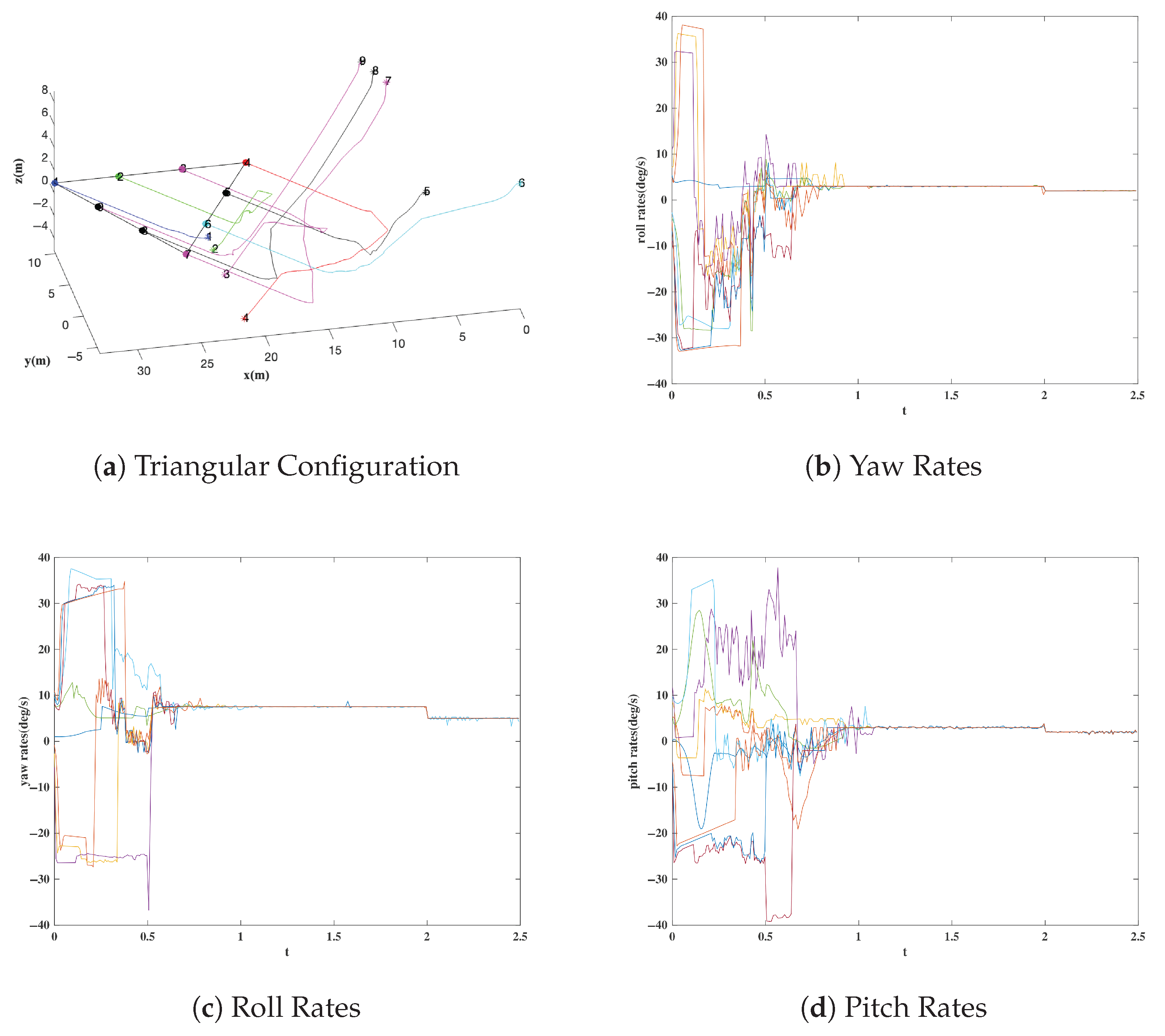
  • Case 1: Triangular Configuration Formation
In this simulation, nine NSVs are directed to form a configuration in the shape of an equilateral triangular. Starting from randomly assigned attitude angles, the control algorithm ensures that the communication network satisfies the minimal angle rigidity requirement, which mandates 20 angle constraints. This algorithm effectively guarantees that the formation remains stable, precise, and consistently robust.
The initial attitude angles for the NSVs are x 1 = [ 1 18 π ,   1 50 π ,   1 36 π ] T , x 2 = [ 2 45 π ,   1 60 π ,   1 36 π ] T , x 3 = [ 1 45 π ,   1 90 π ,   1 36 π ] T ,   x 4 = [ 1 60 π ,   1 45 π ,   1 36 π ] T , x 5 = [ 1 45 π ,   1 60 π ,   1 36 π ] T , x 6 = [ 1 30 π ,   1 90 π ,   1 30 π ] T , x 7 = [ 1 18 π ,   1 36 π ,   7 180 π ] T ,   x 8 = [ 1 18 π ,   1 45 π ,   2 45 π ] T , and x 9 = [ 1 18 π ,   1 60 π ,   1 20 π ] T . The simulation results (Figure 3) confirmed the successful transition of the NSVs to a triangular formation, with the attitude angles gradually aligning to zero and indicating coordinated movement.
  • Case 2: Hexagonal Configuration Formation
This scenario explores the control of 12 NSVs as they achieve a stable three-dimensional hexagonal configuration. The formation process is guided by a communication network that is carefully constructed to meet the minimal angle rigidity criterion, which dictates that the NSVs begin with the following initial attitude angles: x 1 = [ 1 18 π ,   0 ,   1 18 π ] T , x 2 = [ 2 45 π ,   1 90 π ,   2 45 π ] T , x 3 = [ 1 30 π ,   1 36 π ,   1 18 π ] T , x 4 = [ 1 45 π ,   1 36 π ,   2 45 π ] T ,   x 5 = [ 1 36 π ,   1 45 π ,   1 18 π ] T , x 6 = [ 1 20 π ,   1 60 π ,   0 ] T , x 7 = [ 1 18 π ,   1 36 π ,   0 ] T ,   x 8 = [ 7 180 π ,   1 45 π ,   0 ] T , x 9 = [ 1 30 π ,   1 36 π ,   0 ] T , x 10 = [ 1 15 π ,   1 36 π ,   0 ] T , x 11 = [ 1 18 π ,   1 36 π ,   1 60 π ] T , x 12 = [ 2 45 π ,   1 45 π ,   0 ] T .
As shown in Figure 4, the NSVs effectively achieve the desired hexagonal configuration, with their attitude angle rates converging to a common value, thereby exhibiting synchronized motion. This confirms the stability and effectiveness of the proposed control algorithm in maintaining coordinated formation.
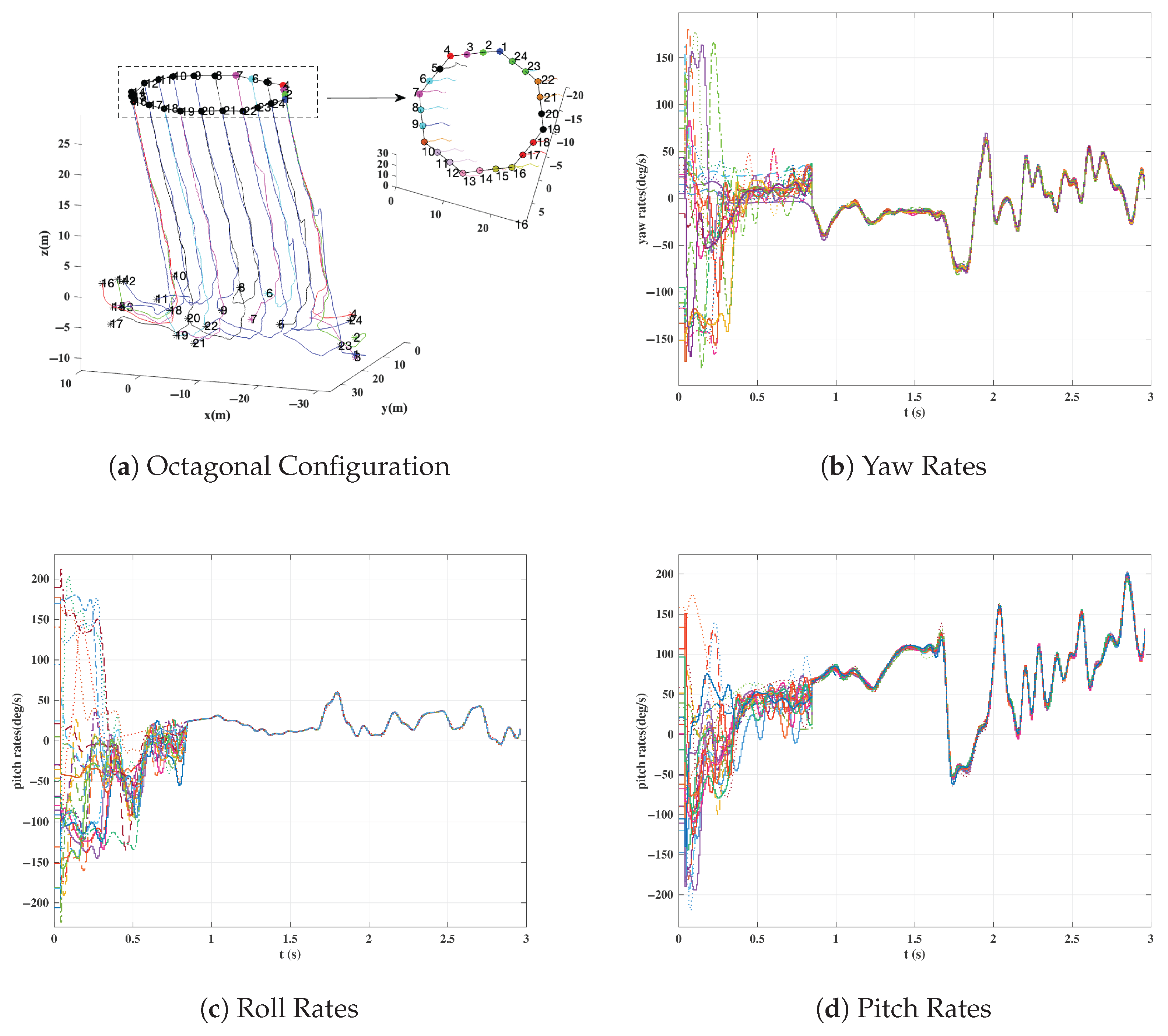
  • Case 3: Octagonal Configuration Formation
This case investigates the formation control of 24 NSVs arranged in a three-dimensional octagonal configuration. Each NSV begins with a randomly assigned initial attitude, and the goal of formation control is to guide the NSVs into the desired octagonal formation.
The initial attitude angles for the system are specifically set as follows: x 1 = [ 1 6 π ,   1 45 π ,   1 18 π ] T , x 2 = [ 29 180 π ,   1 60 π ,   2 45 π ] T , x 3 = [ 14 90 π ,   1 40 π ,   1 15 π ] T , x 4 = [ 13 90 π ,   2 45 π ,   1 30 π ] T , x 5 = [ 2 30 π ,   1 60 π ,   1 18 π ] T , x 6 = [ 1 18 π ,   1 50 π ,   1 36 π ] T ,   x 7 = [ 2 45 π ,   1 60 π ,   1 20 π ] T , x 8 = [ 1 30 π ,   1 45 π ,   1 45 π ] T , x 9 = [ 1 60 π ,   1 40 π ,   2 45 π ] T , x 10 = [ 1 36 π ,   1 60 π ,   1 60 π ] T ,   x 11 = [ 2 45 π ,   1 50 π ,   7 180 π ] T , x 12 = [ 1 18 π ,   1 60 π ,   1 90 π ] T , x 13 = [ 1 18 π ,   2 45 π ,   1 30 π ] T , x 14 = [ 1 18 π ,   1 40 π ,   1 180 π ] T ,   x 15 = [ 1 18 π ,   1 45 π ,   1 36 π ] T ,   x 16 = [ 1 18 π ,   1 50 π ,   0 ] T , x 17 = [ 1 36 π ,   1 60 π ,   1 45 π ] T , x 18 = [ 1 36 π ,   1 45 π ,   1 180 π ] T ,   x 19 = [ 1 30 π ,   1 50 π ,   1 36 π ] T , x 20 = [ 2 45 π ,   1 60 π ,   1 90 π ] T , x 21 = [ 1 20 π ,   1 45 π ,   1 30 π ] T , x 22 = [ 11 180 π ,   1 60 π ,   1 60 π ] T , x 23 = [ 1 6 π ,   2 45 π ,   7 180 π ] T , x 24 = [ 1 6 π ,   1 50 π ,   1 45 π ] T .
The simulation results, which are displayed in Figure 5, demonstrate that the NSVs successfully formed the octagonal configuration. Each NSV began with a randomly assigned initial attitude. The control mechanism ensured that the communication framework adhered to the minimal A rigidity condition, and it required 65 angle constraints for structural integrity. The convergence of the attitude angles further validated the effectiveness of the control strategy in achieving and maintaining this complex formation.

7. Conclusions

This paper introduces an advanced formation control strategy for near-space vehicles (NSVs) that effectively addresses actuator dead zones, input saturation, and external disturbances. By integrating angle rigidity formation control, neural networks, and adaptive estimation techniques, the proposed method enhances the robustness and precision of NSV formation control in dynamic environments. The stability analysis based on Lyapunov theory validates the effectiveness of this approach, as evidenced by successful simulation results demonstrating the system’s ability to maintain desired formations despite uncertainties. Future research could focus on refining these techniques to further reduce computational overhead and improve response times, thereby extending the applicability of the strategy to more demanding missions.

Author Contributions

Q.W.: Conceptualization, formal analysis, supervision, validation, writing—review and editing. Y.S.: Conceptualization, data curation, formal analysis, methodology, software, visualization, writing—original draft. H.Y.: Data curation, investigation, visualization. J.Y.: Methodology, validation, writing—review and editing. Y.Y.: Funding acquisition, project administration, resources, supervision, writing—review and editing. All authors have read and agreed to the published version of the manuscript.

Funding

This work was supported by the National Natural Science Foundation of China under Grants 92371116 and 62433005, and by the Postgraduate Research & Practice Innovation Program of Jiangsu Province (KYCX25_3971).

Informed Consent Statement

Not applicable.

Data Availability Statement

The original contributions presented in the study are included in the article; further inquiries can be directed to the corresponding author.

Conflicts of Interest

The authors declare that the research was conducted in the absence of any commercial or financial relationships that could be construed as a potential conflict of interest.

Acronyms and Notations

Acronyms
MIMOMulti-Input Multi-Output
NNNeural Networks
NSVNear-Space Vehicle
RBFRadial Basis Function
RBFNNRadial Basis Function Neural Network
Notation
α Angle of attack [rad]
α i l 
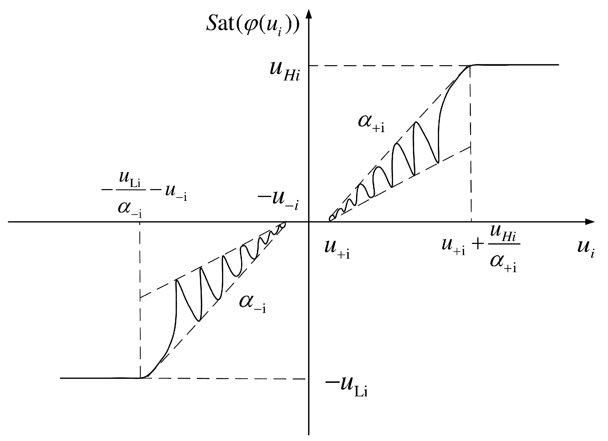
Saturation slope for l-th component of i-th NSV, min { α i l , α + i l }
α + i l Positive saturation slope for l-th component
α i l Negative saturation slope for l-th component
β Sideslip angle [rad]
b Spread of -th RBF [dimensionless]
C L , α Lift coefficient derivative w.r.t. angle of attack
C Y , β Side force coefficient derivative w.r.t. sideslip angle
d i ( t ) External disturbance for i-th NSV [rad/s2]
d f ( t ) Fast-loop disturbance [rad/s2]
d s ( t ) Slow-loop disturbance [rad/s2]
D i Bound on d i ( t ) [rad/s2]
δ a Aileron deflection [rad]
δ c Control deflections, [ δ e , δ a , δ r ] T [rad]
δ e Elevator deflection [rad]
δ i RBFNN approximation error [rad/s2]
δ i ¯ Bound on | δ i | [rad/s2]
δ r Rudder deflection [rad]
Δ u i Saturation error, Sat ( φ i ( u i ) ) φ i ( u i ) [rad/s2]
Δ u i M Bound on Δ u i [rad/s2]
eEdge vector, e = H ¯ x [rad]
EEdge set of graph G
f i ( x i ) Nonlinear dynamics for i-th NSV [rad/s2]
f s Slow-loop dynamics, [ f α , f β , f μ ] T [rad/s2]
f α Dynamics for angle of attack [rad/s2]
f β Dynamics for sideslip angle [rad/s2]
f μ Dynamics for bank angle [rad/s2]
gGravitational acceleration [m/s2]
g i ( x i ) Control gain matrix for i-th NSV
g s ( Ω ) Slow-loop gain matrix, g 1
g f ( ω ) Fast-loop gain matrix, K 1 [s2/kg·m2]
g 1 Attitude rate coupling matrix
g 2 Control effectiveness matrix [rad/s2]
g α , δ e Elevator effect on angle of attack [rad/s2]
g α , δ a Aileron effect on angle of attack [rad/s2]
g α , δ r Rudder effect on angle of attack [rad/s2]
g β , δ e Elevator effect on sideslip angle [rad/s2]
g β , δ a Aileron effect on sideslip angle [rad/s2]
g β , δ r Rudder effect on sideslip angle [rad/s2]
g μ , δ e Elevator effect on bank angle [rad/s2]
g μ , δ a Aileron effect on bank angle [rad/s2]
g μ , δ r Rudder effect on bank angle [rad/s2]
GTopology graph, G = ( V , E )
G Directed topology graph
h i Disturbance bound [rad/s2]
h ^ i Estimated disturbance bound [rad/s2]
h i Dead-zone parameter vector, components h i l = α i l u ¯ i l [rad/s2]
h ˜ i Disturbance plus error, δ i + d i [rad/s2]
h f ( ω ) Fast-loop dynamics, K 1 Ω ( ω ) K ω [rad/s2]
h s ( Ω ) Slow-loop dynamics, f s [rad/s2]
H ( G ) Incidence matrix, ( h i j ) R m × n
H ¯ Kronecker product, H I n
H 0 NSV altitude [m]
I n n × n identity matrix
J i ( t ) Control magnitude for i-th NSV [rad/s2]
KNSV inertia matrix [kg·m2]
L ( 0 , 1 ) 3 3D standard normal random vector
λ i Adaptive gain for RBFNN weights
λ i j Component of λ i
| λ ( g i ( x i ) ) | m i n Minimum eigenvalue of g i ( x i )
MNSV mass [kg]
M C ( t ) Control torque, g 2 δ c [N·m]
μ Bank angle [rad]
μ i l Center of l-th RBF [rad]
N i Neighbor set of i-th NSV
ν RBF center, [ 0.01 ( 5 ) , 0.01 ( 5 ) , 0.01 ( 5 ) ] T [rad]
η i Adaptive gain for disturbance estimation
η i j Component of η i
Ω Attitude angles, [ α , β , μ ] T [rad]
pRoll rate [rad/s]
ϕ i ( χ i ) RBF vector for i-th NSV
φ i ( u i ) Saturation model input [rad/s2]
Φ i l ( χ i ) l-th RBF, exp χ i μ i l 2 ( σ i l ) 2
ψ ( u ) Saturated control, Sat ( φ ( u ) ) [rad/s2]
qPitch rate [rad/s]
q ^ Dynamic pressure [kg/(m·s2)]
rYaw rate [rad/s]
r f Fast-loop input, M C [N·m]
r s Slow-loop input, ω [rad/s]
SNSV reference area [m2]
σ i l Spread of l-th RBF [rad]
Sat ( φ i ( u i ) ) Saturated control output [rad/s2]
θ i RBFNN optimal weights
θ ^ i Estimated RBFNN weights
T x Thrust in body x-axis [N]
T y Thrust in body y-axis [N]
u i Control input for i-th NSV [rad/s2]
u ¯ i Max dead-zone threshold, max { u i , u + i } [rad/s2]
u + i l Positive dead-zone threshold [rad/s2]
u i l Negative dead-zone threshold [rad/s2]
u H i l Upper saturation limit [rad/s2]
u L i l Lower saturation limit [rad/s2]
VNode set of graph G
V A NSV airspeed [m/s]
vConcatenated velocity, [ v 1 T , , v n T ] T [rad/s]
V i Potential energy for i-th NSV [dimensionless]
V i j Potential energy between NSVs i and j
V 0 Initial NSV speed [m/s]
W ( t ) Lyapunov function
x i ( t ) Attitude angles for i-th NSV [rad]
x f Fast-loop state, ω [rad/s]
x s Slow-loop state, Ω [rad]
x i j Relative attitude, x i x j [rad]
x i j Target relative attitude [rad]
χ i RBFNN input vector [rad]
y i ( t ) Output of i-th NSV, x i [rad]
y f ( t ) Fast-loop output, ω [rad/s]
y s ( t ) Slow-loop output, Ω [rad]

References

  1. Sun, C.; Mu, C.; Yu, Y. Some Control Problems for Near Space Hypersonic Vehicles. Acta Autom. Sin. 2013, 39, 1901. [Google Scholar] [CrossRef]
  2. Dong, Z.; Lv, M.; Da, X.; Zhang, Q. Neuro-Adaptive Singularity-Free Fixed-Time Constrained Trajectory Tracking Control of HFVs With Specified Accuracy. Int. J. Robust Nonlinear Control 2025, 35, 3545–3558. [Google Scholar] [CrossRef]
  3. Dong, Z.; Li, Y.; Lv, M. Adaptive nonsingular fixed-time control for hypersonic flight vehicle considering angle of attack constraints. Int. J. Robust Nonlinear Control 2023, 33, 6754–6777. [Google Scholar] [CrossRef]
  4. Zhang, S.; Li, X.; Zuo, J.; Qin, J.; Cheng, K.; Feng, Y.; Bao, W. Research progress on active thermal protection for hypersonic vehicles. Prog. Aerosp. Sci. 2020, 119, 100646. [Google Scholar] [CrossRef]
  5. Aslam, M.S.; Tiwari, P.; Pandey, H.M.; Band, S.S. Robust stability analysis for class of Takagi-Sugeno (T-S) fuzzy with stochastic process for sustainable hypersonic vehicles. Inf. Sci. 2023, 641, 119044. [Google Scholar] [CrossRef]
  6. Xia, R.; Chen, M.; Wu, Q.; Wang, Y. Neural network based integral sliding mode optimal flight control of near space hypersonic vehicle. Neurocomputing 2020, 379, 41–52. [Google Scholar] [CrossRef]
  7. Wu, X.; Wei, C.; Chen, T.; Dai, M.Z. On novel distributed fixed-time formation tracking of multiple hypersonic flight vehicles with collision avoidance. Aerosp. Sci. Technol. 2023, 141, 108517. [Google Scholar] [CrossRef]
  8. Lv, M.; De Schutter, B.; Baldi, S. Nonrecursive Control for Formation-Containment of HFV Swarms With Dynamic Event-Triggered Communication. IEEE Trans. Ind. Inform. 2023, 19, 3188–3197. [Google Scholar] [CrossRef]
  9. Yi, X.; Yu, H.; Xu, T. Solving multi-objective weapon-target assignment considering reliability by improved MOEA/D-AM2M. Neurocomputing 2024, 563, 126906. [Google Scholar] [CrossRef]
  10. Liu, Y.; Ma, G.; Lyu, Y.; Wang, P. Neural network-based reinforcement learning control for combined spacecraft attitude tracking maneuvers. Neurocomputing 2022, 484, 67–78. [Google Scholar] [CrossRef]
  11. Liu, R.; Cao, X.; Liu, M.; Zhu, Y. 6-DOF fixed-time adaptive tracking control for spacecraft formation flying with input quantization. Inf. Sci. 2019, 475, 82–99. [Google Scholar] [CrossRef]
  12. Feng, J.; Song, W.; Xu, L.; Zhang, J. Formation control of multiagent systems with multileaders through completely distributed intermittent communication strategies. Inf. Sci. 2025, 690, 121555. [Google Scholar] [CrossRef]
  13. Li, A.; Liu, M.; Cao, X.; Liu, R. Adaptive quantized sliding mode attitude tracking control for flexible spacecraft with input dead-zone via Takagi-Sugeno fuzzy approach. Inf. Sci. 2022, 587, 746–773. [Google Scholar] [CrossRef]
  14. Dong, H.; Yang, X. Learning-based online optimal sliding-mode control for space circumnavigation missions with input constraints and mismatched uncertainties. Neurocomputing 2022, 484, 13–25. [Google Scholar] [CrossRef]
  15. Xiao, Y.; Li, Y.; Liu, H.; Chen, Y.; Wang, Y.; Wu, G. Adaptive large neighborhood search algorithm with reinforcement search strategy for solving extended cooperative multi task assignment problem of UAVs. Inf. Sci. 2024, 679, 121068. [Google Scholar] [CrossRef]
  16. Fabris, M.; Fattore, G.; Cenedese, A. Optimal time-invariant distributed formation tracking for second-order multi-agent systems. Eur. J. Control 2024, 77, 100985. [Google Scholar] [CrossRef]
  17. Wang, P.-F.; Chang, L.; Yan, B. Development of Near Space Hypersonic Vehicles and Defense Strategies Analysis. Mod. Def. Technol. 2021, 49, 16. [Google Scholar]
  18. Chen, K.; Pei, S.S.; Zeng, C.Z. SINS/BDS tightly coupled integrated navigation algorithm for hypersonic vehicle. Sci. Rep. 2022, 12, 6144. [Google Scholar] [CrossRef]
  19. Smith, T.K.; Akagi, J.; Droge, G. Model predictive control for formation flying based on D’Amico relative orbital elements. Astrodynamics 2025, 9, 143–163. [Google Scholar] [CrossRef]
  20. Xu, B.; Shou, Y.; Shi, Z.; Yan, T. Predefined-Time Hierarchical Coordinated Neural Control for Hypersonic Reentry Vehicle. IEEE Trans. Neural Netw. Learn. Syst. 2023, 34, 8456–8466. [Google Scholar] [CrossRef]
  21. Wang, J.; Zhang, C.; Zheng, C.; Kong, X.; Bao, J. Adaptive neural network fault-tolerant control of hypersonic vehicle with immeasurable state and multiple actuator faults. Aerosp. Sci. Technol. 2024, 152, 109378. [Google Scholar] [CrossRef]
  22. Sun, X.; Wang, Y.; Su, J.; Li, J.; Xu, M.; Bai, S. Relative orbit transfer using constant-vector thrust acceleration. Acta Astronaut. 2025, 229, 715–735. [Google Scholar] [CrossRef]
  23. Chen, M.; Yu, J. Disturbance observer-based adaptive sliding mode control for near-space vehicles. Nonlinear Dyn. 2015, 82, 1671–1682. [Google Scholar] [CrossRef]
  24. Cheng, L.; Jiang, C.; Pu, M. Online-SVR-compensated nonlinear generalized predictive control for hypersonic vehicles. Sci. China Inf. Sci. 2011, 54, 551–562. [Google Scholar] [CrossRef]
  25. Dong, W.; Qi, R.; Jiang, B. Composite fault tolerant control for aerospace vehicles with swing engines and aerodynamic fins. Acta Aeronaut. Astronaut. Sin. 2020, 41, 623850. [Google Scholar]
  26. Cheng, L.; Wang, Z.; Gong, S. Adaptive control of hypersonic vehicles with unknown dynamics based on dual network architecture. Acta Astronaut. 2022, 193, 197–208. [Google Scholar] [CrossRef]
  27. Zhao, K.; Song, J.; Ai, S.; Xu, X.; Liu, Y. Active Fault-Tolerant Control for Near-Space Hypersonic Vehicles. Aerospace 2022, 9, 237. [Google Scholar] [CrossRef]
  28. Zhu, S.; Xu, T.; Wei, C.; Wang, Z. Learning-based adaptive fault tolerant control for hypersonic flight vehicles with abrupt actuator faults and finite time prescribed tracking performance. Eur. J. Control 2021, 58, 17–26. [Google Scholar] [CrossRef]
  29. Du, Y.; Wu, Q.; Jiang, C.; Wen, J. Adaptive functional link network control of near-space vehicles with dynamical uncertainties. J. Syst. Eng. Electron. 2010, 21, 868–876. [Google Scholar] [CrossRef]
  30. Yu, J.; Shi, P.; Dong, W.; Lin, C. Adaptive Fuzzy Control of Nonlinear Systems With Unknown Dead Zones Based on Command Filtering. IEEE Trans. Fuzzy Syst. 2018, 26, 46–55. [Google Scholar] [CrossRef]
  31. Chen, M.; Ren, B.; Wu, Q.; Jiang, C. Anti-disturbance control of hypersonic flight vehicles with input saturation using disturbance observer. Sci. China Inf. Sci. 2015, 58, 1–12. [Google Scholar] [CrossRef]
  32. Zhao, S.; Zelazo, D. Bearing-based formation maneuvering. In Proceedings of the 2015 IEEE International Symposium on Intelligent Control (ISIC), Sydney, Australia, 21–23 September 2015; pp. 658–663. [Google Scholar]
  33. Chen, M.; Wu, Q.; Jiang, C.; Jiang, B. Guaranteed transient performance based control with input saturation for near space vehicles. Sci. China Inf. Sci. 2014, 57, 1–12. [Google Scholar] [CrossRef]
  34. Zhang, Y.; Wang, X.; Tang, S. A globally fixed-time solution of distributed formation control for multiple hypersonic gliding vehicles. Aerosp. Sci. Technol. 2020, 98, 105643. [Google Scholar] [CrossRef]
  35. Zuo, R.; Li, Y.; Lv, M.; Dong, Z. Learning-Based Distributed Containment Control for HFV Swarms Under Event-Triggered Communication. IEEE Trans. Aerosp. Electron. Syst. 2023, 59, 568–579. [Google Scholar] [CrossRef]
  36. Zhou, H.; Jiao, B.; Dang, Z.; Yuan, J. Parametric formation control of multiple nanosatellites for cooperative observation of China Space Station. Astrodynamics 2024, 8, 77–95. [Google Scholar] [CrossRef]
  37. Zou, A.M.; Kumar, K.D. Neural Network-Based Distributed Attitude Coordination Control for Spacecraft Formation Flying With Input Saturation. IEEE Trans. Neural Netw. Learn. Syst. 2012, 23, 1155–1162. [Google Scholar]
  38. Sun, H.J.; Wu, Y.Y.; Zhang, J. A distributed predefined-time attitude coordination control scheme for multiple rigid spacecraft. Aerosp. Sci. Technol. 2023, 133, 108134. [Google Scholar] [CrossRef]
  39. Zhuang, M.; Tan, L.; Song, S. Fixed-time attitude coordination control for spacecraft with external disturbance. ISA Trans. 2021, 114, 150–170. [Google Scholar] [CrossRef]
  40. Chen, M.; Jiang, B. Robust attitude control of near space vehicles with time-varying disturbances. Int. J. Control Autom. Syst. 2013, 11, 182–187. [Google Scholar] [CrossRef]
  41. Guo, Z.; Guo, J.; Zhou, J.; Chang, J. Robust Tracking for Hypersonic Reentry Vehicles via Disturbance Estimation-Triggered Control. IEEE Trans. Aerosp. Electron. Syst. 2020, 56, 1279–1289. [Google Scholar] [CrossRef]
  42. Xia, R.; Bu, C.; Yan, X.; Zhou, T. Finite-horizon optimal trajectory control of near space hypersonic vehicle with multi-constraints. Optim. Control Appl. Methods 2024, 45, 302–320. [Google Scholar] [CrossRef]
  43. Xi, C.; Dong, J. Adaptive neural network-based control of uncertain nonlinear systems with time-varying full-state constraints and input constraint. Neurocomputing 2019, 357, 108–115. [Google Scholar] [CrossRef]
  44. Zou, Y.; Zheng, Z. A Robust Adaptive RBFNN Augmenting Backstepping Control Approach for a Model-Scaled Helicopter. IEEE Trans. Control Syst. Technol. 2015, 23, 2344–2352. [Google Scholar] [CrossRef]
  45. Zhao, S.; Zelazo, D. Bearing Rigidity and Almost Global Bearing-Only Formation Stabilization. IEEE Trans. Autom. Control 2016, 61, 1255–1268. [Google Scholar] [CrossRef]
  46. Buckley, I.; Egerstedt, M. Infinitesimal Shape-Similarity for Characterization and Control of Bearing-Only Multirobot Formations. IEEE Trans. Robot. 2021, 37, 1921–1935. [Google Scholar] [CrossRef]
  47. Chen, L.; Cao, M. Angle Rigidity for Multiagent Formations in 3-D. IEEE Trans. Autom. Control 2023, 68, 6130–6145. [Google Scholar] [CrossRef]
Figure 1. Sat ( φ i ( u i ) ) with dead zone and saturation effects.
Actuators 14 00339 g001
Figure 2. Control structure block diagram.
Actuators 14 00339 g002
Figure 3. Simulation results for triangular configuration formation. (a) Triangular configuration. (b) Yaw rates. (c) Roll rates. (d) Pitch rates.
Actuators 14 00339 g003
Figure 4. Simulation results for hexagonal configuration formation. (a) Hexagonal configuration. (b) Yaw rates. (c) Roll rates. (d) Pitch rates.
Actuators 14 00339 g004
Figure 5. Simulation results for octagonal configuration formation. (a) Octagonal configuration. (b) Yaw rates. (c) Roll rates. (d) Pitch rates.
Actuators 14 00339 g005
Disclaimer/Publisher’s Note: The statements, opinions and data contained in all publications are solely those of the individual author(s) and contributor(s) and not of MDPI and/or the editor(s). MDPI and/or the editor(s) disclaim responsibility for any injury to people or property resulting from any ideas, methods, instructions or products referred to in the content.

