Hysteresis Modeling of Soft Pneumatic Actuators: An Experimental Review

Abstract

Hysteresis is a nonlinear phenomenon found in many physical systems, including soft viscoelastic actuators, where it poses significant challenges to their application and performance. Consequently, developing accurate hysteresis models is essential for the effective design and optimization of soft actuators. Moreover, a reliable model can be used to design compensators that mitigate the negative effects of hysteresis, improving closed-loop control accuracy and expanding the applicability of soft actuators in robotics. Physics-based approaches for modeling hysteresis in soft actuators offer valuable insights into the underlying material behavior. Nevertheless, they are often highly complex, making them impractical for real-world applications. Instead, phenomenological models provide a more feasible solution by representing hysteresis through input–output mappings based on experimental data. To effectively fit these phenomenological models, it is essential to rely on sensing data collected from real actuators. In this context, the primary objective of this work is a comprehensive comparative evaluation of the efficiency and performance of representative phenomenological hysteresis models (e.g., Bouc–Wen and Prandtl-Ishlinskii) using experimental data obtained from a pneumatic bending actuator made of a viscoelastic material. This evaluation suggests that the Generalized Prandtl–Ishlinskii model achieves the highest modeling accuracy, while the Preisach model with a probabilistic density function formulation excels in terms of parameter compactness.

1. Introduction

As soft robotics advances toward a range of applications—such as assistive and wearable devices [1,2], surgical assistance [3,4,5], collaborative robots [6], rescue missions [7,8] and exploration [9]—the development of compliant and robust actuators becomes essential. However, inherent nonlinear characteristics of soft actuators, such as hysteresis, can limit their performance [10,11].

Hysteresis arises naturally in a wide range of disciplines, from material science to mechanics, magnetism and even biological systems. Notably, smart materials, which are extensively used in soft robotics, ubiquitously exhibit hysteresis [12,13].

In soft pneumatic actuators, hysteresis appears due to multiple factors: energy dissipation during deformation in viscoelastic materials [14,15]; frictional losses between the surfaces of pneumatic chambers and other components added to guide deformations, such as braided shells [16,17] and even from nonlinearities coming from the pneumatic system itself [18,19]. Therefore, a thorough study and modeling of the hysteretic characteristics of soft actuators and their materials is an essential step toward their optimal design and control.

As [20] remarks, the definition of hysteresis varies across different fields, papers and authors. Commonly, a hysteretic behavior is defined as a nonlinear phenomenon in which the response of a system depends not only on the current input but also on its past inputs, resulting in different paths during loading and unloading. Sometimes, the word hysteresis connotes lag, although this definition is misleading, since delay, per se, is not the mechanism that produces hysteresis. In fact, most dynamical systems (even linear) exhibit lag or phase shift with high enough frequencies, obtaining closed loops that behave as Lissajous-type loops [21]. In contrast, a pure hysteretic behavior appears even when input signals become slower and slower, producing a nontrivial input–output loop that persists in the static limit and that is unrelated with phase shifts [12,21,22].

Hysteresis models are categorized into three main groups: physics-based, data-driven and phenomenological. Physics-based models are derived using first principles along with particular material properties to capture the hysteresis within a system. One example is the Jiles–Atherton model, used to describe ferromagnetic hysteresis [23]. However, physics-based models are usually too complex to be used in practical applications. In general, engineering practice seeks simpler models that keep relevant input–output features and are useful for characterization, design and control purposes [24].

Data-driven methods have also been widely applied to characterize hysteretic behavior in dynamical systems. Among these approaches, there are regression-based techniques, such as the Auto-Regressive model with Exogenous inputs (ARX) and the Auto-Regressive Moving Average (ARMA) model [25]. More recently, deep learning algorithms have gained attraction. For example, Recurrent Neural Networks (RNNs) have been trained to model and compensate hysteresis loops [26]. Gaussian processes offer another powerful probabilistic approach, enabling both output representation and uncertainty quantification in hysteretic systems [27]. In addition to these, a broad spectrum of other data-driven strategies has also been explored [28].

However, while powerful, data-driven methods typically require large amounts of hysteresis data for accurate modeling. Moreover, their general black-box structure complicates both the interpretability and the adaptation of these models across different systems.

Phenomenological models, on the other hand, aim to describe hysteresis through explicit mathematical mappings between inputs and outputs. These models are classified into two types:

• Models that use differential equations to characterize hysteresis, for instance, the Bouc–Wen model, which employs a nonlinear differential equation to represent hysteretic systems with a wide range of shapes [29].
• Models that use a composition of weighted hysteresis-like operators, such as the Maxwell-Slip model, a dynamic friction model commonly represented as a parallel connection of frictional sliders and springs [30], the Preisach model, which has been mainly used for describing static magnetic behavior [31], and the Prandtl–Ishlinskii model, which has been very popular in a wide range of systems for its simplicity and flexibility [32].

Because phenomenological models capture intrinsic hysteretic properties, they are easier to identify. Also, their general and explicit mathematical formulation facilitates their integration with other systems and methods. For example, in [33] a Nonlinear Auto-Regressive Moving Average model with Exogenous inputs (NARMAX) is combined with an improved Bouc–Wen model to model and control a magnetic shape memory alloy actuator.

Given the wide variety of phenomenological hysteresis models, and the fact that most works focus on only one or two, it can be challenging for researchers new to hysteresis modeling to determine which one is most relevant to their work. Furthermore, most of the review works on hysteresis, for example, [28,34,35,36], do not offer practical, side-by-side comparisons of the models.

Based on the above, the objectives of this work are as follows:

• To describe the key features and variants of various widely used phenomenological models, providing a clearer understanding of their underlying ideas.
• To serve as a tutorial for engineers and researchers interested in modeling hysteretic soft actuators by relating various commonly observed phenomena in hysteresis loops—such as asymmetry, the loading curve and the direction of hysteresis—to the mathematical structures and underlying concepts of each model.
• To present a direct comparison of the models after fitting them with real experimental data from a soft pneumatic bending actuator. Through this comparison, we aim to provide insights into the strengths and limitations of each model, while evaluating the accuracy, complexity (e.g., number of parameters) and computational efficiency.
• To assess which hysteresis models perform better or worse when applied to similar soft pneumatic bending actuators, thereby helping in the identification of trends across comparable systems.

The remainder of the paper is organized as follows. Section 2 outlines the methodology, including the experimental setup, data acquisition and preprocessing, optimization algorithms and performance metrics. Section 3, Section 4, Section 5 and Section 6 present and evaluate the Preisach, Prandtl–Ishlinskii, Maxwell-Slip and Bouc–Wen models, respectively, including notable variations. Section 7 discusses the conclusions derived through a comparative analysis of the models, and Section 8 provides a final discussion.

2. Methodology

2.1. Experimental Setup

The experimental data used in this study comes from the hydrogel-based pneumatic bending actuator developed in [37], which is depicted in Figure 1a. This actuator is composed of two different parts: a hollow cylindrical chamber made of CANESHA hydrogel and a surrounding reinforcement 3D-printed in TPU Recreus™Filaflex®82A (manufactured by Recreus Industries, Elda, Spain). The objective of the reinforcement is to prevent an excessive deformation of the hydrogel chamber when pressurized, guiding the movement of the actuator to obtain a specific bending motion (Figure 1b).

To measure the position of the actuator, its curvature $\kappa \ge 0$ is captured using a vision setup. A camera is placed after an illumination ring, to ensure that light conditions are the same between experiments (Figure 1c). A calibration checkerboard is used to correct the perspective deformations of the images. Then, captured images are processed to detect several green markers placed along the actuator (see Figure 1b), and, lastly, $\kappa$ is calculated as the inverse of the radius of the circumference that best fits these markers.

The pneumatic system, shown schematically in Figure 1d, has as its source an air compressor (model Stanley DST 100/8/6, manufactured by Stanley Black & Decker, New Britain, CT, USA). The pressurized air flows through a manual valve (model VHS30-F02B manufactured by SMC Corporation, Tokio, Japan) and a manual pressure regulator (model IR2010-F02, manufactured by SMC Corporation, Tokio, Japan), both used as a safety system. Downstream, an electronic pressure regulator model VEAB-L-26-D7-Q4-V1-1R1 manufactured by Festo AG, Esslingen am Neckar, Germany) and a solenoid valve (model EVT307-6DO-02F Q, manufactured by SMC Corporation, Tokio, Japan) (commanded by an electronic relay) modulate the air supply to the chamber of the actuator.

Both the electronic pressure regulator and the relay are controlled using a National Instruments^© CompactRIO cRIO-9024 device (manufactured by National Instruments Corporation, Austin, TX, USA). The CompactRIO is in charge of generating the input voltage signals that control the output pressure of the electronic regulator, while it simultaneously reads the internal pressure sensor of the regulator.

2.2. Data Acquisition, Preparation and Normalization

Since soft pneumatic bending actuators usually exhibit strong viscoelastic behaviors (e.g., the CANESHA hydrogel used for the actuator of this work), the signal used to excite the system must be slow enough (i.e., quasi-static) to capture only the pure hysteretic behavior of the system, without coupling with other phenomena. Thus, signals with a frequency $f=0.05\left[\mathrm{Hz}\right]$ were used. Higher-frequency excitations would introduce phase lag between the input and output, thereby distorting the characterization of the hysteresis loop.

For this class of systems, the actuator and the electronic pressure regulator can be viewed as a single “full actuator”, since the behavior of the regulator depends on what is downstream of it. Therefore, the system input $x\left(t\right)$ is the voltage signal applied to the electronic pressure regulator. As the regulator cannot work below atmospheric pressure, $x\left(t\right)$ must be always greater than zero. Therefore, a positive triangular signal is chosen as input:

$$x\left(t\right)=2\left|A\left(t·f-⌊t·f+{\displaystyle \frac{1}{2}}⌋\right)\right|,$$

(1)

where $\left|•\right|$ denotes the absolute value function and $⌊•⌋$ denotes the floor function. An amplitude $A=2\left[\mathrm{V}\right]$ was chosen to excite the system within a suitable range of motion. The full input signal is shown in Figure 2a, comprising four cycles to assess for the potential drift during operation.

The output signal (i.e., the curvature of the actuator) is shown in Figure 2b. After the initial loading, the actuator quickly stabilizes its behavior without a significant drift. Last but not least, since the actuator used in this work exhibits a slight curvature even at rest, the minimum value of the output signal is shifted by a constant offset.

In addition, the input and output signals have been normalized to the unit, presenting the hysteresis loop depicted in Figure 3. This normalization facilitates a direct comparison of the obtained model parameters with those of other works. As can be seen, the resulting hysteresis loop exhibits a strong asymmetric behavior, with a well-defined shape and an insignificant amount of noise.

2.3. Optimization Algorithm

To fit the compared models to the experimental data, we used the Genetic Algorithm (GA) provided by the MATLAB® Global Optimization Toolbox (using the function ga (https://es.mathworks.com/help/gads/ga.html, accessed on 26 June 2025)). Since our goal was not to fine-tune the GA parameters for hysteresis loop identification, we retained the default settings provided by the Global Optimization Toolbox, which proved sufficient for our purposes. To verify the convergence of the results, we repeated the optimization three times, each run yielding similar outcomes. The optimization problem consists in fitting the coefficients (each constrained with a maximum and minimum value) of each hysteresis model, minimizing the Root Mean Squared Error (RMSE):

$$\mathrm{RMSE}=\sqrt{{\displaystyle \frac{{\sum }_{i=1}^N{(y_i-{\widehat{y}}_i)}^2}{N}}}$$

(2)

in which N is the number of data points, ${\widehat{y}}_i$ is the simulated response from the fitted model and $y_i$ is the experimental output. Appendix A presents the coefficients and the simulation time of each model.

2.4. Comparison Metrics

To evaluate the models comparatively, we adopt as Goodness Of Fit (GOF) one minus the Normalized Root Mean Squared Error (NRMSE):

$$\mathrm{GOF}=1-\mathrm{NRMSE}=1-\sqrt{{\displaystyle \frac{{\sum }_{i=1}^N{(y_i-{\widehat{y}}_i)}^2}{{\sum }_{i=1}^N{(y_i-\overline{y})}^2}}}$$

(3)

where $\overline{y}$ is the mean of the whole experimental output signal $y\left(t\right)$. A GOF value closer to unity indicates a tighter match between the fitted model and measured data. Typically, GOF values above 0.95 are considered to reflect an excellent model fit, while values below 0.90 suggest that the model, although possibly capturing some essential behavior, may be inadequate for accurate representation or control purposes.

The following sections introduce various hysteresis models, highlighting their key concepts. Subsequently, we present the results of fitting each model using the methodology described above.

3. The Preisach Model

The Preisach model (PR) is one of the most popular operator-based models used to represent the nonlinear hysteretic behavior of systems. Originally, it was developed to represent magnetic hysteresis, which has been its main field of application [13,31]. However, because PR models can be specified purely in terms of mathematical formulations, they can be applied to a wide range of systems where the underlying physics are unknown. For example, they have been used to represent and compensate hysteresis in shape memory alloys [38] and pneumatic artificial muscles [39], to model piezoceramic [40] and piezoelectric actuators [41], to design robust and adaptive controllers [42] and even to characterize the seismic response of structures [43]. As a result, PR models have become a widely accepted mathematical tool for the description of hysteresis phenomena.

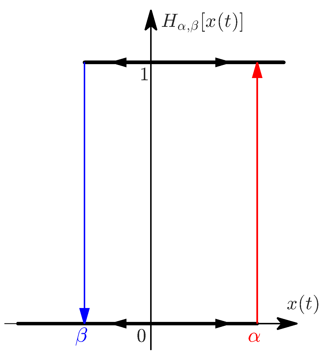
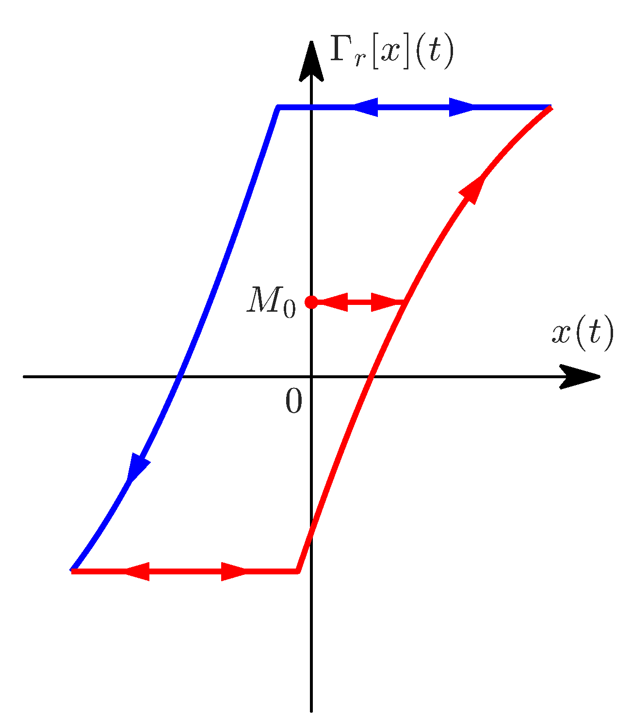
The PR model is based on the delayed relay operator $H_{\alpha ,\beta }[•]$ given by

$$H_{\alpha ,\beta }\left[x\left(t_k\right)\right]=\left\{\begin{array}{cc}1,\hfill & \mathrm{for}x\left(t_k\right)\ge \alpha \hfill \\ 0,\hfill & \mathrm{for}x\left(t_k\right)\le \beta \hfill \\ H_{\alpha ,\beta }\left[x\left(t_{k-1}\right)\right],\hfill & \mathrm{for}\beta <x\left(t_k\right)<\alpha \hfill \end{array}\right.$$

(4)

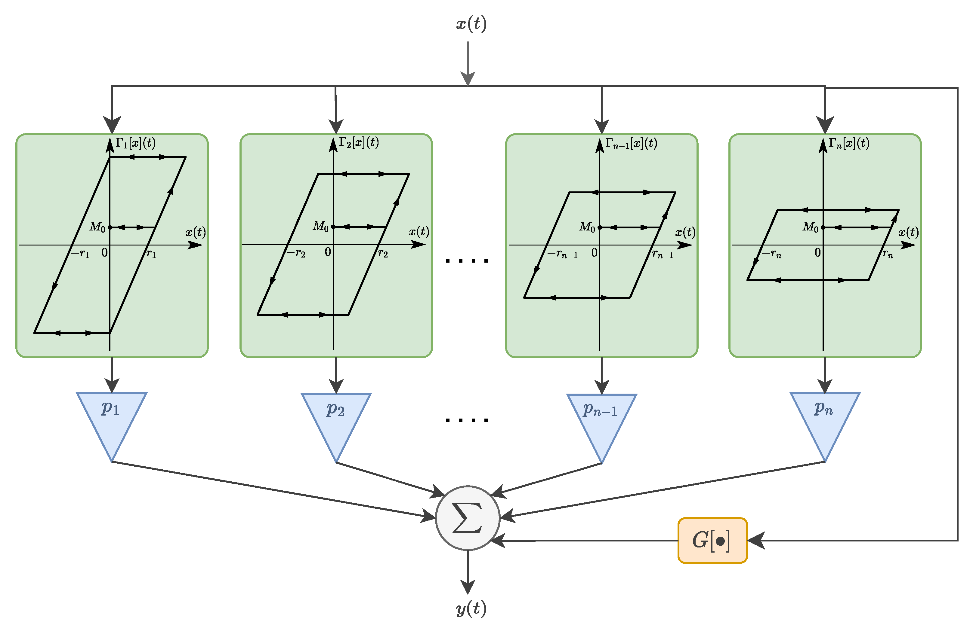
where $t_k=kh,k=1,2,\dots ,K$ is a time discretization of the input signal with a fixed step size h. The initial condition is $H_{\alpha ,\beta }\left[x\left(0\right)\right]=0$, and $\alpha ,\beta \in [min(x\left(t\right)),max(x\left(t\right)\left)\right]$ are, respectively, the upper and lower thresholds of the relay operator, shown in Figure 4. In this work, $\alpha ,\beta \in [0,1]$, as we use normalized data. The output of the PR model is obtained by summing many weighted relay operators connected in parallel, as illustrated in Figure 5. When the number of operators approaches infinity, the continuous PR model is obtained:

$${\Phi }_{PREI}\left[x\left(t\right)\right]=\int {\int }_{\alpha \ge \beta }p(\alpha ,\beta )H_{\alpha ,\beta }\left[x\left(t\right)\right]d\alpha d\beta$$

(5)

in which $p(\alpha ,\beta )\ge 0$ is the Preisach density function.

However, estimating the PR density function from hysteresis loops is a nontrivial task, and several methods have been developed to obtain it. Common approaches involve taking numerical derivatives of measurements. However, that can lead to significant errors if the data is noisy or poorly treated [44].

Another common approach is to approximate the PR density function by some analytical probability density function [45]. In this regard, some works aim to further simplify the identification of the density function. In this work, we adopt the solution of [46], where the PR function is assumed to be the product of two independent general probability distributions:

$$p(\alpha ,\beta )=p(H_M,H_C)=p\left(H_M\right)·p\left(H_C\right)$$

(6)

where $p\left(H_M\right)$ and $p\left(H_C\right)$ are two distributions with variables $H_M=(\alpha +\beta )/2$ and $H_C=(\alpha -\beta )/2$. These distributions are well-known continuous statistical distributions, such as the Gaussian $p{\left(k\right)}_{Gs}$ and Cauchy $p{\left(k\right)}_{Cy}$ distributions:

$$p{\left(k\right)}_{Gs}={\displaystyle \frac{1}{\sqrt{2\pi }{\sigma }_k}}·e^{-{\displaystyle \frac{{(k-{\mu }_k)}^2}{2{\sigma }_k^2}}}$$

(7)

$$p{\left(k\right)}_{Cy}={\displaystyle \frac{1}{\pi {\sigma }_k}}·{\displaystyle \frac{1}{1+{\left[(k-{\mu }_k)/{\sigma }_k\right]}^2}}$$

(8)

where the variable k represents $H_C$ or $H_M$, depending on the desired combination; ${\mu }_k\in \mathbb{R}$ is the center of the distribution and ${\sigma }_k\in \mathbb{R}$ its standard deviation. If, instead of the continuous PR model, N equally spaced thresholds for $\alpha$ and $\beta$ between $min\left(x\right(t\left)\right)$ and $max\left(x\right(t\left)\right)$ are considered, Equation (5) becomes

$${\Phi }_{PREI}\left[x\left(t\right)\right]=y_0+\sum _{i=1}^N\sum _{j=1}^{i}p(H_M,H_C)H_{{\alpha }_i,{\beta }_j}\left[x\left(t\right)\right]$$

(9)

where the limits of the summation ${\sum }_{j=1}^i$ are set to satisfy the condition $\alpha \ge \beta$. Additionally, the term $y_0$ is added to account for the offset in the experimental data.

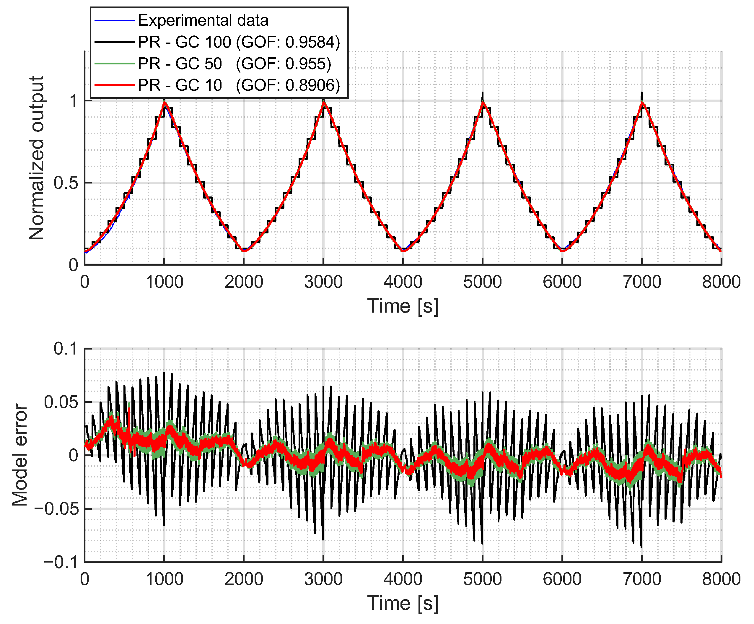
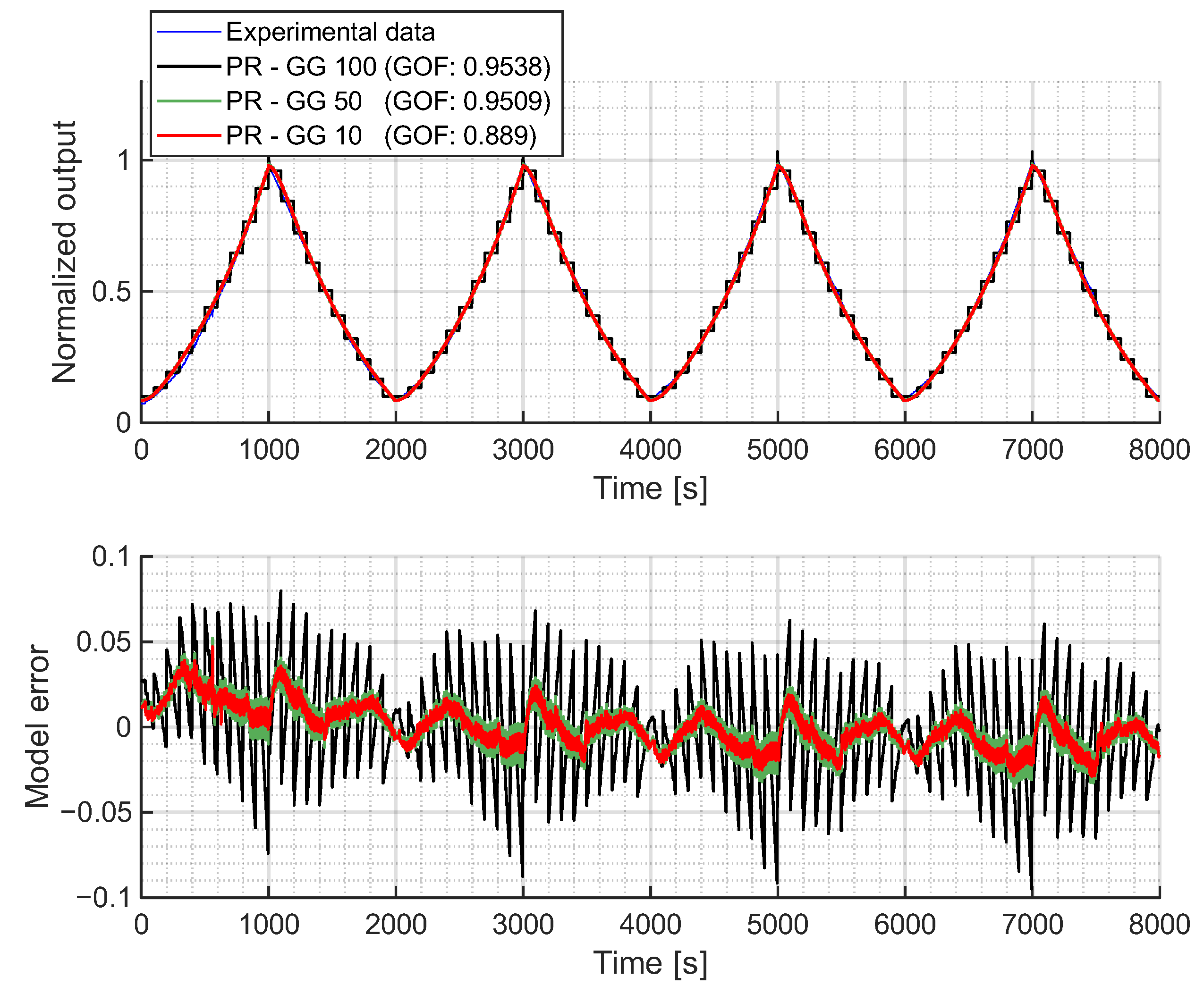
Fitting Results

In this section, the results of fitting the formulation of the PR model (9) are presented. This model was fitted with the GA explained in Section 2.3, applying two different combinations of the introduced probabilistic density functions (7) and (8) with 10, 50 and 100 operators.

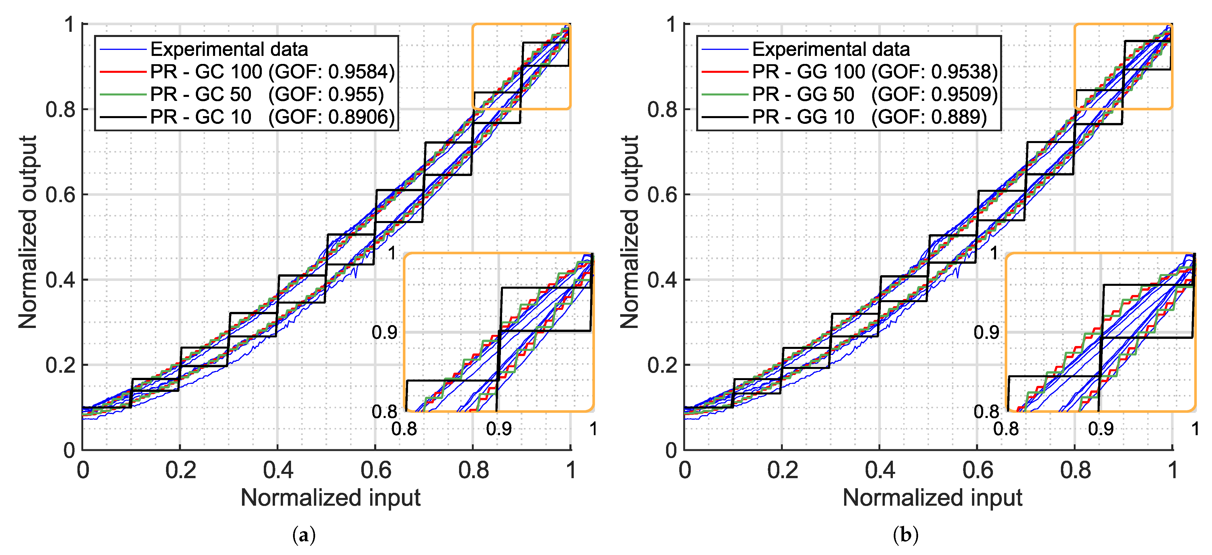
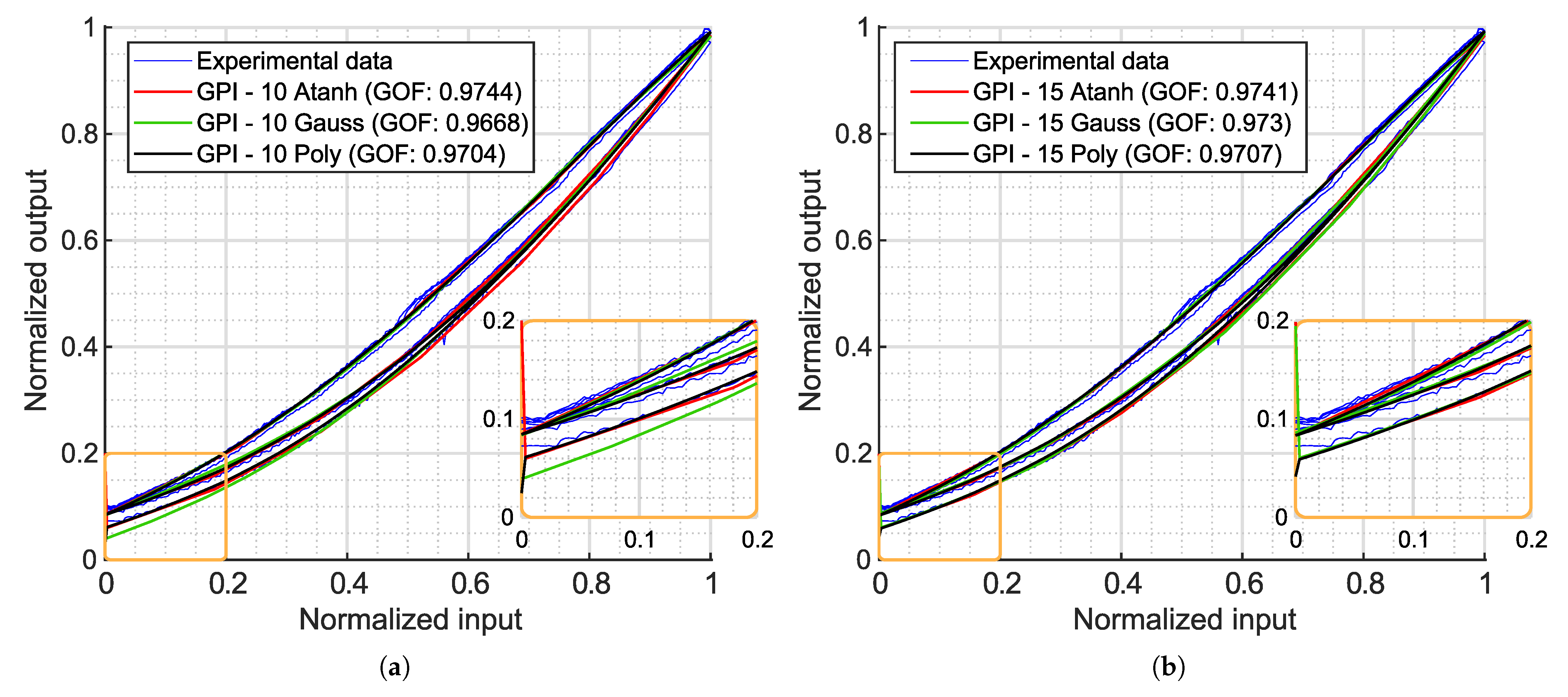
In the first case, 10 operators were selected to capture the general shape of the hysteresis model with a high level of discretization. Increasing the number of operators to 50 allowed for a better continuous approximation of the hysteresis loop, corresponding to a resolution of 0.02 of the normalized input signal. Finally, 100 operators were used to confirm if further increasing the number of operators did not improve the accuracy of the model. In all cases, the GA identified five different parameters: $y_0$, ${\sigma }_{HC}$, ${\mu }_{HC}$, ${\sigma }_{HM}$ and ${\mu }_{HM}$.

Figure 6a shows the fitted PR model using a Gaussian distribution for $p\left(H_M\right)$ and a Cauchy distribution for $p\left(H_C\right)$, while Figure 6b presents the results with Gaussian distributions for both $p\left(H_M\right)$ and $p\left(H_C\right)$. In both cases, the PR model accurately captures the hysteretic behavior of the experimental data. With just 10 operators, the model achieves a GOF close to 0.90, and with 50 operators, it exceeds 0.95. Beyond this point, further increasing the number of operators does not significantly improve the GOF, as the discretization error no longer decreases sufficiently to outweigh the error introduced by the assumed shape of the density functions. In other words, once the discretization is sufficiently fine, the residual error is dominated by the mismatch between the chosen density function and the actual shape of the hysteresis. This effect is more clearly illustrated in the error plots shown in Figure A1 and Figure A2. Therefore, the marginal improvement in the GOF obtained by adding more operators does not sufficiently justify the increased computational cost (see

Table A1. Parameters of fitted Preisach model with 10 operators and Gaussian–Cauchy distributions (GC-10).

Type	${\mathit{\sigma }}_{\mathit{H}\mathit{M}}$	${\mathit{\mu }}_{\mathit{H}\mathit{M}}$	${\mathit{\sigma }}_{\mathit{H}\mathit{C}}$	${\mathit{\mu }}_{\mathit{H}\mathit{C}}$	${\mathit{y}}_0$
Identified	$2.5672$	$6.9125$	$0.0374$	0	$0.9875$
Lower bound	0	0	0	0	0
Upper bound	10	20	1	$0.1$	$0.2$
Simulation time			7 ms

,

Table A2. Parameters of fitted Preisach model with 50 operators and Gaussian–Cauchy distributions (GC-50).

Type	${\mathit{\sigma }}_{\mathit{H}\mathit{M}}$	${\mathit{\mu }}_{\mathit{H}\mathit{M}}$	${\mathit{\sigma }}_{\mathit{H}\mathit{C}}$	${\mathit{\mu }}_{\mathit{H}\mathit{C}}$	${\mathit{y}}_0$
Identified	$3.2352$	$11.6040$	$0.0232$	$0.0001$	$0.0837$
Lower bound	0	0	0	0	0
Upper bound	10	20	1	$0.1$	$0.2$
Simulation time			19 ms

,

Table A3. Parameters of fitted Preisach model with 100 operators and Gaussian–Cauchy distributions (GC-100).

Type	${\mathit{\sigma }}_{\mathit{H}\mathit{M}}$	${\mathit{\mu }}_{\mathit{H}\mathit{M}}$	${\mathit{\sigma }}_{\mathit{H}\mathit{C}}$	${\mathit{\mu }}_{\mathit{H}\mathit{C}}$	${\mathit{y}}_0$
Identified	$3.5237$	$13.8115$	$0.0211$	0	$0.0818$
Lower bound	0	0	0	0	0
Upper bound	10	20	1	$0.1$	$0.2$
Simulation time			48 ms

,

Table A4. Parameters of fitted Preisach model with 10 operators and Gaussian–Gaussian distributions (GG-10).

Type	${\mathit{\sigma }}_{\mathit{H}\mathit{M}}$	${\mathit{\mu }}_{\mathit{H}\mathit{M}}$	${\mathit{\sigma }}_{\mathit{H}\mathit{C}}$	${\mathit{\mu }}_{\mathit{H}\mathit{C}}$	${\mathit{y}}_0$
Identified	$2.7632$	$7.3055$	$0.0586$	0	$0.1001$
Lower bound	0	0	0	0	0
Upper bound	10	20	1	$0.1$	$0.2$
Simulation time			6 ms

,

Table A5. Parameters of fitted Preisach model with 50 operators and Gaussian–Gaussian distributions (GG-50).

Type	${\mathit{\sigma }}_{\mathit{H}\mathit{M}}$	${\mathit{\mu }}_{\mathit{H}\mathit{M}}$	${\mathit{\sigma }}_{\mathit{H}\mathit{C}}$	${\mathit{\mu }}_{\mathit{H}\mathit{C}}$	${\mathit{y}}_0$
Identified	$3.3204$	$11.8789$	$0.0452$	0	$0.0865$
Lower bound	0	0	0	0	0
Upper bound	10	20	1	$0.1$	$0.2$
Simulation time			20 ms

and

Table A6. Parameters of fitted Preisach model with 100 operators and Gaussian–Gaussian distributions (GG-100).

Type	${\mathit{\sigma }}_{\mathit{H}\mathit{M}}$	${\mathit{\mu }}_{\mathit{H}\mathit{M}}$	${\mathit{\sigma }}_{\mathit{H}\mathit{C}}$	${\mathit{\mu }}_{\mathit{H}\mathit{C}}$	${\mathit{y}}_0$
Identified	$3.6125$	$14.1497$	$0.0432$	$0.0002$	$0.0846$
Lower bound	0	0	0	0	0
Upper bound	10	20	1	$0.1$	$0.2$
Simulation time			48 ms

).

The biggest difference between the two fitted combinations is that the Gaussian–Gaussian model slightly separates outward from the measured loop at the upper end (Figure 6b, orange zoom) of the loop. Although this difference is not significant enough to have a major impact on the fitted results (as can be seen comparing the GOF values), the shape change highlights the necessity of finding proper combinations of distribution functions for each particular case.

Finally, the success of the PR model in representing the experimental data is attributed to its ability to capture the asymmetric shape through its density function, which depends on both the upward and downward thresholds. This allows for different paths on each side of the hysteresis loop. The main drawback of this formulation is that the initial loading curve is not modeled. However, it is worth noting that if the loading curve of the experimental data starts in a middle point of the loop and the relay operator takes the value of $-1$ for $x\left(t_k\right)\le \beta$, the PR model should be able to represent loading curves lying within the hysteresis loop.

4. The Prandtl–Ishlinskii Model

The Prandtl–Ishlinskii (PI) model and its variants have become particularly popular in recent years for hysteresis modeling. The reasons for the adoption of PI models include their simplicity and flexibility while allowing for the characterization of saturated and unsaturated hysteretic behaviors [32]. However, perhaps the most important reason is that PI models admit analytical inverses, enabling quick and efficient implementation of feedforward compensators in a wide variety of systems. Multiple examples can be found in the literature, e.g., to compensate for hysteresis in piezoelectric actuators [47,48], magnetostrictive actuators [49] and soft pneumatic actuators [10,50] and to study the ranges of PID controllers [51], adaptive controllers [52], etc.

The PI model exploits two different operators: the play operator and the stop operator, which are introduced in the following sections.

4.1. The Play Operator

The output of the PI play operator ${\Gamma }_r[•]$ with a fixed threshold (also known as the radius) $r\ge 0$, shown in Figure 7, can be defined as follows:

$${\Gamma }_r\left[x\left(t_k\right)\right]=max\{x\left(t_k\right)-r,min\{x\left(t_k\right)+r,{\Gamma }_r\left[x\left(t_{k-1}\right)\right]\}\}$$

(10)

with the initial condition $M_0\in \mathbb{R}$:

$${\Gamma }_r\left[x\left(0\right)\right]=max\{x\left(0\right)-r,min\{x\left(0\right)+r,M_0\}\}$$

(11)

where $t_k=kh,k=1,2,\dots ,K$ represents the time discretization of the input signal under a fixed step size h.

4.2. The Stop Operator

The output of the stop operator ${\Xi }_r[•]$ with a fixed threshold $r\ge 0$ and initial condition $M_0\in \mathbb{R}$, shown in Figure 8, is given by

$${\Xi }_r\left[x\left(t_k\right)\right]=min\{r,max\{-r,x\left(t_k\right)-x\left(t_{k-1}\right)+{\Xi }_r\left[x\left(t_{k-1}\right)\right]\}\}$$

(12)

$${\Xi }_r\left[x\left(0\right)\right]=min\{r,max\{-r,x\left(0\right)+M_0\}\}$$

(13)

4.3. The Classic Prandtl–Ishlinskii Model

The Classic Prandtl–Ishlinskii (CPI) model is based on the weighted superposition of the previously defined operators. However, most of the work related to the CPI model utilizes the formulation based on the play operator [28,32,34,35,36]. In this work, as the measured experimental data moves counterclockwise, only the CPI model using the play operator will be considered. The posterior Maxwell-Slip model section will continue this discussion and further clarify this choice.

With that consideration, the continuous CPI model is given by the expression

$${\Phi }_{PI}\left[x\left(t\right)\right]=p_{0}x\left(t\right)+{\int }_0^{\infty }p\left(r\right){\Gamma }_r\left[x\left(t\right)\right]dr$$

(14)

However, in practical applications, the PI model is constructed by a weighted sum of n play operators ${\Gamma }_{r_i}\left[x\left(t\right)\right]$ (Figure 9):

$${\Phi }_{PI}\left[x\left(t\right)\right]=p_{0}x\left(t\right)+\sum _{i=1}^n{p}_i{\Gamma }_{r_i}\left[x\left(t\right)\right]$$

(15)

where $r_i>0$ are the radius of the different play operators, $p_i\ge 0$ are their weights and $p_0$ is a parameter that represents the non-hysteretic behavior through the linear function $p_{0}x\left(t\right)$.

Fitting Results

In this section, the results obtained from fitting the CPI model with $n=5$ and $n=10$ operators are presented. Using five operators allows the hysteresis loop to be represented with five distinct slopes, which appears to be a reasonable lower bound. Increasing the number to 10 operators effectively doubles the resolution, allowing for an evaluation of how the accuracy improves with more operators.

The CPI formulation (15) does not employ any density function for the weights or distribution for the thresholds. As a result, the optimization algorithm treats them as free parameters, searching for the best possible combination. Specifically, for n play operators, $2·n+2$ different parameters were optimized: $r_i,\cdots ,r_n,p_i,\cdots ,p_n,M_0$ and $p_0$. Consequently, 12 and 22 different parameters were fitted for the 5- and 10-operator models.

Figure 10 shows the results of the fitted CPI models. As observed, even though the GOF of every case exceeds 0.86, results are far from good. In addition, looking at the values of

Table A7. Parameters of fitted CPI model with 5 play operators.

Type	${\mathit{p}}_0$	${\mathit{M}}_0$	${\mathit{r}}_1$	${\mathit{r}}_2$	${\mathit{r}}_3$	${\mathit{r}}_4$
Identified	$0.3223$	$0.1062$	$0.7709$	$0.0455$	$0.9998$	0
Lower bound	0	0	0	0	0	0
Upper bound	1	1	1	1	1	1
Type	$r_5$	$p_1$	$p_2$	$p_3$	$p_4$	$p_5$
Identified	$0.7509$	0	$0.6034$	0	$0.0002$	0
Lower bound	0	0	0	0	0	0
Upper bound	1	3	3	3	3	3
Simulation time				2.3 ms

and

Table A8. Parameters of fitted CPI model with 10 play operators.

Type	${\mathit{p}}_0$	${\mathit{M}}_0$	${\mathit{r}}_1$	${\mathit{r}}_2$	${\mathit{r}}_3$	${\mathit{r}}_4$
Identified	$0.0610$	$0.0862$	$0.8438$	$0.6037$	$0.0314$	$0.0234$
Lower bound	0	0	0	0	0	0
Upper bound	1	1	1	1	1	1
Type	$r_5$	$r_6$	$r_7$	$r_8$	$r_9$	$r_{10}$
Identified	$0.0176$	$0.0215$	$0.0156$	$0.0826$	$0.0805$	$0.0001$
Lower bound	0	0	0	0	0	0
Upper bound	1	1	1	1	1	1
Type	$p_1$	$p_2$	$p_3$	$p_4$	$p_5$	$p_6$
Identified	$0.0006$	$0.0180$	$0.0430$	$0.0035$	$0.0156$	$0.5756$
Lower bound	0	0	0	0	0	0
Upper bound	3	3	3	3	3	3
Type	$p_7$	$p_8$	$p_9$	$p_{10}$
Identified	$0.1777$	$0.6034$	$0.0163$	$0.0156$
Lower bound	0	0	0	0
Upper bound	3	3	3	3
Simulation time				2.5 ms

, it can be deduced that most play operators are not having an important role in the output, highlighting the inability of the model to obtain better results, regardless of the number of operators. This result is also evident from the simulation output and modeling errors shown in Figure A3.

These results can be explained just by examining the structure of the play operator (Figure 7). It can be seen that the upward and downward paths are symmetrical with respect to the center line that connects its maximum value with its minimum, crossing the x axis at a distance $\pm r$ from the origin. Consequently, CPI is a hysteresis model only suited for symmetric hysteresis shapes. To overcome this limitation and address asymmetric hysteresis, an extension known as the Generalized Prandtl–Ishlinskii model has been developed [32].

4.4. The Generalized Prandtl–Ishlinskii Model

The Generalized Prandtl–Ishlinskii (GPI) model is able to represent asymmetric hysteresis (see Figure 11) through the addition of envelope functions to the input signal within the play operator [53]:

$${\Gamma }_r^{\alpha }\left[x\left(t_k\right)\right]=max\{{\alpha }_R\left[x\left(t_k\right)\right]-r,min\{{\alpha }_L\left[x\left(t_k\right)\right]+r,{\Gamma }_r^{\alpha }\left[x\left(t_{k-1}\right)\right]\}\}$$

(16)

with initial condition $M_0\in \mathbb{R}$:

$${\Gamma }_r^{\alpha }\left[x\left(0\right)\right]=max\{{\alpha }_R\left[x\left(0\right)\right]-r,min\{{\alpha }_L\left[x\left(0\right)\right]+r,M_0\}\}$$

(17)

where ${\alpha }_R[•]$ and ${\alpha }_L[•]$ are two odd envelope functions. In addition, for any radius $r\ge 0$, the condition ${\alpha }_R\left[x\left(t\right)\right]+r\ge {\alpha }_L\left[x\left(t\right)\right]-r$ must be satisfied in order to meet the order preservation property of the hysteresis loop [54]. Thus, the discrete output of the GPI model is given by

$${\Phi }_{GPI}\left[x\left(t\right)\right]=G\left[x\left(t\right)\right]+\sum _{i=1}^n{p}_i{\Gamma }_{r_i}^{\alpha }\left[x\left(t\right)\right]$$

(18)

where the non-hysteretic behavior is also generalized by the Lipschitz continuous function $G[•]$. However, it is often considered the same linear relation $p_{0}x\left(t\right)$, which is the assumption made in this work.

From all possible candidates for envelope functions, three types are commonly considered [55]: polynomial functions ${\alpha }_j^{Poly}$, hyperbolic tangent functions ${\alpha }_j^{Tanh}$ and Gaussian functions ${\alpha }_j^{Gauss}$, since they also allow for analytical inverses, preserving one of the key features of the CPI model. They are defined as follows:

$${\alpha }_j^{Poly}\left[x\left(t\right)\right]=x{\left(t\right)}^2+a_{j}x\left(t\right)+b_j$$

(19)

$${\alpha }_j^{Tanh}\left[x\left(t\right)\right]=a_{j}tanh(x\left(t\right)+b_j)+c_j$$

(20)

$${\alpha }_j^{Gauss}\left[x\left(t\right)\right]=a_j{e}^{-{\displaystyle \frac{{(x\left(t\right)-b_j)}^2}{2c_j}}}$$

(21)

where $a_j,b_j,c_j\in \mathbb{R}$ are the parameters of the considered functions and $j=R$ or L represent the upward or downward envelope functions ${\alpha }_R$ and ${\alpha }_L$.

Consequently, in this work, to reduce the number of parameters to be identified, one can consider n equally spaced values for $r_i$ between $min\left(x\right(t\left)\right)$ and $max\left(x\right(t\left)\right)$ and propose a proper vanishing density function, such as

$$p_i={\delta }_1{e}^{-{\delta }_2{r}_i}$$

(22)

where ${\delta }_1,{\delta }_2\ge 0$ are adjustable parameters.

Fitting Results

The results of fitting the GPI model are presented in this section. With the formulation presented in Equations (18)–(22), the number of parameters does not increase with the number of operators, as was the case with the CPI model. Arbitrarily, we chose 10 and 15 operators to check whether the number of operators affects the accuracy of the model.

A total of eight different parameters were adjusted for the GPI model with polynomial functions using the GA: $p_0,M_0,{\delta }_1,{\delta }_2,a_R,a_L,b_R$ and $b_L$. For the GPI model with hyperbolic tangent and Gaussian functions, two additional parameters were also calculated: $c_R$ and $c_L$.

Figure 12a,b show the results of fitting the GPI with the three previously described envelope functions for $n=10$ and $n=15$ equally spaced operators, respectively. It can be seen that in all cases, the GPI model is capable of accurately capturing the asymmetric behavior of the experimental data, regardless of the envelope functions or the number of operators, achieving more than 0.97 as GOF.

Moreover, and as an important difference to that of the Preisach model, all configurations follow the initial loading curve. The only exception was observed with the Gaussian functions using 10 operators, where GOF slightly fell below 0.97. As shown in the zoomed section of Figure 12a, this discrepancy is mainly due to difficulties representing the first instants of the loading curve.

Another aspect worth mentioning is the computation time. As summarized in

Table A9. Parameters of fitted GPI model with 10 play operators and hyperbolic tangent functions as envelopes.

Type	${\mathit{p}}_0$	${\mathit{M}}_0$	${\mathit{\delta }}_1$	${\mathit{\delta }}_2$	${\mathit{a}}_{\mathit{R}}$
Identified	$0.4084$	$0.1185$	$0.1872$	$0.1920$	$1.2251$
Lower bound	0	0	0	0	$-5$
Upper bound	2	$0.2$	3	3	5
Type	$b_R$	$c_R$	$a_L$	$b_L$	$c_L$
Identified	$-0.5371$	$0.2911$	$2.1285$	$-1.9745$	$1.7202$
Lower bound	$-5$	$-5$	$-5$	$-5$	$-5$
Upper bound	5	5	5	5	5
Simulation time			6 ms

,

Table A10. Parameters of fitted GPI model with 10 play operators and Gaussian functions as envelopes.

Type	${\mathit{p}}_0$	${\mathit{M}}_0$	${\mathit{\delta }}_1$	${\mathit{\delta }}_2$	${\mathit{a}}_{\mathit{R}}$
Identified	$0.4340$	$0.1997$	$0.0731$	$2.9961$	$4.9515$
Lower bound	0	0	0	0	$-5$
Upper bound	2	$0.2$	3	3	5
Type	$b_R$	$c_R$	$a_L$	$b_L$	$c_L$
Identified	$1.6332$	$2.3430$	$2.8279$	$1.2269$	$4.6150$
Lower bound	$-5$	$-5$	$-5$	$-5$	$-5$
Upper bound	5	5	5	5	5
Simulation time			5 ms

,

Table A11. Parameters of fitted GPI model with 10 play operators and polynomial functions as envelopes.

Type	${\mathit{p}}_0$	${\mathit{M}}_0$	${\mathit{\delta }}_1$	${\mathit{\delta }}_2$
Identified	$0.1060$	$0.0485$	$0.1752$	$2.7863$
Lower bound	0	0	0	0
Upper bound	2	$0.2$	3	3
Type	$a_R$	$b_R$	$a_L$	$b_L$
Identified	$0.7144$	$0.3616$	$0.8169$	$-0.4579$
Lower bound	$-5$	$-5$	$-5$	$-5$
Upper bound	5	5	5	5
Simulation time			4 ms

,

Table A12. Parameters of fitted GPI model with 15 play operators and hyperbolic tangent functions as envelopes.

Type	${\mathit{p}}_0$	${\mathit{M}}_0$	${\mathit{\delta }}_1$	${\mathit{\delta }}_2$	${\mathit{a}}_{\mathit{R}}$
Identified	$0.4112$	$0.1168$	$0.1392$	$0.3965$	$1.1818$
Lower bound	0	0	0	0	$-5$
Upper bound	2	$0.2$	3	3	5
Type	$b_R$	$c_R$	$a_L$	$b_L$	$c_L$
Identified	$-0.5628$	$0.2930$	$3.0660$	$-2.1665$	$2.6897$
Lower bound	$-5$	$-5$	$-5$	$-5$	$-5$
Upper bound	5	5	5	5	5
Simulation time			8 ms

,

Table A13. Parameters of fitted GPI model with 15 play operators and Gaussian functions as envelopes.

Type	${\mathit{p}}_0$	${\mathit{M}}_0$	${\mathit{\delta }}_1$	${\mathit{\delta }}_2$	${\mathit{a}}_{\mathit{R}}$
Identified	$0.0211$	$0.0402$	$0.5272$	$0.9960$	$0.7821$
Lower bound	0	0	0	0	$-5$
Upper bound	2	$0.2$	3	3	5
Type	$b_R$	$c_R$	$a_L$	$b_L$	$c_L$
Identified	$1.7173$	$1.2988$	$-0.3348$	$-0.0557$	$2.1765$
Lower bound	$-5$	$-5$	$-5$	$-5$	$-5$
Upper bound	5	5	5	5	5
Simulation time			6 ms

and

Table A14. Parameters of fitted GPI model with 15 play operators and polynomial functions as envelopes.

Type	${\mathit{p}}_0$	${\mathit{M}}_0$	${\mathit{\delta }}_1$	${\mathit{\delta }}_2$
Identified	$0.1751$	$0.0813$	$0.1199$	$2.9982$
Lower bound	0	0	0	0
Upper bound	2	$0.2$	3	3
Type	$a_R$	$b_R$	$a_L$	$b_L$
Identified	$0.5957$	$0.3082$	$0.6642$	$-0.3798$
Lower bound	$-5$	$-5$	$-5$	$-5$
Upper bound	5	5	5	5
Simulation time			5 ms

, the simulation time of the GPI model for the input signal is between 4 and 8 ms, comparable to the Preisach model with 10 operators (Table A1) but faster than the nearly 20 ms needed for the Preisach model with 50 operators, while consistently yielding better GOF values.

The only minor drawback observed during the GPI model fitting is that simulated initial values deviate from the real initial value of the experimental data. For instance, in Figure 12a the hyperbolic tangent fit has an initial value of around 0.2, while in Figure 12b this effect is observed for the Gaussian fit. This discrepancy is also evident in Figure A4 and Figure A5. Nevertheless, this issue has a simple treatment, even in control loops, since it only affects the first point of the model.

5. The Maxwell-Slip Model

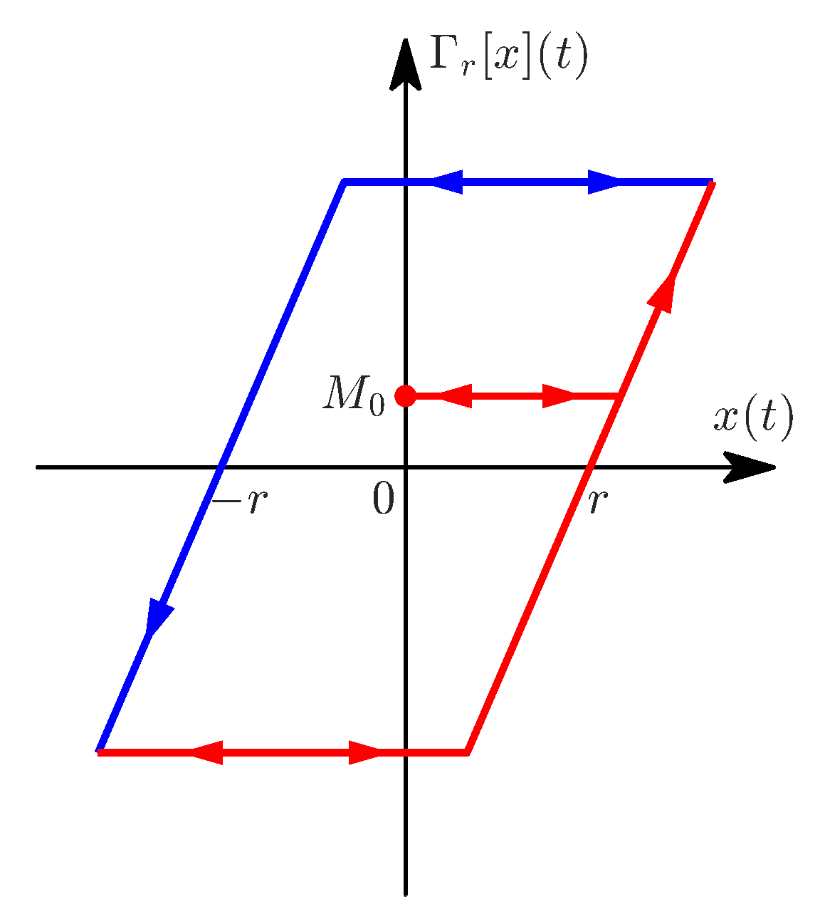
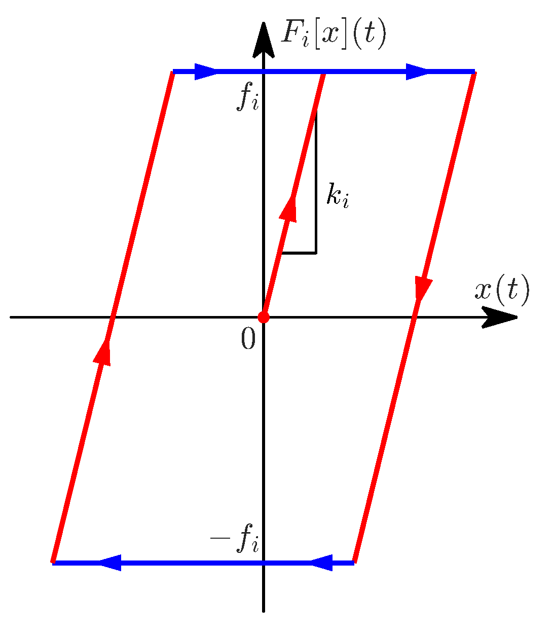
The Maxwell-Slip model (MS) is a hysteresis model originally proposed to describe the behavior of friction in mechanical systems. Nowadays, due to its simplicity and facility of computation, it has been used to model hysteresis in a wide range of actuators [56,57,58,59]. The MS model is based on the elasto-slide operator $F_i[•]$, shown in Figure 13:

$$F_i\left[x\left(t\right)\right]=\left\{\begin{array}{cc}{k}_i(x\left(t\right)-x_{b_i}),\hfill & \mathrm{if}\left|k_i(x\left(t\right)-x_{b_i})\right|<f_i\hfill \\ f_i·\mathrm{sgn}\left(\dot{x}\left(t\right)\right)\mathrm{and}{x}_{b_i}=x\left(t\right)-{\displaystyle \frac{f_i}{k_i}}·\mathrm{sgn}\left(\dot{x}\left(t\right)\right),\hfill & \mathrm{otherwise}\hfill \end{array}\right.$$

(23)

Here, $\dot{x}\left(t\right)$ denotes the time derivative of $x\left(t\right)$. The elasto-slide operator is normally represented as a massless linear spring in combination with a massless block subject to Coulomb friction, where $k_i$ is the stiffness of each spring, $f_i={\mu }_i·N_i$ is the breakaway friction force and $x_{b_i}$ is position of each block. In addition, $\mathrm{sgn}(•)$ is the sign function defined as

$$\mathrm{sgn}\left(\dot{x}\left(t\right)\right)=\left\{\begin{array}{cc}1,\hfill & \mathrm{for}\dot{x}\left(t\right)>0\hfill \\ 0,\hfill & \mathrm{for}\dot{x}\left(t\right)=0\hfill \\ -1,\hfill & \mathrm{for}\dot{x}\left(t\right)<0\hfill \end{array}\right.$$

(24)

Sometimes, the elasto-slide operator is interpreted as an elasto-plastic operator that acts elastically until the force threshold $f_i$ is surpassed, where the plastic behavior takes control. This plastic or sliding behavior is responsible for capturing the memory effects of the hysteresis. The output of the MS model is the summation of multiple parallel elasto-slide elements (Figure 14) with an initial value $w_0$:

$${\Phi }_{MS}\left(x\left(t\right)\right)=w_0+\sum _{i=1}^n{F}_i$$

(25)

It is worth noting that the shape of the elasto-slide operator is similar to that of the stop operator in the PI model (Figure 8). Consequently, the results obtained with this model would be similar to those of the stop operator-based CPI model.

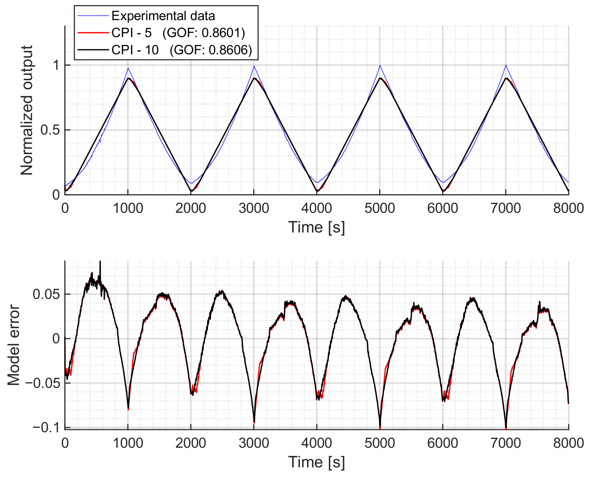
Fitting Results

The fitted MS model with $n=10$ operators is presented in this section. As will be explained later, the number of operators does not affect the outcome. Similar to the CPI model, the threshold and stiffness coefficients were treated as free parameters, without any constraining functions. Thus, $2·n+1$ different parameters were identified: $w_0$, $f_1,\cdots ,f_n$ and $k_1,\cdots ,k_n$.

The results of the fitted MS model can be found in Figure 15. As shown in the figure, the obtained model represents a straight line, failing to capture the nonlinear dynamics of the measured data. This behavior is also clearly observable in the upper plot (the simulation output) of Figure A6.

Regardless of the number of operators, the results will remain the same. This is because the behavior of the fitted model is effectively reproduced by fitting the slope k of a single elasto-slide operator, ensuring that, over the input signal range, it never reaches the breakaway friction force f. This limitation arises because the elasto-slide operator represents loops that move clockwise, while the experimental data moves counterclockwise. Thus, this formulation of the MS model is not suitable for modeling the hysteretic behavior of the proposed soft pneumatic actuator.

6. The Bouc–Wen Model

The Bouc–Wen model (BW) is a hysteresis model based on differential equations that has been widely used to describe hysteretic behavior in civil and structural systems. It is highly valued for its capability of capturing, in an analytical form, a wide range of shapes. Usually, BW formulates the relationship between displacement and restoring force, and its most famous variations, e.g., the Bouc–Wen–Baber–Noori model [60,61], include other commonly structural phenomenons such as pitching, stiffness and strength degradation. However, as previous analyzed models, its abstract mathematical structure makes the BW model suitable for several types of systems. In addition, since it is based on differential equations, the BW model has become very popular in compensation control approaches, for example, in adaptive controllers for piezoelectric actuators [62,63] and structural systems [64], the tuning of PID controllers [24], etc.

6.1. The Classical Bouc–Wen Model

The Classical Bouc–Wen model (CBW) represents hysteretic behavior through a nonlinear differential Equation (26):

$$\dot{z}\left(t\right)=D^{-1}(A\dot{x}\left(t\right)-\beta \left|\dot{x}\left(t\right)\right|{\left|z\left(t\right)\right|}^{n-1}z\left(t\right)-\gamma \dot{x}\left(t\right){\left|z\left(t\right)\right|}^n)$$

(26)

$${\Phi }_{BW}\left[x\left(t\right)\right]=\alpha \kappa x\left(t\right)+(1-\alpha )D\kappa z\left(t\right)$$

(27)

where $z\left(t\right)$ represents the hysteretic behavior and $n\ge 1$, $D>0$, $A,\beta ,\gamma \in \mathbb{R}$ are the parameters that control the hysteresis shape, subject to $\beta +\gamma \ne 0$. In addition, the nonlinear equation of the CBW model is usually cascaded with equation (27), where the parameter $0\le \alpha \le 1$ is used to tune the relationship between the linear and the nonlinear hysteretic behavior and $\kappa >0$ is a parameter to control the scaling of the output.

Fitting Results

In this section, the results of fitting the CBW model (26), (27) are presented. In this case, the optimization algorithm fitted eight different parameters: $\alpha ,\kappa ,D,A,\beta ,\gamma ,n$ and $z\left(0\right)$, which serves as the initial condition for the ODE solver.

The fitted CBW model can be seen in Figure 16. As observed, the CBW fitting fails to represent the asymmetric behavior of the experimental data. Indeed, as it is widely established in the literature [24,29], the CBW is only valid for symmetric hysteresis. In addition, the resulting behavior closely resembles that obtained with the CPI model (see Figure 10, Figure A3 and Figure A7). Therefore, it can be interpreted that the CBW provides the best continuous approximation that can be achieved without accounting for the asymmetric behavior of the experimental data. Fortunately, several extensions of the CBW model that are capable of representing asymmetric hysteresis loops have been developed.

Also, it is worth noting that the CBW model is known for its high sensitivity to parameter tuning, often requiring several iterations to achieve convergence. However, in this work, that was not the case, as all three iterations yielded similar results.

6.2. Asymmetric Bouc–Wen Models

To model asymmetrical hysteresis, a function to represent asymmetry $\psi \left[x\right(t\left)\right]$ is introduced into the Bouc–Wen model (Equation (28)), obtaining the Asymmetric Bouc–Wen model (ABW):

$$\dot{z}\left(t\right)=D^{-1}(A\dot{x}\left(t\right)-\beta \left|\dot{x}\left(t\right)\right|{\left|z\left(t\right)\right|}^{n-1}z\left(t\right)-\gamma \dot{x}\left(t\right){\left|z\left(t\right)\right|}^n+\psi \left[x\left(t\right)\right])$$

(28)

$${\Phi }_{BW}\left[x\left(t\right)\right]=\alpha \kappa x\left(t\right)+(1-\alpha )D\kappa z\left(t\right)$$

(29)

The function takes different forms depending on the work. For example, in [65,66], the function $\psi \left[x\right(t\left)\right]$ has the form

$$\psi \left[x\left(t\right)\right]=\delta x\left(t\right)\mathrm{sgn}\left(\dot{x}\left(t\right)\right)$$

(30)

where $\delta \in \mathbb{R}$ is the non-symmetric correction factor.

Figure 17a shows the shape of this equation to different values of $\delta$. As is shown, the asymmetric function (30) moves in a linear shape until $x\left(t\right)$ stops increasing, where the function jumps to negative values. Thus, this function increases the difference between upward and downward paths in the upper right corner of the hysteresis loop, where $x\left(t\right)$ is maximum.

More complex behaviors can be obtained if additional functions are included. For example, in [67], $\psi \left[x\right(t\left)\right]$ is defined using a sigmoid function jointly with the sign function to obtain a more pronounced asymmetric behavior:

$$\psi \left[x\left(t\right)\right]=\delta [1+\mathrm{sgn}\left(\dot{x}\left(t\right)\right)]\left({\displaystyle \frac{1}{1+e^{-p\left(x\right(t)-q)}}}-{\displaystyle \frac{1}{2}}\right)$$

(31)

where $p\ge 0$ determines the rate of convergence of the sigmoid function and $q\in [min(x\left(t\right)),max(x\left(t\right)\left)\right]$ determines if the correction term is convex, concave or a combination of both.

Figure 17b shows the shape of Equation (31), which has the behavior of the defined sigmoid function when $\mathrm{sgn}\left(\dot{x}\left(t\right)\right)=1$ and jumps to a horizontal line at zero when $\mathrm{sgn}\left(\dot{x}\left(t\right)\right)=-1$, i.e., this function only works when $x\left(t\right)$ moves upward, adding in that way the asymmetric behavior.

Fitting Results

The fitted ABW models are presented in this section. The ABW model with Equation (30) (hereafter referred to as ${\mathrm{ABW}}_1$) includes one additional parameter compared with the CBW model (the parameter $\delta$). Therefore, a total of nine parameters were required to model the asymmetric hysteresis loop. In the case of Equation (31) (hereafter referred to as ${\mathrm{ABW}}_2$), two additional parameters were required (parameters p and q), bringing the total number of parameters to 11.

The results of fitting the ${\mathrm{ABW}}_1$ are presented in Figure 18a. It can be seen that using this function significantly increases the GOF compared with the CBW, reaching values above 0.93 and successfully representing the asymmetric behavior (the errors associated with this model are shown in Figure A8).

However, a closer inspection (see zoomed-in view within Figure 18a) reveals that this model is not consistent with the physical behavior observed in the experimental data. Specifically, the increasing and decreasing paths crossed before reaching their maximum values. As it was explained before, function (30) increases the difference between upward and downward paths when $x\left(t\right)$ is maximum. As the upper end of the experimental data is pointed, the optimization algorithm tries to compensate for this difference with the model values, forcing the apparition of an artificial loop. Therefore, despite the high GOF, this model cannot be accepted (as valid) to model our experimental data.

On the other hand, the ${\mathrm{ABW}}_2$ model, shown in Figure 18b, represents a physically consistent hysteresis loop, with a GOF higher than 0.96. In addition, this model accurately reproduces the loading curve —clearly visible in Figure A9— modeling all the key features of the experimental data with a simulation time of only 3 ms.

7. Comparative Analysis and Conclusions

This section presents a comparative analysis of the models fitted to the experimental data.

Table 1. A summary of the fitting results for each phenomenological model.

Type	GOF	SimulationTime [ms]	Numberof Parameters	Key Fitting Results
PR-GC (10 operators)	$0.8906$	7	5	✓ Captures asymmetric behavior ✗ Unable to capture loading curve ✗ With a low discretization level and high computation time
PR-GG (10 operators)	$0.889$	6	5
PR-GC (50 operators)	$0.955$	19	5
PR-GG (50 operators)	$0.9509$	20	5
PR-GC (100 operators)	$0.9584$	48	5
PR-GG (100 operators)	$0.9538$	48	5
CPI (5 operators)	$0.8601$	$2.3$	12	✗ Unable to capture asymmetric behavior
CPI (10 operators)	$0.8606$	$2.5$	22
GPI-Atanh (10 operators)	$0.9744$	6	10	✓ Captures asymmetric behavior ✓ Captures loading curve ✓ Best balance between fidelity, complexity and computational efficiency ✗ Initial point may differ from the real initial value
GPI-Atanh (15 operators)	$0.9741$	8	10
GPI-Gauss (10 operators)	$0.9668$	5	10
GPI-Gauss (15 operators)	$0.973$	6	10
GPI-Poly (10 operators)	$0.9704$	4	8
GPI-Poly (15 operators)	$0.9707$	5	8
MS (10 operators)	$0.8293$	$2.5$	21	✗ Unable to represent the experimental loop: clockwise operator ✗ Unable to capture asymmetric behavior
CBW	$0.8614$	3	8	✗ Unable to capture asymmetric behavior
${\mathrm{ABW}}_1$	$0.9367$	4	9	✓ Captures asymmetric behavior ✓ With appropriate functions, captures loading curve (${\mathrm{ABW}}_2$) ✗ Without appropriate functions, produces inconsistent behavior (${\mathrm{ABW}}_1$)
${\mathrm{ABW}}_2$	$0.9634$	3	11

summarizes the GOF values, simulation times and number of adjusted parameters for each model, along with a brief overview of the key results for each formulation.

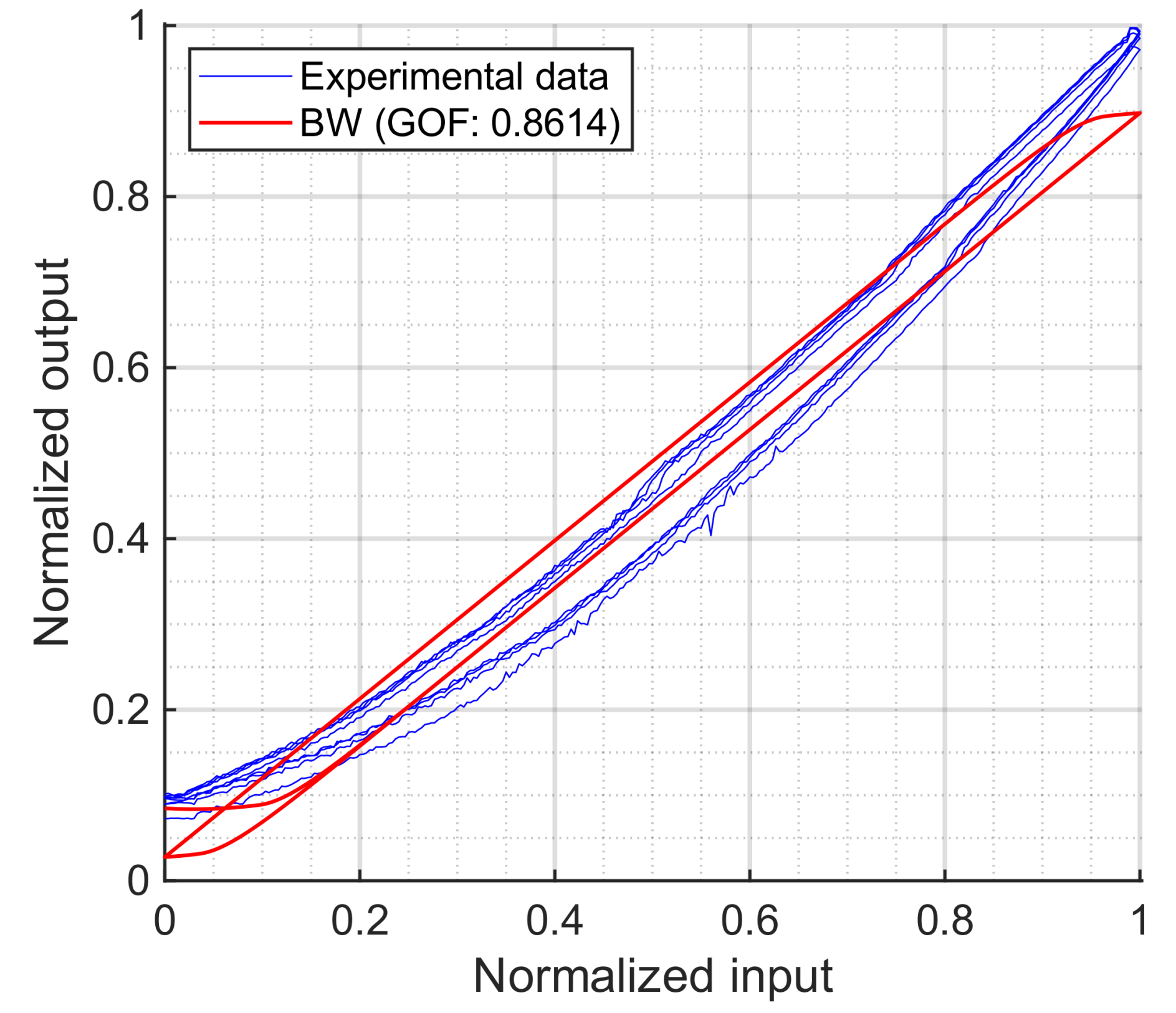
The first conclusion is that the CPI and CBW models are discarded, as they fail to capture the asymmetric behavior of the actuator. The MS model (also unable to represent asymmetry) performs the worst with our experimental data. As discussed in its corresponding results section, the elasto-slide operator produces loops in the opposite direction to those observed experimentally. These shortcomings highlight the importance of selecting models and operators that align with the shape and direction of the experimental loop.

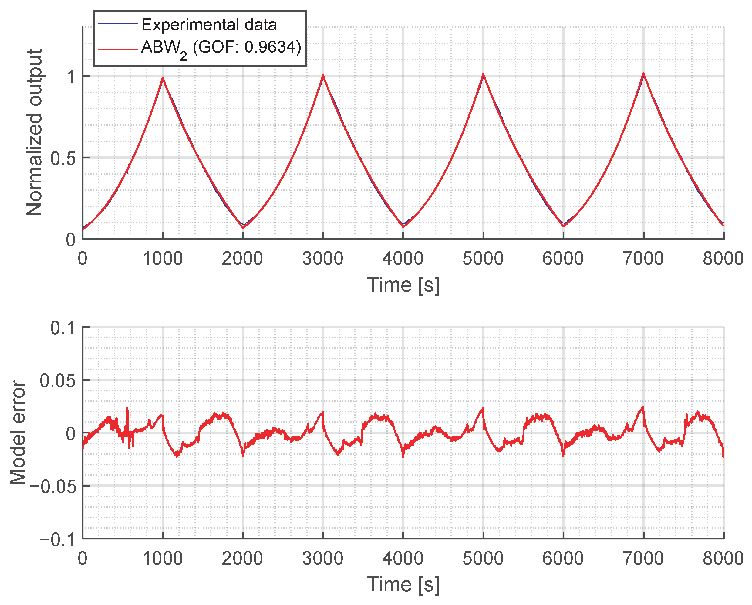
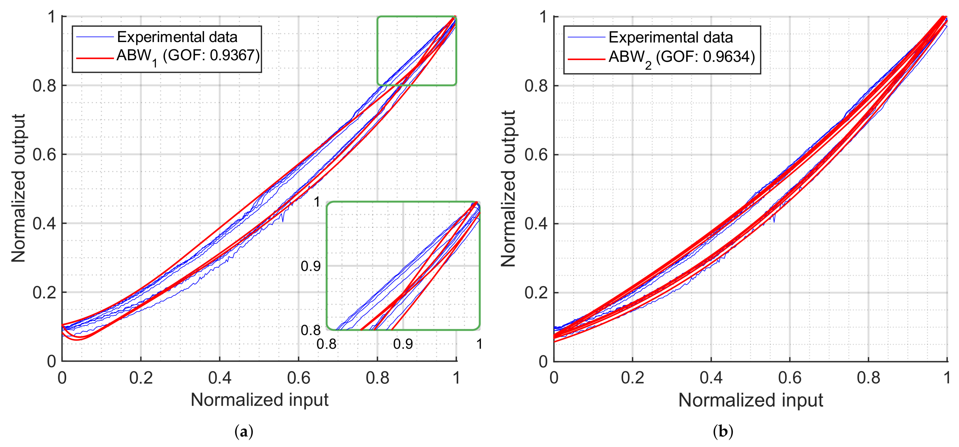
Among the asymmetric models analyzed, all achieved good fits, but the ABW is the most questionable: depending on the chosen asymmetry functions, it can produce hysteresis loops that are not physically consistent with the experimental data, as with the case of Equation (30). However, with appropriately selected functions, it can yield continuous and feasible representations of all the key features of the hysteresis loop (i.e., the loading curve, the asymmetric shape, etc.), as demonstrated by the formulation shown in Equation (31).

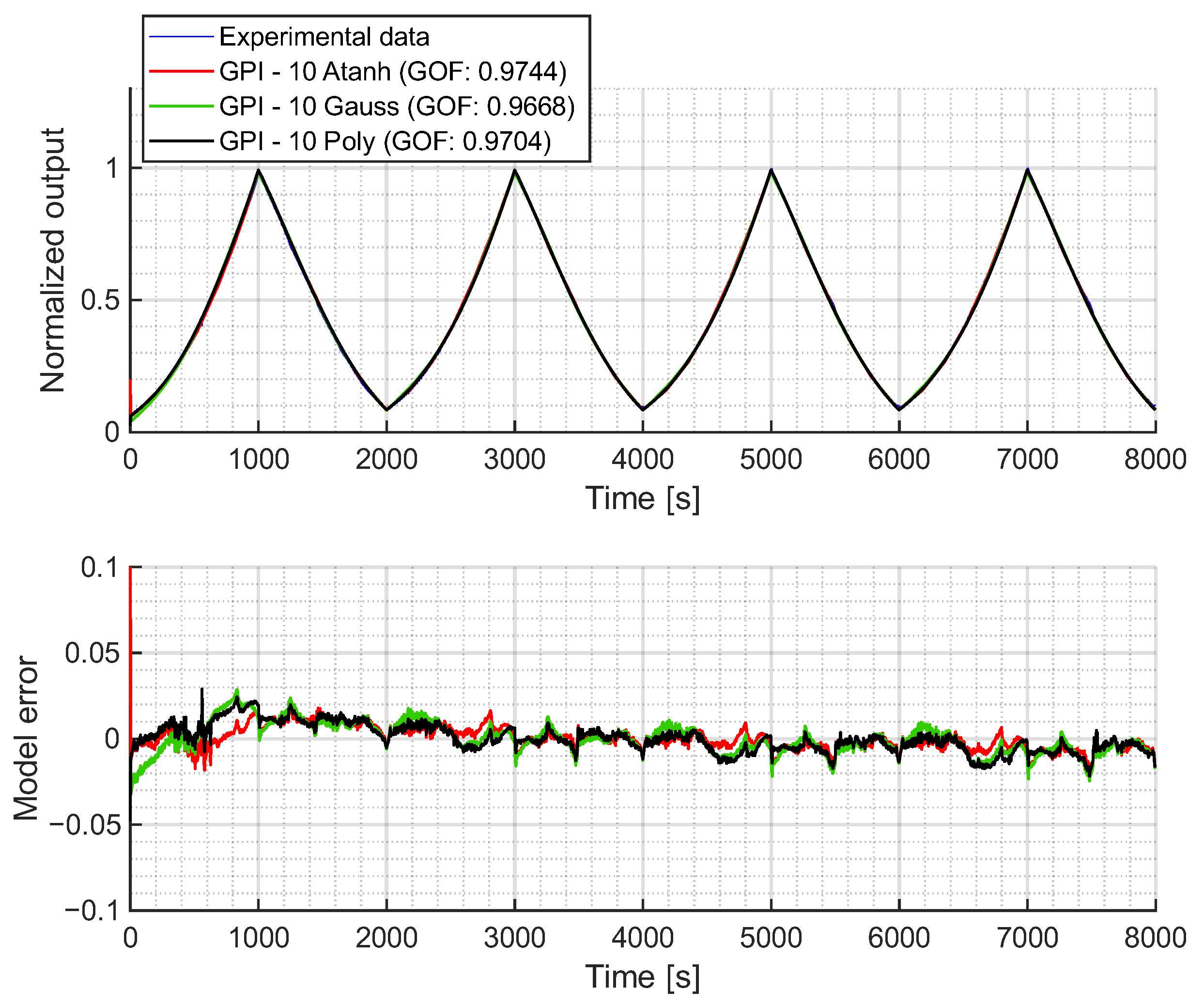
The PR model has the advantage of requiring the fewest parameters. With only five parameters, it successfully captures the asymmetry of the hysteresis loop. Nevertheless, it has two main limitations. First, the presented formulation does not reproduce the loading curve, although, as discussed in its section, alternative formulations may overcome this. Second, at least 50 operators are required to represent the hysteresis loop with low discretization, resulting in a longer computation time compared to the other models. This is the only model which exceeds the 10 ms barrier, which may be critical in some real-time control loops. Reducing the number of operators could shorten computation time but would increase discretization error, which may be problematic in precision applications.

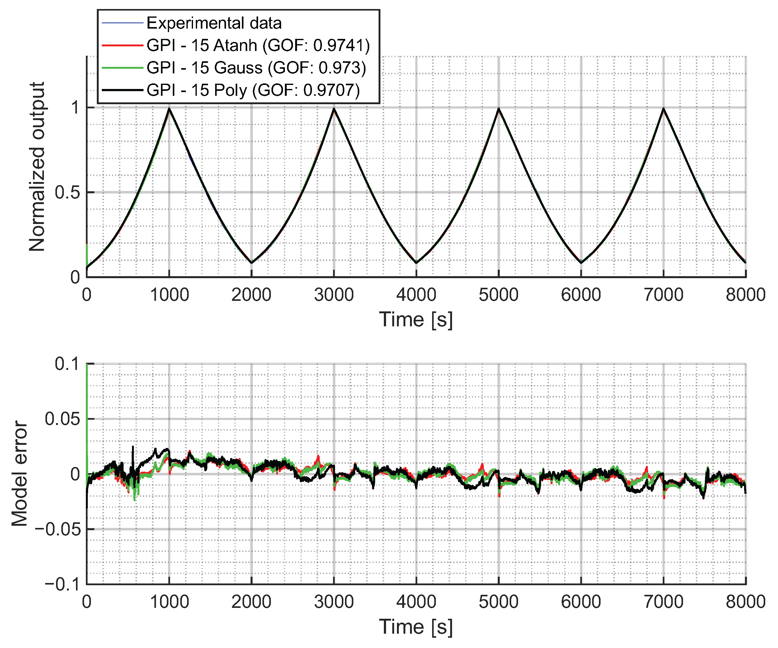
In any case, balancing accuracy, physical consistency, complexity and computational efficiency, the GPI model is likely the best choice for these soft pneumatic actuators. Even with 10 operators, it achieves a GOF above 0.96 in every case. Its explicit mapping, analytical invertibility and high GOF make it particularly well suited for both characterization and feedforward control implementation in applications requiring precise, real-time hysteresis compensation. Its only minor drawback is that the estimated initial value deviates from that of the experimental data. However, this can be easily corrected even in control loops. Within the envelope functions tested, the hyperbolic tangent achieves the highest GOF. However, the use of polynomial envelope functions is likely the best option: they capture the hysteretic behavior accounting for all the key dynamical properties of the system, with minimal loss in accuracy (approximately 0.974 with hyperbolic tangent vs. 0.97 with polynomial envelope functions) and reducing the number of parameters from 10 to 8.

8. Discussion

This work presents a direct comparative evaluation of different phenomenological hysteresis models, applying them to experimental data obtained from a hydrogel-based pneumatic bending actuator. The key concepts of each model are examined, highlighting the trade-offs between modeling fidelity, physical consistency, computational cost and implementation. Operator-based models, such as PR, CPI, GPI and MS, have been compared, emphasizing the importance of a careful selection of operators and the implementation of appropriate density functions.

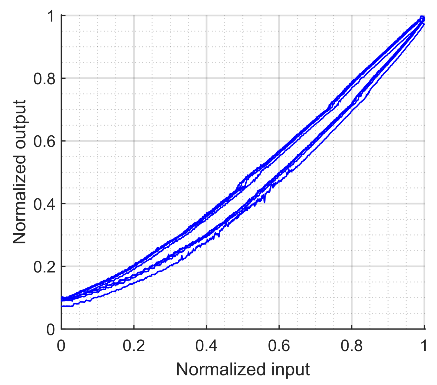
Moreover, the pronounced asymmetrical behavior in the experimental data underlines the necessity of using asymmetric hysteresis models, such as PR, GPI or ABW models. As shown in the section on the ABW model (Section 6.2), careful attention must be paid to model implementation, since not all asymmetric formulations yield feasible or accurate solutions.

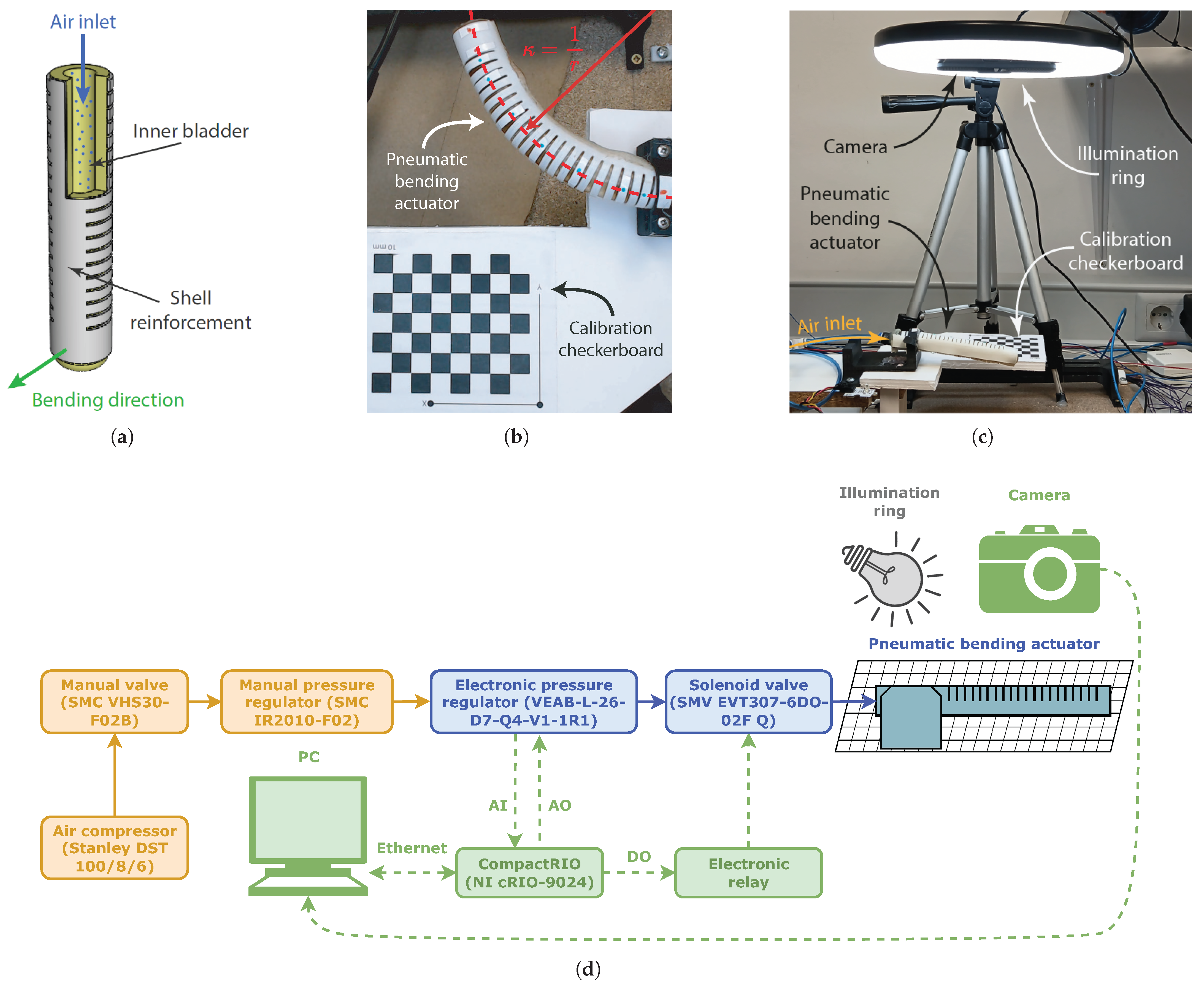
The experimental procedure has been designed to isolate the pure hysteretic behavior of the actuator using low-frequency (0.05 Hz) triangular input signals, effectively decoupling it from other dynamic effects. This analysis, however, was not designed to assess how the models perform under more dynamic operating conditions (e.g., rapid actuation or complex multi-frequency inputs), where viscoelastic and pneumatic dynamics may interact more strongly. Also, all experiments were conducted using a single amplitude (2 V) input signal, without exploring variations in actuation range. As a result, the formation and modeling of minor hysteresis loops have not been studied.

Future work can be built on these limitations by incorporating amplitude and frequency sweeps to evaluate model performance across a broader operational space. Doing so would enable a more complete understanding of hysteresis, using the present results as a reference for the static hysteretic behavior of the actuator and allowing for a clearer decoupling between hysteresis and other phenomena.

Undoubtedly, accurate modeling of actuator hysteresis can inform decisions during the design process, allowing for the development of soft actuators that exhibit reduced hysteresis based on their structural configuration or the materials used. Moreover, precise modeling can support the design of control strategies, as discussed in this work. This aligns with existing research, where various control strategies have been proposed to compensate for hysteresis effects and thereby enhance the tracking and positioning performance of smart actuators. These approaches underscore the necessity of advanced control methodologies to overcome the inherent nonlinearities of soft actuators, thereby ensuring reliable performance in sensitive and dynamic environments.

Therefore, the analysis and insights presented in this work aim to offer a clear guidance for researchers and engineers in the hysteresis modeling of actuators.