Article

Magnetic Field Analytical Calculation of No-Load Electromagnetic Performance of Line-Start Explosion-Proof Permanent Magnet Synchronous Motors Considering Saturation Effect

by
Jinhui Liu
1,2,3,4,
Yunbo Shi
2,
Yang Zheng
1,3,5 and
Minghui Wang
1,3,*
1
School of Electrical and Electronic Engineering, Harbin University of Science and Technology, Harbin 150080, China
2
Instrument Science and Technology Postdoctoral Research Station, Harbin University of Science and Technology, Harbin 150080, China
3
National Engineering Research Center of Large Electric Machines and Heat Transfer Technique, Harbin University of Science and Technology, Harbin 150080, China
4
Shandong Lijiu Electrical Machinery Co., Ltd., Rushan 264500, China
5
Ulanqab Power Supply Branch of Inner Mongolia Electric Power (GROUP) Co., Ltd., Ulanqab 012000, China
*
Author to whom correspondence should be addressed.
Actuators 2025, 14(6), 294; https://doi.org/10.3390/act14060294
Submission received: 17 May 2025 / Revised: 13 June 2025 / Accepted: 16 June 2025 / Published: 17 June 2025
(This article belongs to the Section Actuators for Manufacturing Systems)

Abstract

:
This paper proposes an improved analytical model for a line-start explosion-proof magnet synchronous motor that considers the effect of magnetic bridge saturation. Under the condition of maintaining the air-gap magnetic field unchanged, and taking into account the topological structures of embedded magnets, squirrel cages, and rotor slot openings, a subdomain model partitioning method is systematically investigated. Considering the saturation effect of the magnetic bridge of the rotor, the equivalent magnetic circuit method was utilized to calculate the permeance of the saturated region. It not only facilitates the establishment of subdomain equations and corresponding subdomain boundary conditions, but also ensures the maximum accuracy of the equivalence by maintaining the topology of the rotor. The motor was partitioned into subdomains, and in conjunction with the boundary conditions, the Poisson equation and Laplace equation are solved to obtain the electromagnetic performance of the motor. The accuracy of the analytical model is verified through finite element analysis. The accuracy of the analytical model is verified through finite element analysis (FEA). Compared to the FEA, the improved model maintains high precision while reducing computational time and exhibiting better generality, making it suitable for the initial design and optimization of industrial motors.

1. Introduction

Line-start permanent magnet synchronous motors (LSPMSMs) are characterized by their compact design, high power density, reliable operation and easy starting, making them suitable for a wide range of industrial applications, such as mining and construction [1]. The LSPMSM generates torque through the squirrel cage of the motor’s own structure during the asynchronous state to realize the direct starting of the motor, and its working principle is basically the same as that of the magnet synchronous motor during the steady state operation [2,3,4,5]. The electromagnetic field calculation of the motor is the basis for analyzing the performance of the motor, and it is an important index to measure whether the motor meets the design requirements. A fast and accurate solution of the electromagnetic performance of the motor helps to improve the design efficiency and the design level of the motor, which is of great significance for practical engineering.
Currently, most researchers use finite element analysis (FEA) to solve the electromagnetic properties of motors, such as air-gap flux density, back electromotive force (EMF) and loss, etc. FEA, as a popular solution method, has high computational accuracy and better adaptability. For the fault diagnosis [6], analytical method validation [7], design [8] and development of motors, the finite element method can accurately obtain the electromagnetic performance of the motor through a large number of meshes. However, in the design of motors, FEA computation increases mesh count, demands greater computer performance, and consumes significant time when dealing with intricate structures, large volumes, and frequent structural modifications. Therefore, the selection of an appropriate solution method is crucial for the electromagnetic performance analysis of motors.
The analytical methods for the magnetic field of magnet synchronous motors include the subdomain method based on the Poisson equation, the equivalent magnetic circuit method combining the magnetic network method and the magnetic circuit method, and the analytical method based on the winding function. The equivalent magnetic circuit method is generally used to treat nonlinear problems, such as solving the permeance of the saturated region of the magnetic bridge of a magnet synchronous motor [9]. In Refs. [10,11,12], a novel three-dimensional magnetic network model was developed to optimize and predict the magnetic field of a motor. However, the accuracy of the equivalent magnetic network method solution depends on the number of network nodes and the mesh shape. Moreover, the equivalent magnetic network method can only obtain the average magnetic field, and the accuracy for the electromagnetic force analysis of the motor cannot be guaranteed [13]. The air-gap flux density and self-inductance of the excitation winding are analyzed based on the improved winding function method, but the analytical accuracy of the winding function method is not guaranteed for some motors due to the irregular topology of the motor [14].
In the analytical solution of the motor magnetic field, the subdomain method can accurately solve the electromagnetic parameters such as radial and tangential magnetic density, while also reducing the complexity of the solution. The subdomain method was proposed by Z. Q. Zhu and applied to solve the magnetic field distribution under no-load, armature reaction, stator slot, and load conditions of surface-mounted magnet motors [15]. First, the subdomain model must be divided into the shape of the solution region by considering the solution coordinate system. Cylindrically shaped motors usually use a polar coordinate system where the motor model is divided into sector-shaped regions. References [16,17,18,19,20,21,22] have proposed different equivalent schemes of rotor topology to satisfy the requirement of delineation of subdomains in polar coordinate system. Secondly, the subdomain method cannot calculate the permeance in the saturated region of the motor [9,10,11,12,13,14,15,16]. References [18,19,20,21,22] combined the subdomain method and the equivalent magnetic circuit method after considering the core saturation case, which led to the reduction in the calculation error of the electromagnetic performance of the motor. Although there are many precedents for the use of the subdomain method to calculate the magnetic field distribution in magnet synchronous motors, there is a paucity of research references on the application of this method to analyze the electromagnetic performance of squirrel cage LSPMSMs [17]. The advantages and disadvantages of various methods for magnetic field calculation are shown in Table 1.
The proposed method is generalized to the analytical calculation of the magnetic field of line-start type magnet synchronous motors. The new method creatively combines the equivalent magnetic circuit method and the subdomain method, exploiting the advantages of each method; it not only considers the influence of the saturated region in the model, but also provides a way of thinking about the equivalence of the non-sectorized regions such as the line-starting cage and the magnet. Based on the above, the electromagnetic performance of the whole motor is calculated analytically, using subdomain equations and boundary conditions. Comparison with finite elements verifies the accuracy of the improved analytical model.

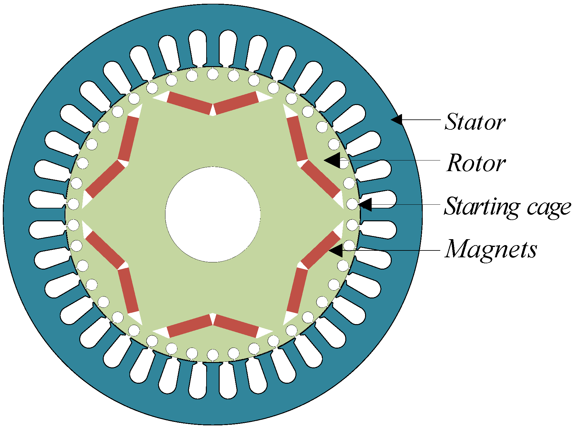
2. Motor Topology and Equivalent Process

In order to increase the generality and versatility of this study, the LSPMSM is selected as the object of analysis. The use of a squirrel cage starting device for the LSPMSM will affect the magnetic field distribution. Therefore, the magnetic field distribution of the analyzed LSPMSM considers the rotor structures of the magnet synchronous motor and the induction motor to provide ideas for the magnetic field resolution of the two types of motors.
This paper analyzes a motor with built-in V-shaped magnets and squirrel cage, as shown in Figure 1. The motor uses NdFeB material as magnet and has 36 stator slots and 42 cast aluminum stator slots, and the detailed data of the motor is shown in Table 2.

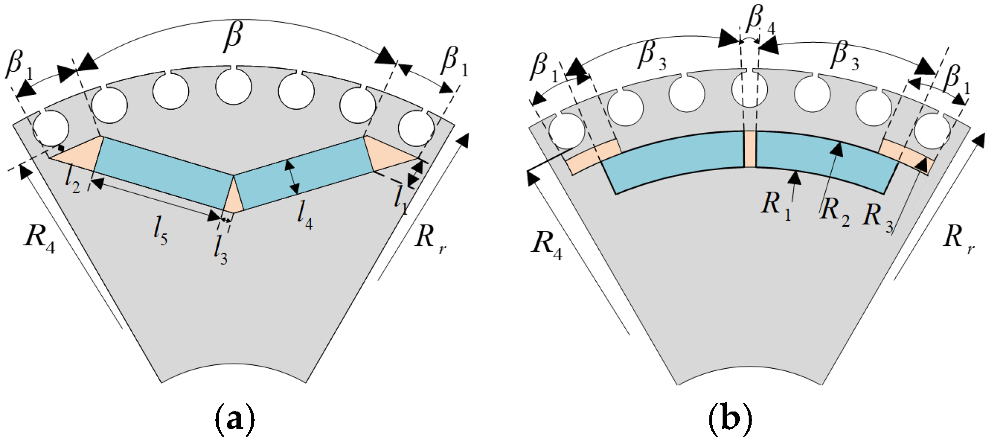
2.1. Simplification of Magnet

To satisfy the boundary conditions of the subdomain solution model and facilitate subsequent analytical modeling, it is necessary to simplify the region of the magnet into a concentric sector. Two key criteria must be met before and after this simplification.
(1)
The air-gap flux generated by the sector-shaped magnet and the rectangular magnet must be equal.
(2)
The pole arc angle, determined by the width angle of the magnet, should be consistent between the sector-shaped magnet and the rectangular magnet.
Following the boundary conditions of the subdomain model solution, the rectangular magnet region of the V-word is considered equivalent to the radially magnetized sector magnet region. A two-dimensional model is established before and after equivalence under the polar coordinate system, as illustrated in Figure 2, where β 3 is the span angle of the equivalent model magnet, β 4 the span angle of the air gap between the magnets, R 1 / R 2 is the radius of the inside/outside of the magnet, R 3 is the outer diameter of the air gap on both sides, and R 4 is the inner diameter of the original model squirrel cage slot.
In order to accurately solve the parameters of the equivalent model, the above equivalence principles are considered as constraints. First, according to the first principle, the thickness of the magnet remains constant before and after the equivalence. Second, according to the principle of flux continuity, the permeance and remanent of the magnet can be deduced under the condition that the equivalent air-gap flux remains unchanged. In addition, combining with the second principle, the magnet spanning angle can be obtained to be unchanged. Finally, considering these conditions, the dimensional parameters of the equivalent magnet can be determined.
The rectangular permeance can be expressed as
G 1 = μ 0 μ 1 l 5 L l 4
where μ 1 is the relative permeance of the magnet; μ 0 is the permeance of the vacuum; L is the length of the motor stator and rotor.
The permeance of the air gap can be expressed as
G g = μ 0 ( R s + R r ) 2 π 2 p L R s R r
where p is the number of pole pairs, R s stator inner diameter.
The remanent of a rectangular magnet can be expressed as
Φ 1 = l 5 L B r
where B r is the remanent magnetization of the magnet.
The original model air-gap flux can be expressed as
Φ g 1 = Φ 1 1 + G 1 / G g
Due to the identical span angles of the inner and outer edges of the fan-shaped magnet and its relatively large radius, when the difference between the inner and outer diameters is small, the arc lengths of the inner and outer edges can be approximated as equal. Therefore, the magnetic circuit of the fan-shaped magnet can be expressed as
G 2 = 0.5 μ 0 μ 1 β 3 ( R 1 + R 2 ) L l 4
The remanent flux of the sector magnet can be expressed as
Φ 2 = 0.5 β 3 ( R 1 + R 2 ) L B r
According to the continuity of the flux, the flux of the air gap after equivalence can be expressed as
Φ g 2 = Φ 2 1 + R g G 2
By the first criterion, the air-gap flux before and after the equivalence is the same, i.e., Φ g 1 is equal to Φ g 2 , which leads to the following equation.
l 5 = 0.5 β 3 ( R 1 + R 2 )
To ensure that the magnet has the same permeance and the same span angle before and after the equivalence, the following equation can be obtained.
l 4 = R 2 R 1
β = 2 β 3 + β 4
In order to minimize the error caused by the equivalence, the air region between the magnets before and after the equivalence can be regarded as the same, and the value of β 4 can be obtained by the following equation.
β 4 = 2 l 3 R 1 + R 2
In addition, the air gap on both sides of the magnet not only generates leakage magnetism, but also determines the path of the magnetic flux, which will cause the air-gap magnetic field to change. In order to ensure the accuracy and avoid the potential unreliability brought by the equivalence, the key features of the initial model should be left unchanged as much as possible during the simplification process: one, the air-gap domain spanning angle does not change before and after the equivalence; and two, the magnetic flux paths and flux densities are unchanged between the air-gap domains and the bottom of the cage slot. Considering the above influencing factors and the need to satisfy the boundary conditions of Poisson’s and Laplace’s equations, the air-gap region on both sides of the magnet is equivalent to a sector-shaped region, as shown in Figure 3. The equivalent air-gap region has an inner diameter of R 2 , an outer diameter that remains unchanged, and a span angle of β 1 ( β 1 is the width of the original model air gap).
The above derivation process, under the guarantee of the magnetic field distribution before and after the equivalence is basically unchanged, simplifies the rectangular magnet, the two sides of the air gap and the magnetic bridge into a sector-shaped region, which satisfies the standard boundary conditions of Poisson’s and Laplace’s equations, so as to facilitate the solving of the sub-domain equations of the region of the magnet.

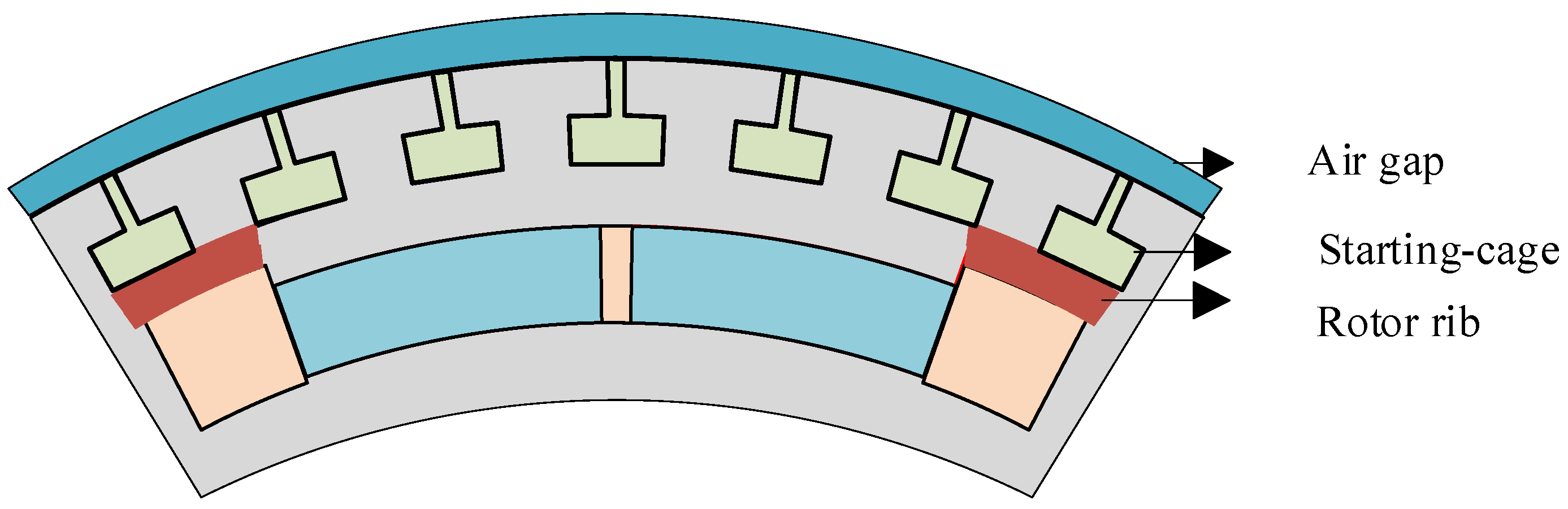
2.2. Simplification of Squirrel Cage Slots

The simplification of the connecting region of the rotor squirrel cage needs to satisfy the condition of the subdomain solution that the simplified shape is a sector-shaped region, and it also needs to ensure that the permeance of this part is the same before and after the equivalence.
The rotor cage slot connection area of the original model is irregularly shaped and the magnetic permeance calculation is complicated. In the equivalence process, the influence of the slots and slots’ mouths on the magnetic field of the air gap needs to be considered to minimize the error caused by the equivalence. Therefore, the squirrel cage slot connection area is divided into two sectors, inner and outer, with the outer sector considering the influence of the slot opening area on the motor and the inner sector ensuring the role of the cage slot area on the magnetic field distribution.
In the calculation of the magnetic permeance, due to the equivalence of the two sectors after the small difference between the inner diameter and outer diameter of the region, the two arc lengths are approximately equal, the sector permeance of the solution is equivalent to the solution of the rectangular magnetic permeance. The magnetic circuit of the two rectangular regions belongs to the series relationship, and the reluctance of the equivalent model is the sum of the two rectangular reluctances. The cross-sectional area of the magnetic circuit of the original model will be changed under the same path, and the reluctance of the connection area of the squirrel cage slot can be obtained by replacing the cross-sectional area of the magnetic circuit of the sector area with the average cross-sectional area of the magnetic circuit of the original model.
The reluctance in the connecting region of the squirrel cage slots of the original and equivalent models can be expressed as
R z = 4 r μ 0 μ z ( m 2 + m 1 ) L
R z 1 = n 2 μ 0 μ z m 1 L + n 1 μ 0 μ z m 2 L
where μ z is the relative permeance of the rotor core; m 1 is the maximum width of the cage slot connection area; m 2 is the minimum width of the cage slot connection area; r is the radius of the cage slot; n 1 is the length of the magnetic circuit in the outer sector; n 2 is the length of the magnetic circuit in the inner sector.
The equivalence of the cage slot connection region is illustrated in Figure 4, and the dimensions of the two sectors after the equivalence, i.e., the values of n 1 and n 2 = 2 r n 1 , are derived from the fact that the magnetoresistance is the same before and after the equivalence, i.e., R z = R z 1 .

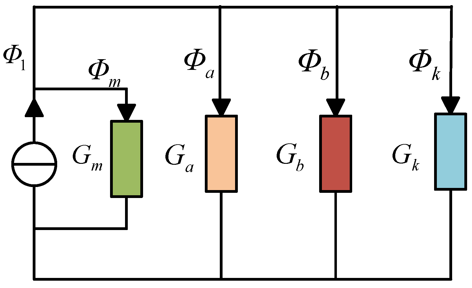
2.3. Magnetic Bridge Saturation

The magnetic bridge serves two principal functions. Firstly, it ensures the strength of the rotor and prevents the magnets from being dislodged from the rotor during high-speed rotation, which could cause structural damage. Secondly, it plays a crucial role in regulating the distribution of the magnetic field, which can effectively control the flow path of the magnetic lines of force. The establishment of a reliable analytical model of the magnetic field and consideration of the saturation effect play a pivotal role in the prediction of the magnetic field distribution of the motor. In general, although the permeance in the saturation region varies with position, the resulting error is relatively minor. Conversely, the leakage flux passes through the magnetic bridge, resulting in a significant difference in the permeance in the bridge region compared to the other regions of the rotor. Consequently, the rotor can be divided into two distinct regions: the unsaturated region and the saturated region with constant permeance. An equivalent model of the rotor at the magnetic bridge is presented in Figure 5. The span angle of the saturated region is related to the width of the bridge in the original model as follows
γ = β 1 + 2 ( R 4 R 3 ) R 4
where β1 is the width of the original model magnetic bridge.
To satisfy the requirements for solving Poisson’s and Laplace’s equations, it is necessary to assume constant permeability in the saturated region of the magnetic bridge in the equivalent model. The nonlinearity of saturated magnetic bridges poses a challenge, which can be effectively addressed using the iterative method to calculate the magnetic permeability of magnetic bridges. Prior to applying the iterative method, the iterative variable must be determined, which in this case is the magnetic permeability of the magnetic bridge. In this paper, a generalized equivalent magnetic circuit model of the motor is established using the equivalent magnetic circuit method, as illustrated in Figure 6. The values of G m ,   G a ,   G b ,   G k and Φ 1 , Φ m , Φ a , Φ b , Φ k represent the permeability of the magnet, the permeability of the air gap, the permeability of the magnetic bridge, the permeability of the inner air gap, and the flux of each branch, respectively.
The iterative method comprises the following steps: firstly, the flux density in the saturation region of the magnetic bridge is set to B b . Secondly, the magnetic field intensity is determined using the B H curve method with known rotor material. Subsequently, the magnetic circuit model is employed to calculate the reluctance and flux, with all the reluctance and flux within the model being calculated. Subsequently, iterative calculations are performed. In each iteration, the discrepancy between the magnetic flux calculated in the previous iteration and the result of the current iteration is evaluated. Should the discrepancy exceed a predefined threshold, the value of B b is then incrementally adjusted. The process is repeated until the iteration results satisfy the predefined error margin requirements. Once the conditions have been satisfied, the permeability of the bridge in the saturated region can be determined. Finally, in order to facilitate a more complete understanding of the entire process of calculating permeability in the saturated region, a flowchart is provided, as shown in Figure 7.

3. Subdomain Model

3.1. Assumptions

In order to facilitate the solution of the model, the following assumptions need to be made:
  • The entire structure stator and rotor (except the bridge) have infinite permeance, and saturation is considered only in the rotor magnetic bridge
  • The effect of the end windings is neglected.
  • Magnets have linear demagnetization properties and are fully magnetized in the direction of magnetization.

3.2. Partial Differential Equations

After equating the regions of the rotor, nine subdomains of the LSPMSM are obtained, as shown in Figure 8, and they are as follows: sector magnet (region I ), air gap on both sides of the magnets (region I I ), magnetic bridge (region I I I ), left slot of the rotor (region I V ), right slot of the rotor (region V ), slot opening of the rotor (region V I ), air gap (region V I I ), slot opening of the stator (region V I I I ), and stator slot (region I X ).
The vector magnetic potential of the subdomain satisfies
2 A r 2 + 1 r A r + 1 r 2 2 A α 2 = μ 0 r ( M α + r M α r M r α )
where A is the vector magnetic potential; M r and M α are the radial and tangential components of the magnetization intensity; and μ 0 is the vacuum permeance.
The region I vector magnetic potential satisfies
2 A r 2 + 1 r A r + 1 r 2 2 A α 2 = μ 0 r M r α
The vector magnetic potentials of the other regions satisfy
2 A r 2 + 1 r A r + 1 r 2 2 A α 2 = 0

3.3. General Solutions

Assuming α = 0 at the centers of the two magnetic poles and resolving the model within α [ 0 , π / p ] , the general solution for the vector magnetic potential A can be found by the method of separated variables due to the symmetry of the model and the combination of the boundary conditions, periodicity, and several assumptions mentioned above. The specific process is described in Appendix A.
A I ( r , α ) = A 1 ln r + B 1 + a C 1 ( r R 2 ) a π β 3 + D 1 ( r R 1 ) a π β 3 + 2 μ 0 r M I r [ cos ( a π ) 1 ] β 3 ( ( a π β 3 ) 2 1 ) cos a π β 3 α α I + β 3 2
where α I / β 3 is the center position angle/span angle of region I , a = 1 , 2 , 3 .
A I I ( r , α ) = A 2 ln r + B 2 + b C 2 ( r R 3 ) b π β 2 + D 2 ( r R 2 ) b π β 2 cos b π β 2 α α I I + β 2 2
where α I I / β 2 is the center position angle/span angle of region I I , b = 1 , 2 , 3 .
A I I I ( r , α ) = A 3 ln r + B 3 + c C 3 ( r R 4 ) c π γ + D 3 ( r R 3 ) c π γ cos c π γ α α I I I + γ 2
where α I I I / γ is the center position angle/span angle of region I I I , c = 1 , 2 , 3 .
A I V ( r , α ) = A 4 ln r + B 4 + d C 4 ( r R 5 ) d π γ 2 + D 4 ( r R 4 ) d π γ 2 cos d π γ 2 α α I V + γ 2 2
where α I V / γ 2 is the center position angle/span angle of region I V , d = 1 , 2 , 3 .
A V ( r , α ) = A 5 ln r + B 5 + e C 5 ( r R 5 ) e π γ 2 + D 5 ( r R 4 ) e π γ 2 cos e π γ 2 α α V + γ 2 2
where α V / γ 2 is the center position angle/span angle of region V , e = 1 , 2 , 3 .
A V I ( r , α ) = A 6 ln r + B 6 + f C 6 ( r R r ) f π γ 1 + D 6 ( r R 5 ) f π γ 1 cos f π γ 1 α α V I + γ 1 2
where α V I / γ 1 is the center position angle/span angle of region V I , f = 1 , 2 , 3 .
A V I I ( r , α ) = g A 7 ( r R s ) g + B 7 ( r R r ) g cos g α + g C 7 ( r R s ) g + D 7 ( r R r ) g sin g α
where α V I I is the center position angle/span angle of region V I I , g = 1 , 2 , 3 .
A V I I I ( r , α ) = A 8 ln r + B 8 + h C 8 ( r R 6 ) h π δ 1 + D 8 ( r R s ) h π δ 1 cos h π δ 1 α α V I I I + δ 1 2
where α V I I I / δ 1 is the center position angle/span angle of region V I I I , h = 1 , 2 , 3 .
A I X ( r , α ) = A 9 ln r + B 9 + i C 9 ( r R 7 ) i π δ 2 + D 9 ( r R 6 ) i π δ 2 cos i π δ 2 α α I X + δ 2 2
where α I X / δ 2 is the center position angle/span angle of region I X , i = 1 , 2 , 3 .
A I A I X represents the region I to region X vector magnetic potential; A 1 A 9 , B 1 B 9 , C 1 C 9 , D 1 D 9 represent the coefficients to be determined for each region; a i represents the number of harmonics in each subdomain.

3.4. Boundary Conditions

The vector magnetic potential A and tangential magnetic field intensity H θ are continuous at the interface between different subdomains. The following boundary conditions are satisfied.
The boundary condition at the interface of region I , I I at R 2 can be expressed as
A I ( R 2 , α ) = A I I ( R 2 , α )           α I I β 2 2 α α I + β 3 2 H I α ( R 2 , α ) = H I I α ( R 2 , α )           α I I β 2 2 α α I + β 3 2
The boundary condition at the interface of region I I , I I I can be expressed as
A I I ( R 3 , α ) = A I I I ( R 3 , α )           α I I β 2 2 α α I I + β 2 2 H I I α ( R 3 , α ) = H I I I α ( R 3 , α )           α I I β 2 2 α α I I + β 2 2
The boundary conditions at the interface of region I V , V and region I I I at R 4 can be expressed as
A I I I ( R 4 , α ) = A I V ( R 4 , α )           α I I I γ 2 α α I V + γ 2 2 H I I I α ( R 4 , α ) = H I V α ( R 4 , α )           α I I I γ 2 α α I V + γ 2 2 A I I I ( R 4 , α ) = A V ( R 4 , α )           α V γ 2 2 α α I I I + γ 2 H I I I α ( R 4 , α ) = H V α ( R 4 , α )           α V γ 2 2 α α I I I + γ 2
The boundary condition at the interface of region I V , V and V I can be expressed as
A I V ( R 5 , α ) = A V I ( R 5 , α )           α V I γ 1 2 α α V I + γ 1 2 A V ( R 5 , α ) = A V I ( R 5 , α )           α V I γ 1 2 α α V I + γ 1 2   H I V α ( R 5 , α ) = H V I α ( R 5 , α )           α V I γ 1 2 α α V I + γ 1 2 H V α ( R 5 , α ) = H V I α ( R 5 , α )           α V I γ 1 2 α α V I + γ 1 2
The boundary condition at the interface of region V I , V I I can be expressed as
A V I α ( R r , α ) = A V I I α ( R r , α )           α V I γ 1 2 α α V I + γ 1 2 H V I α ( R r , α ) = H V I I α ( R r , α )           α V I γ 1 2 α α V I + γ 1 2  
The boundary condition at the interface of region V I I , V I I I can be expressed as
A V I I ( R s , α ) = A V I I I ( R s , α )           α V I I I δ 1 2 α α V I I I + δ 1 2 H V I I α ( R s , α ) = H V I I I α ( R s , α )           α V I I I δ 1 2 α α V I I I + δ 1 2
The boundary condition at the interface of region V I I I , I X can be expressed as
A V I I I ( R 6 , α ) = A I X ( R 6 , α )           α V I I I δ 1 2 α α V I I I + δ 1 2 H V I I I α ( R 6 , α ) = H I X α ( R 6 , α ) α V I I I δ 1 2 α α V I I I + δ 1 2
The specific solution process is shown in Figure 9.

3.5. No-Load Electromagnetic Performance

After determining the vector magnet potential equations for each subdomain, the Fourier series expansion of the equations is combined with the joint system of equations by combining the periodicity and symmetry through the boundary conditions between the subdomains, and the coefficients to be determined for the generalization of each subdomain are solved. Finally, the key electromagnetic performance parameters can be obtained.
The analytical expressions for tangential and radial air-gap flux density are given by
B VII α ( r , α ) = g g ( A 7 r g 1 R s g B 7 r g 1 R r g ) cos ( g α ) g g ( C 7 r g 1 R s g D 7 r g 1 R r g ) sin ( g α )
The no-load EMF expression is given by
E = d ψ d t
where Ψ is the total magnetic flux in each phase of the winding and can be expressed by the following equation
ψ = N B V I I r d S
where N is the number of series turns of each phase winding and S is the area of the winding region each phase.
The cogging torque can be calculated by Maxwell stress tensor, and torque can be expressed as
T = L R g 2 μ o B V I I r ( R g , α ) B V I I α ( R g , α ) d α
where Rg represents the average radius of the air gap.

4. Calculation Results and Analysis

To validate the accuracy of the subdomain model establishment and analytical calculation method, a comparative study is conducted using finite element and analytical methods to solve the electromagnetic performance of the LSPMSM shown in Figure 1. The B-H curve of the iron core is shown in Figure 10. The radial air-gap flux density, tangential air-gap flux density, FFT results, no-load back electromotive force, and magnetic circuit are analyzed and compared between the two methods to verify the correctness of the calculation results.

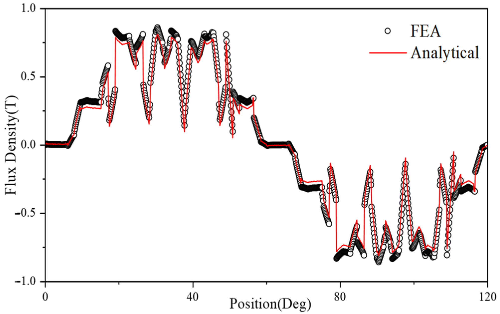
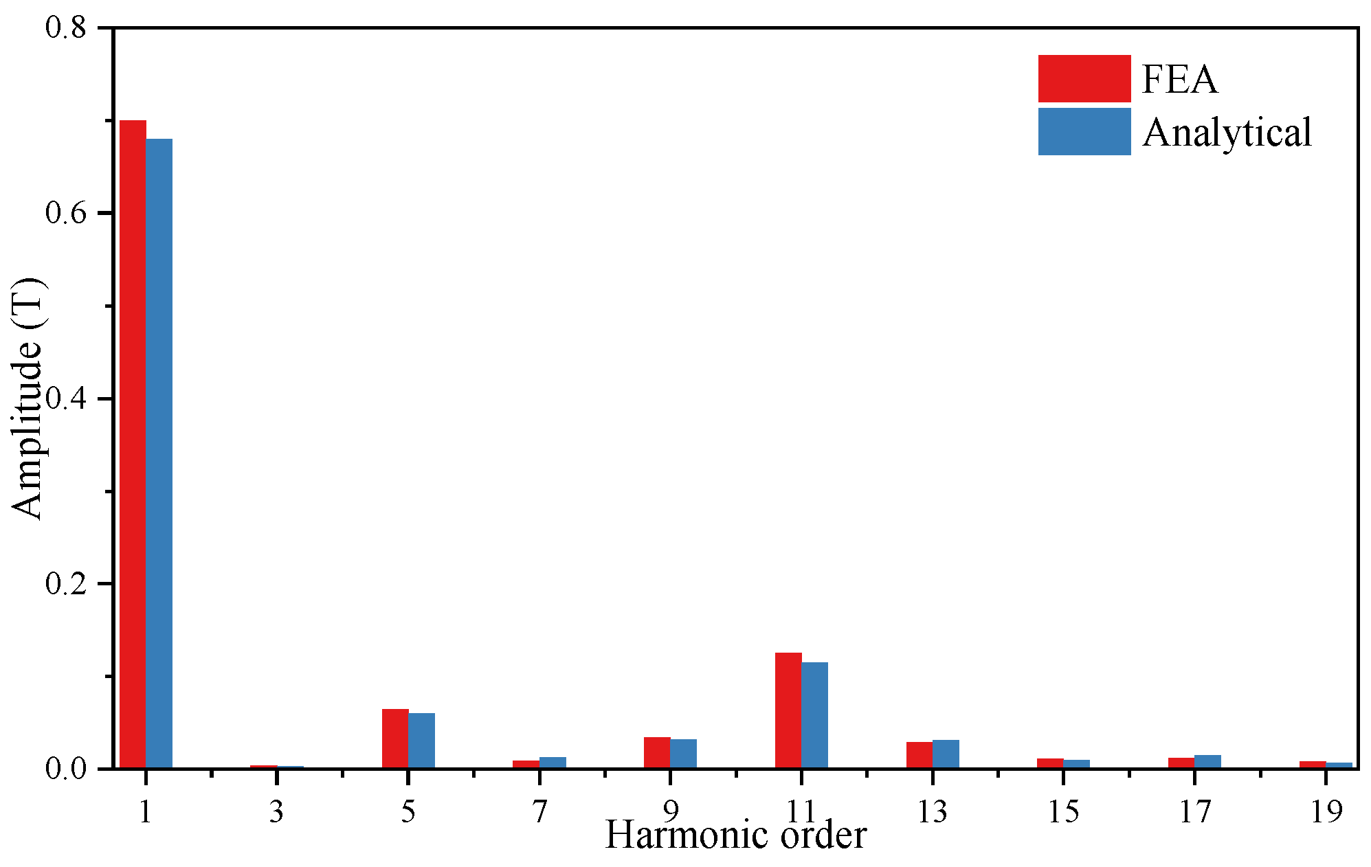
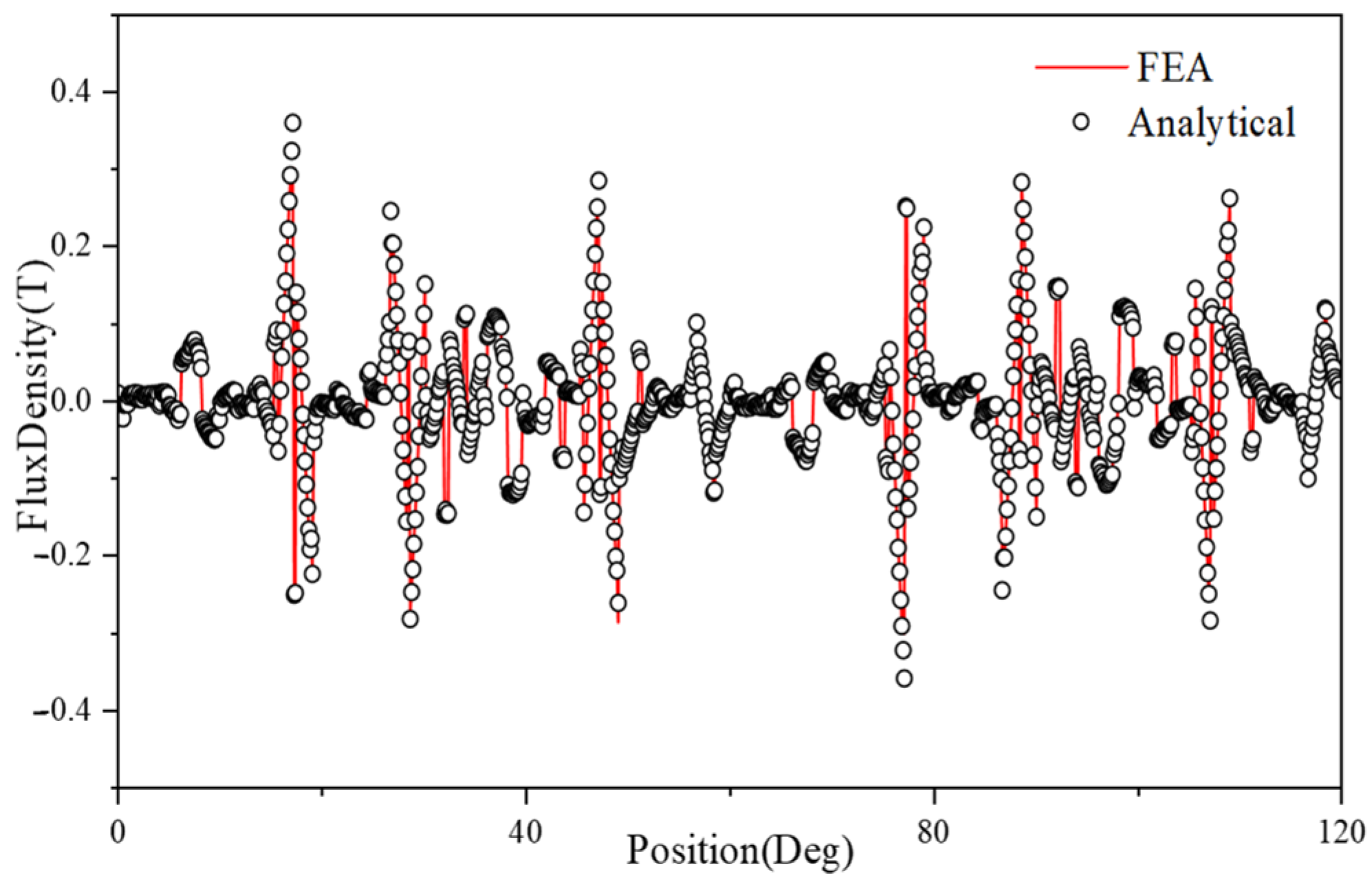
4.1. Air-Gap Flux Density

The comparison of the radial air-gap flux density obtained by finite element and analytical methods is shown in Figure 11. The amplitude of the flux density at the stator tooth and slot positions exhibits a small error, while the results at other positions are basically identical. Furthermore, the radial air-gap flux density obtained by both methods is subjected to Fourier decomposition, and the results are shown in Figure 12. The first harmonic showed a 2.8% error, the ninth had 5.8%, and the thirteenth registered 5.1%. These results indicate that while both methods diverge more at higher harmonics, the 13th harmonic sees a slight decrease in error. Such data guides researchers in choosing the optimal method for specific harmonic analysis. Calculate the root mean square errors of the radial and tangential magnetic flux densities, and the obtained results are 0.0429 and 0.1583, respectively. The analytical and finite element results of the tangential component of the air-gap flux density are also in good agreement, as shown in Figure 13. When considering the influence of magnetic bridge saturation, the analytical calculation assumes a uniform relative permeability of the magnetic bridge, resulting in calculation errors. However, the overall trend of the results is consistent, which verifies the correctness and rationality of the improved analytical method that takes into account the saturation effect.

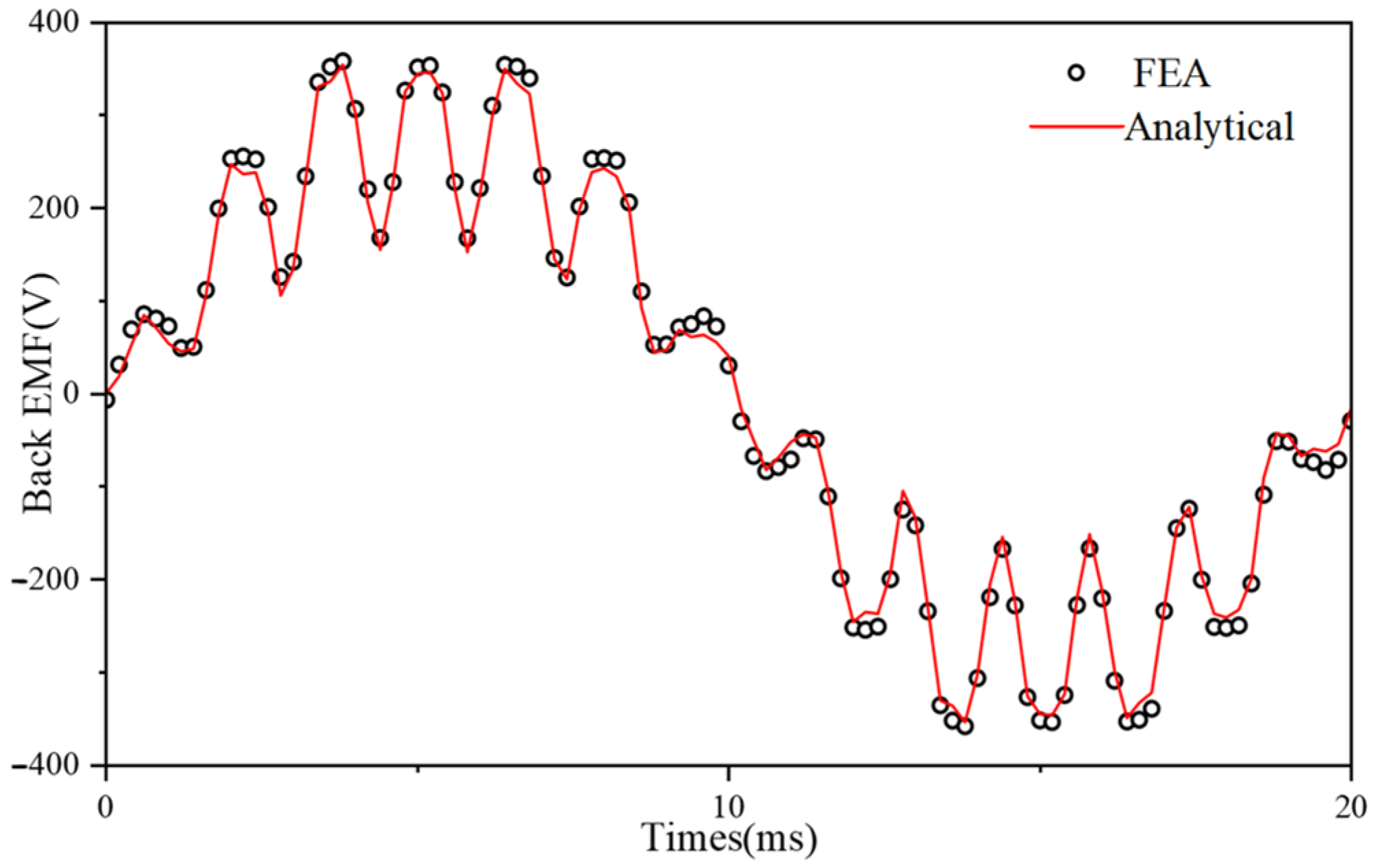
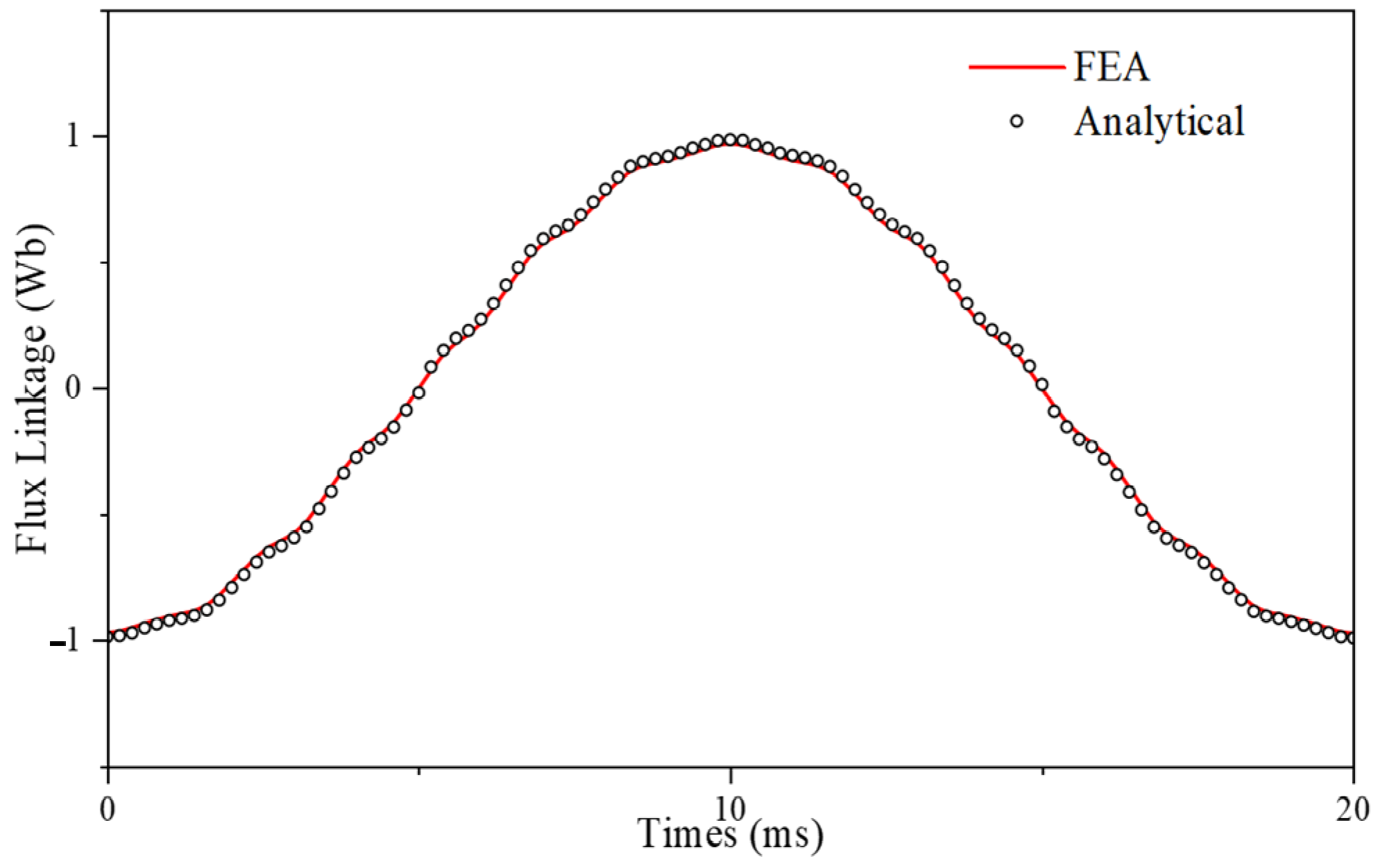
4.2. Flux Linkage and Back EMF

A comparative analysis of the no-load EMF waveforms obtained by the finite element and analytical methods is presented in Figure 14. The results show that the amplitude error of the no-load back EMF calculated by the analytical method is approximately 2% compared to the finite element method. The FFT decomposition of the waveforms obtained by both methods is shown in Figure 15, revealing certain errors at harmonic orders of three, five, nine, and eleven. This discrepancy can be attributed to two factors: (1) the equivalent structure of the motor in the improved analytical model contains errors, and (2) the assumptions made in the analytical solution led to differences with the finite element results. Nevertheless, the error in the analytical no-load back EMF is relatively small. The waveform of the flux linkage is shown in Figure 16. The calculation errors of the two methods are 1%, which is within the acceptable range in engineering practice. This further demonstrates the effectiveness of the analytical method.
The amplitude differences in each electromagnetic parameter between the two methods are taken as the maximum deviations, and the deviation rates are calculated, as shown in Table 3. Through the analysis of the above electromagnetic performance parameters, it is concluded that although there are certain errors between the analytical method and the finite element method, the errors meet the engineering requirements. Furthermore, when solving the electromagnetic parameters of the motor, both methods are within the required error range, and the analytical method not only requires relatively less computation time but also consumes fewer resources. Moreover, a single model can be applied to solve the electromagnetic parameters of motors of the same type.

4.3. Computational Time

The FEA software used in this paper is Ansys EM2021. In order to improve calculation efficiency, 1/6 motor model is calculated, and the number of meshes in the model is 10214. The solution time of FEA is 163 s, and that of the proposed method is 23 s [Intel Core i3-7100F @ 3.90 GHz CPU, 16.0 GB RAM].

5. Conclusions

This paper proposes an improved analytical model for line-starting permanent magnet synchronous motors, addressing the challenges of magnetic field analysis in motors with built-in permanent magnets and line-starting cages. The model is applied to a V-type internal permanent magnet motor with a special rotor structure, featuring a V-shaped embedded permanent magnet, a line-starting cage, and a unique slot shape. By employing the subdomain method and equivalent magnetic circuit method, the no-load electromagnetic performance of the line-starting permanent magnet synchronous motor is calculated. The proposed model not only resolves the issue of satisfying standard boundary conditions for rotor topology but also considers the impact of magnetic bridge saturation.
To validate the accuracy of the proposed improved model, the analytical results of air-gap flux density, back EMF, and magnetic flux are compared with those obtained from finite element analysis. The results show good agreement, with errors within 6% for air-gap flux density, and back EMF amplitude and flux linkage meeting engineering requirements. Furthermore, the proposed improved model exhibits strong engineering practicality and versatility, offering high computational speed and accuracy while being applicable to most internal permanent magnet motors with rotor slots.

Author Contributions

Methodology, J.L.; Formal analysis: J.L. and Y.Z.; Resources: J.L. and Y.S.; software: Y.S.; supervision: Y.S. and M.W.; validation: Y.Z.; writing—original draft: Y.Z.; writing—review and editing: M.W. All authors have read and agreed to the published version of the manuscript.

Funding

This work was supported by the Fundamental Research Foundation for Universities of Heilongjiang Province (2021-KYYWF-0749 and 2021-KYYWF-0746).

Data Availability Statement

Data are contained within the article.

Conflicts of Interest

Author Jinhui Liu was employed by the company Shandong Lijiu Electrical Machinery. Author Yang Zheng was employed by the company Ulanqab Power Supply Branch of Inner Mongolia Electric Power (GROUP). The remaining authors declare that the research was conducted in the absence of any commercial or financial relationships that could be construed as a potential conflict of interest.

Appendix A

According to the method of separation of variables, the vector magnetic potential A a 1 t ( r , α ) can be expressed as
A a 1 t ( r , α ) = R ( r ) δ ( α )
Substituting the above Equation (A1) into the Laplace equation, we can obtain the following:
r 2 R ( r ) + r R ( r ) R ( r ) = δ ( α ) δ ( α ) = λ
Let λ be a constant, and two ordinary differential equations can be obtained:
δ ( α ) + λ δ ( α ) = 0 r 2 R ( r ) + r R ( r ) λ R ( r ) = 0
Equation (A3) satisfies the periodic boundary condition and is a Sturm–Liouville (S–L) problem. Therefore, according to the theory of eigenvalue problems in partial differential equations, the eigenvalues and their corresponding eigenfunctions are
λ 0 = 0 , δ 0 ( α ) = A 0 λ 1 = ( τ m ) 2 = ( m π β ) 2 , δ 1 ( α ) = cos τ m ( α + β 2 α a )
Substituting λ in Equation (A4) into Equation (A3), the general solution can be obtained as
λ 0 = 0 , R 0 ( r ) = A 0 t + B 0 t ln r λ 1 = ( τ m ) 2 = ( m π β ) 2 , R 1 ( r ) = A 1 t r τ m + B 1 t ln r τ m
Linearly superpose Equation (A5) to obtain the general solution of the Laplace equation as
A a 1 t ( r , α ) = R ( r ) δ ( α ) = R 0 ( r ) δ 0 ( α ) + m = 1 R 1 ( r ) δ 1 ( α )
The vector magnetic potential equation can be expressed as
A I I ( r , α ) = A 2 ln r + B 2 + b C 2 ( r R 3 ) b π β 2 + D 2 ( r R 2 ) b π β 2 cos b π β 2 α α I I + β 2 2

References

  1. Palangar, M.F.; Soong, W.L.; Bianchi, N.; Wang, R.-J. Design and Optimization Techniques in Performance Improvement of Line-Start Permanent Magnet Synchronous Motors. IEEE Trans. Magn. 2021, 57, 1–14. [Google Scholar] [CrossRef]
  2. Bu, W.; Fan, Z.; Zhang, J.; Tao, W. Research on the Bearingless Brushless DC Motor Structure with Like-Tangential Parallel-Magnetization Interpolar Magnetic Poles and Its Air-Gap Magnetic Field Analytical Calculation. Actuators 2025, 14, 198. [Google Scholar] [CrossRef]
  3. Yu, Y.; Zhao, P.; Goh, H.; Carbone, G.; Niu, S.; Ding, J.; Shu, S.; Zhao, Z. An Efficient and High-Precision Electromagnetic–Thermal Bidirectional Coupling Reduced-Order Solution Model for Permanent Magnet Synchronous Motors. Actuators 2023, 12, 336. [Google Scholar] [CrossRef]
  4. Meng, B.; Xu, H.; Liu, B.; Dai, M.; Zhu, C.; Li, S. Novel Magnetic Circuit Topology of Linear Force Motor for High Energy Utilization of Permanent Magnet: Analytical Modelling and Experiment. Actuators 2021, 10, 32. [Google Scholar] [CrossRef]
  5. Zhou, K.; Wang, D.; Yu, Z.; Yuan, X.; Zhang, M.; Zheng, Y. Strength Analysis and Design of a Multi-Bridge V-Shaped Rotor for High-Speed Interior Permanent Magnet Synchronous Motors. Actuators 2025, 14, 69. [Google Scholar] [CrossRef]
  6. Jigyasu, R.; Shrivastava, V.; Singh, S. Deep optimal feature extraction and selection-based motor fault diagnosis using vibration. Electr. Eng. 2024, 106, 6339–6358. [Google Scholar] [CrossRef]
  7. Deng, Z.; Ma, T. Analytical Model for Evaluating Unbalanced Electromagnetic Forces in Switched Reluctance Hub Motors Under Air-Gap Eccentricity. In Proceedings of the WCX SAE World Congress Experience, Detroit, MI, USA, 16–18 April 2024. [Google Scholar]
  8. Yu, M.; Zhang, Y.; Lin, J.; Zhang, P. Analysis and Optimization Design of Moving Magnet Linear Oscillating Motors. Actuators 2025, 14, 81. [Google Scholar] [CrossRef]
  9. Wu, S.; Shi, T.; Guo, L.; Wang, H.; Xia, C. Accurate Analytical Method for Magnetic Field Calculation of Interior PM Motors. IEEE Trans. Energy Convers. 2021, 36, 325–337. [Google Scholar] [CrossRef]
  10. Hou, J.; Geng, W.; Li, Q.; Zhang, Z. 3-D Equivalent Magnetic Network Modeling and FEA Verification of a Novel Axial-Flux Hybrid-Excitation In-wheel Motor. IEEE Trans. Magn. 2021, 57, 1–12. [Google Scholar] [CrossRef]
  11. Ghods, M.; Faiz, J.; Gorginpour, H.; Bazrafshan, M.A.; Nøland, J.K. Equivalent Magnetic Network Modeling of Variable-Reluctance Fractional-Slot V-Shaped Vernier Permanent Magnet Machine Based on Numerical Conformal Mapping. IEEE Trans. Transp. Electrif. 2023, 9, 3880–3893. [Google Scholar] [CrossRef]
  12. MGhods, M.; Gorginpour, H.; Faiz, J.; Bazrafshan, M.A.; Toulabi, M.S. Design and Enhanced Equivalent Magnetic Network Modeling of a Fractional-Slot Spoke-Array Vernier PM Machine with Rotor Flux Barriers. IEEE Trans. Energy Convers 2022, 38, 1060–1072. [Google Scholar] [CrossRef]
  13. An, Y.; Ma, C.; Zhang, N.; Guo, Y.; Degano, M.; Gerada, C.; Bu, F.; Yin, X.; Li, Q.; Zhou, S. Calculation Model of Armature Reaction Magnetic Field of Interior Permanent Magnet Synchronous Motor with Segmented Skewed Poles. IEEE Trans. Energy Convers 2022, 37, 1115–1123. [Google Scholar] [CrossRef]
  14. Cai, Y.; Ni, R.; Zhu, W.; Liu, Y. Modified Approach to Inductance Calculation of Variable Reluctance Resolver Based on Segmented Winding Function Method. IEEE Trans. Ind. Appl. 2023, 59, 5900–5907. [Google Scholar] [CrossRef]
  15. Zhu, Z.Q.; Howe, D.; Bolte, E.; Ackermann, B. Instantaneous Magnetic Field Distribution in Brushless Permanent Magnet DC motors. I. Open-circuit Field. IEEE Trans. Magn. 1993, 29, 124–135. [Google Scholar] [CrossRef]
  16. Hajdinjak, M.; Miljavec, D. Analytical Calculation of the Magnetic Field Distribution in Slotless Brushless Machines with U-Shaped Interior Permanent Magnets. IEEE Trans. Magn. 2020, 67, 6721–6731. [Google Scholar] [CrossRef]
  17. Yan, B.; Li, X.; Wang, X.; Yang, Y.; Chen, D. Magnetic Field Prediction for Line-Start Permanent Magnet Synchronous Motor via Incorporating Geometry Approximation and Finite Difference Method into Subdomain Model. IEEE Trans. Ind. Electron. 2023, 70, 2843–2854. [Google Scholar] [CrossRef]
  18. Liu, F.; Wang, X.; Wei, H.; Xiong, L.; Zhang, X. Prediction of Electromagnetic Performance for IPMSM Based on Improved Analytical Model Considering Saturation Effects. IEEE Trans. Transp. Electrif. 2024, 10, 1128–1144. [Google Scholar] [CrossRef]
  19. Ghahfarokhi, M.M.; Faradonbeh, V.Z.; Amiri, E.; Bafrouei, S.M.M.; Aliabad, A.D.; Boroujeni, S.T. Computationally Efficient Analytical Model of Interior Permanent Magnet Machines Considering Stator Slotting Effects. IEEE Trans. Ind. Appl. 2022, 58, 4587–4601. [Google Scholar] [CrossRef]
  20. Liang, P.; Chai, F.; Yu, Y.; Chen, L. Analytical Model of a Spoke-Type Permanent Magnet Synchronous In-Wheel Motor With Trapezoid Magnet Accounting for Tooth Saturation. IEEE Trans. Ind. Electron. 2019, 66, 1162–1171. [Google Scholar] [CrossRef]
  21. Wu, P.; Sun, Y. A Novel Analytical Model for On-Load Performance Prediction of Delta-Type IPM Motors Based on Rotor Simplification. IEEE Trans. Ind. Electron. 2023, 71, 6841–6851. [Google Scholar] [CrossRef]
  22. Li, S.; Tong, W.; Hou, M.; Wu, S.; Tang, R. Analytical Model for No-Load Electromagnetic Performance Prediction of V-Shape IPM Motors considering Nonlinearity of Magnetic Bridges. IEEE Trans. Energy Convers. 2022, 37, 901–911. [Google Scholar] [CrossRef]
Figure 1. Structure of line-start permanent magnet synchronous motor.
Actuators 14 00294 g001
Figure 2. Magnet model: (a) original magnet, (b) equivalent magnet.
Actuators 14 00294 g002
Figure 3. Air−gap region of the magnetic bridge: (a) original model, (b) equivalent model.
Actuators 14 00294 g003
Figure 4. Squirrel cage slot: (a) original model, (b) equivalent model.
Actuators 14 00294 g004
Figure 5. Equivalent magnetic bridge.
Actuators 14 00294 g005
Figure 6. Equivalent magnetic circuit diagram of the motor.
Actuators 14 00294 g006
Figure 7. Iteration process for calculating magnetic permeance of magnetic bridge.
Actuators 14 00294 g007
Figure 8. The subdomain model of the motor: (a) regional division, (b) structural parameters after division.
Actuators 14 00294 g008
Figure 9. Solution process.
Actuators 14 00294 g009
Figure 10. Nonlinear B-H curve of core material.
Actuators 14 00294 g010
Figure 11. Radial air−gap flux density waveforms of rotor magnetic field.
Actuators 14 00294 g011
Figure 12. FFT decomposition of radial air-gap magnetic density.
Actuators 14 00294 g012
Figure 13. Tangential air−gap flux density waveforms of rotor magnetic field.
Actuators 14 00294 g013
Figure 14. Comparison of back EMF.
Actuators 14 00294 g014
Figure 15. FFT decomposition of back EMF.
Actuators 14 00294 g015
Figure 16. Comparison of flux linkage waveform.
Actuators 14 00294 g016
Table 1. Comparison of the advantages and disadvantages of various methods for magnetic field calculation.
AdvantagesShortcomings
FEAHigh calculation accuracyCalculates long-time consumption, not easy to parameterize.
MECCalculates the saturation effects of each part of the iron core accuratelyThe calculation accuracy depends on the number of magnetic resistance divisions, the difficulty of dynamic magnetic field calculation, and the difficulty of dynamic magnetic field calculation.
Sub + MECHigh calculation accuracy, considers the influence of slotting and core saturation simultaneouslyThe applicability of the model is average.
Table 2. Parameters of the studied LSPMSM.
ParameterSymbolValue (Unit)
Number of pole pairsp3 (/)
Number of stator slotsNs36 (/)
Number of rotor slotsNr42 (/)
Inner radius of statorRS147 (mm)
Outer radius of rotorRr148 (mm)
Outer diameter of stator slotR7149 (mm)
Inner diameter of stator slotR6184 (mm)
Inner diameter of cage slotR4134 (mm)
Width of magnetl522.5 (mm)
Thickness of the magnetl46 (mm)
permeance of air μ 0 4π × 10−7 (H/m)
Axial lengthL110 (mm)
Span angle of the magnet β 0.73 (rad)
Length of the air gap at the outer edge of the magnetl14 (mm)
Length of the air gap at the inner edge of the magnetl31.5 (mm)
Table 3. Comparison of electromagnetic performance.
ItemFEAAnalyticalErrors
Flux Linkage (Wb)0.970.981%
Back EMF (V)3533571.1%
Disclaimer/Publisher’s Note: The statements, opinions and data contained in all publications are solely those of the individual author(s) and contributor(s) and not of MDPI and/or the editor(s). MDPI and/or the editor(s) disclaim responsibility for any injury to people or property resulting from any ideas, methods, instructions or products referred to in the content.

