Article

Optimal Realtime Toolpath Planning for Industrial Robots with Sparse Sensing

by
Enkhsaikhan Boldsaikhan
* and
Cole Birney
Industrial Systems and Manufacturing Engineering Department, Wichita State University, Wichita, KS 67260, USA
*
Author to whom correspondence should be addressed.
Actuators 2025, 14(6), 279; https://doi.org/10.3390/act14060279
Submission received: 22 April 2025 / Revised: 25 May 2025 / Accepted: 5 June 2025 / Published: 7 June 2025

Abstract

Non-contact surface processing does not involve direct contact between the tool and a worksurface. An industrial robot mostly uses preplanned toolpaths to perform non-contact surface processing. A preplanned toolpath may work well in repetitive conditions but may easily become inaccurate and unsafe if the tool needs to follow unknown worksurface variations. Many industrial processes, e.g., painting, coating, and sandblasting, typically involve worksurfaces with unknown variations. This study proposes an optimal toolpath planning method for an industrial robot equipped with end-of-arm distance sensors to automatically guide its tool motion along unknown worksurface variations. The distance sensors facilitate sparse sensing to acquire sparse data that is just enough for the quick and adequate perception of unknown worksurfaces by requiring fewer measurements and less computing. Optimization facilitates the optimality of multi-objective toolpath planning with a customizable value function, where the multiple objectives comprise adapting to unknown worksurface variations and traveling between known tool targets. To validate the proposed toolpath planning method, this study conducts a simulation experiment on a virtual robot with four end-of-arm distance sensors and a workpiece with unknown surface variations. The experimental results indicate that the proposed method is accurate and near-optimal even in the presence of sensor noises.

1. Introduction

Industrial robots are emerging as major autonomous systems for handling various manufacturing tasks that are highly repetitive, difficult, and unsafe to humans [1,2,3]. The International Organization for Standardization (ISO) [4,5] identifies an industrial robot as an automatically controlled, reprogrammable, multipurpose, manipulative system with several reprogrammable axes, which may be either fixed in place or mobile for use in industrial automation applications. An industrial robot mostly uses preplanned toolpaths to perform non-contact surface processing. A preplanned toolpath may work well in repetitive conditions but may easily become inaccurate and unsafe if the tool needs to follow unknown worksurface variations. Many industrial processes, e.g., painting, coating, and sandblasting, typically involve worksurfaces with unknown variations.
Researchers have proposed theoretical methods for robotic toolpath planning [6,7,8,9,10,11,12,13,14,15,16,17,18,19,20,21,22] as well as their practical applications [6,7,8,9,13,14,16,18,23]. Navigation and the precision of toolpaths are practically important as an industrial robot may exhibit positioning errors [24,25] due to uncertain variations involved in the environment. Non-rigid robots with hyper-elastic, soft bodies experience even bigger challenges in terms of navigation, motion precision, stiffness, and compliance [26,27,28,29]. All these challenges in robotics indicate the importance of sensing, which can provide the needed perception of priorly unknown variations in environments, for better navigation and control of robots and autonomous systems.
For robotic non-contact surface processing, contactless sensing is always preferred as it allows a robot to sense surfaces from a distance. There are various contactless sensors (or non-contact sensors), such as vision cameras [30,31,32,33,34,35,36,37,38,39], laser trackers [24,40], Light Detection and Ranging (LiDAR) scanners [41,42], and so on, used in industrial applications. Vision cameras provide ample perception but require fast communication interfaces and extensive data processing. Laser sensors like range sensors, laser trackers, and LiDAR scanners can provide accurate spatial sensing but produce harmful laser beams. Ultrasonic distance sensors are simpler than machine vision cameras and safer than laser beams. They are not affected by the color or transparency of objects but have limitations in terms of acoustic disturbances and short detection ranges.
Researchers have documented various methods for the sensor-based routing and control of industrial robots [9,13,38,39,43,44], mobile robots [30,42,45,46], and aerial robots or drones [34,47,48]. However, these research outcomes mostly focus on solutions with resource-intensive sensing rather than generic solutions with less resource-intensive sensing for baseline perception. An example of resource-intensive sensing is machine vision, which can easily produce abundant data that is costly to compute in real time. In contrast, sparse sensing with simple distance sensors produces sparse data that is just enough for the quick, adequate perception of environments with less computing. In general, sparse sensing [49] is a sensing technique that leverages fewer measurements that are just enough to reconstruct full-field perception. It requires fewer hardware and software resources to provide quick, baseline perception.
There is a noticeable research gap in realtime toolpath planning with sparse sensing in industrial robotics. To bridge this gap, this study proposes an optimal path planning method with sparse sensing for an industrial robot equipped with end-of-arm distance sensors to automatically guide its tool motion along unknown worksurface variations. The end-of-arm distance sensors facilitate sparse sensing for quick, baseline perception. Optimization facilitates the optimality of multi-objective path planning with a customizable value function, where the multiple objectives of path planning comprise adapting to unknown worksurface variations and traveling between known toolpath targets.
To validate the proposed toolpath planning method with sparse sensing, this study conducted a simulation experiment on a virtual robot equipped with end-of-arm distance sensors and a workpiece with unknown surface variations. The simulation experiment systematically demonstrated the proposed method with and without sensor noises.

2. Materials and Methods

2.1. Problem Formulation

An end-effector is a tool that goes on the end of a robot arm. A tool pose defines the tool position and orientation in the reference frame. A robot manipulates its tool pose within the operational or task space of the robot. A robot tool must have a tool reference frame or simply a tool frame, and the tool frame origin is the tool center point or tool control point (TCP), which is the location where the robotic process takes place. A target is a tool pose, and a toolpath or path is a continuous stream of tool poses.
This problem formulation involves an industrial robot with an end-of-arm tool that has four distance sensors and a tool reference frame for non-contact surface processing as illustrated in Figure 1. Adaptive toolpath planning needs to guide the robot TCP along unknown worksurface variations by maintaining relative tool orientation and alignment, while the tool travels between known start and end tool poses. The end tool pose or target also serves as the frame of reference. A toolpath must adapt to unknown worksurface variations along the XZ plane of reference frame, which means an adapted toolpath must be constrained to the XZ plane of reference frame. The relative tool orientation depends on a manufacturing process, i.e., a welding process requires a certain attack angle between the welding tool and the toolpath. In this problem formulation, the robot tool axis, which is the z T axis, needs to be orthogonal to the sensed worksurface for clarity and simplicity.
The four end-of-arm distance sensors have a square arrangement with a diagonal length of l on the sensor plane as shown in Figure 1. This square arrangement is centered at the tool axis, which is the z T axis of the tool frame, and the tool axis is orthogonal to the sensor plane. Moreover, the two diagonals of the square arrangement are parallel to the tool x T axis and the tool y T axis, respectively. All the sensors have the same concentric inclination angle φ , which is assigned to 90 degrees to make each sensor axis orthogonal to the sensor plane for simplicity. Four distance sensors sense the distances— a n , b n , c n , and d n —between the sensor plane points and the sensed worksurface points, respectively, in each timestep n N . The sensor plane is the interface plane between the robot end and the robot tool in Figure 1. The four distance sensors are associated with four customizable reference distances— a r e f , b r e f , c r e f , and d r e f —that signify a desired tool pose relative to a sensed worksurface. These four reference distances define a tool reference plane. In this formulation, let the XY plane of the robot tool frame be the tool reference plane for clarity and simplicity, which implies that all the reference distances are equal to the distance between the sensor plane and the XY plane of the robot tool frame. Note that the sensor plane is parallel to the XY plane of the robot tool frame.
The origin of the robot tool frame is tool center point (TCP), where a non-contact process takes place. The robot tool needs to follow sensed worksurface variations along the XZ plane of the reference frame ( p B ) by maintaining alignment between the tool reference plane (the XY plane of the robot tool frame) and the sensed worksurface, while traveling between known start and end tool poses.
Toolpath P p A ,   p B in (1) is a series of adapted toolpath poses in between given or known start and end tool poses, p A R 6 and p B R 6 , respectively.
P p A ,   p B = p n R 6     p 0 = p A ;   p N = p B ;   N N ; n = 0 ,   1 , ,   N
In (1), n and N are a timestep index and the finite number of timesteps, respectively. In each timestep n, realtime toolpath planning produces an adapted tool pose p n R 6 . Each tool pose or target p n consists of the x, y, z coordinates of the TCP and the θ x , θ y , θ z Euler angles with respect to the reference frame in Figure 1. In every timestep, the adaptive toolpath planner must estimate the next pose p ^ n + 1 using the current tool pose p n and a tool pose correction p n as formulated in (2). The tool pose correction p n in (2) consists of a correction p n | s relative to the sensed worksurface and a correction p n | B n relative to an incremental tool target p ^ B n . Let p n | B n = p be a known constant as a uniform increment in the direction of the final tool target p B . Figure 2 shows the geometry of an incremental tool target p ^ B n = p n + p n | B n . Moreover, Figure 2 illustrates the vector operations in (2) for estimating the next pose p ^ n + 1 .
p ^ n + 1 = p n + p n = p n + p n | s + p n | B n
Finally, the problem formulation boils down to finding the tool pose correction p n and its components, p n | s and p n | B n , to estimate the next tool pose p ^ n + 1 based on the current tool pose p n in every timestep. This study proposes a numerical solution to this problem by using realtime error tracking with linear quadratic regulation as outlined in Section 2.2.

2.2. Realtime Error Tracking with Linear Quadratic Regulation

The end-of-arm distance sensors in Figure 1 provide four distance sensor readings— a n , b n , c n , and d n —in every timestep n. The four distance sensors are associated with four customizable reference distances— a r e f , b r e f , c r e f , and d r e f —that signify a desired tool pose relative to a sensed worksurface. These four reference distances define a tool reference plane. In this study, the XY plane of the robot tool frame is the tool reference plane for clarity and simplicity, which implies that all the four reference distances are equal to the distance between the sensor plane and the XY plane of the robot tool frame. The deviations of four distance readings from their respective reference distances are a n | r e f , b n | r e f , c n | r e f , and d n | r e f as derived in (3).
a n | r e f b n | r e f c n | r e f d n | r e f T = a n b n c n d n T a r e f b r e f c r e f d r e f T
Besides tracking worksurface variations, the robot tool must reach the known final tool target p B in Figure 1. The final tool target p B also serves as the frame of reference or reference frame for convenience. The TCP coordinates of the current tool pose p n are x n , y n , and z n . Since the final tool target p B is located at a remote distance, an incremental tool target p ^ B n is used at a uniform incremental distance from the current pose p n in the direction of the final tool target p n in each timestep as shown in Figure 2. The TCP coordinates of the current tool pose p n that is relative to an incremental tool target p ^ B n are x n | B n , y n | B n , and z n | B n , which are incremental tool target errors, according to (4).
x n | B n y n | B n z n | B n T = x n y n z n T x B n y B n z B n T
The sensed deviations a n | r e f , b n | r e f , c n | r e f , and d n | r e f as well as the incremental tool target errors x n | B n , y n | B n , and z n | B n constitute an error vector e n R 7 in (5).
e n = e n 1 e n 2 e n 3 e n 4 e n 5 e n 6 e n 7 T = = a n | r e f b n | r e f c n | r e f d n | r e f x n | B n y n | B n z n | B n T
Figure 3 demonstrates a tool θ y angle as a pitch angle between the tool XY plane and a worksurface using the sensed deviations, a n | r e f and c n | r e f . Likewise, a tool θ x angle can also be identified as a roll angle between the tool XY plane and a worksurface using the sensed deviations, b n | r e f and d n | r e f . Adaptive toolpath planning aims to maintain orientation alignment between the tool XY plane and a sensed worksurface using these two tool angles for tool pose corrections. The sensor inclination angle φ in Figure 1 is 90 ° . The sensitivity factor η is a heuristic scalar between 0 and 1, where 0 means no sensitivity, and 1 means full sensitivity. It can be used to lessen the amplifying effects of the two sensed deviations on the pivot point, which is the TCP. It can also be used to lessen the effects of sensor noises. The η sensitivity factor is 0.5 in this study.
The goal of adaptive toolpath planning is to minimize the error vector e n with less effort. Therefore, the proposed approach involves a first-order error tracking model presented in (6).
e n + 1 = e n + u n
In (6), a control input vector u n R 7 aims to minimize the error vector e n in each timestep n. It is derived from the error vector e n according to (7), (8), and (9) using a control gain matrix K R 7 × 7 that is a predefined diagonal matrix of the scalar gains K s and K B in (8) and (9). The gain K s is used to regulate the deviations of the four sensor readings from their respective reference distances, and the gain K B is used to guide the TCP motion in the direction of the known final tool target p B .
u n = K e n
K = d i a g ( K s , K s , K s , K s , K B , K B , K B ) R 7 × 7
u n = u n 1 u n 2 u n 3 u n 4 u n 5 u n 6 u n 7 T =                             = K s a n | r e f K s b n | r e f K s c n | r e f K s d n | r e f K B x n | B n K B y n | B n K B z n | B n T
The tool pose correction p n in (2) consists of a correction p n | s relative to the sensed surface and a correction p n | B n relative to an incremental tool target p ^ B n . Hence, the formulas in (10) and (11), respectively, derive p n | s and p n | B n from u n in every timestep n. In (10), p n | s z is the average of the tool–worksurface distance corrections, u n 1 , u n 2 , u n 3 , and u n 4 to align the toolpath TCP with a sensed worksurface. The tool orientation corrections, p n | s θ y and p n | s θ x , are derived from u n by using the approach demonstrated in Figure 3, where the sensed deviations, a n | r e f , b n | r e f , c n | r e f , and d n | r e f , are replaced by the tool–worksurface distance corrections, u n 1 , u n 2 , u n 3 , and u n 4 , respectively, in (10) to align the tool reference plane with a sensed worksurface. The η sensitivity factor in (10) is 0.5 in this study. In (11), the TCP corrections, u n 5 , u n 6 , and u n 7 , are applied to the tool pose correction p n | B n to reach the incremental tool target p ^ B n . Figure 4 provides an overall schematic of realtime error tracking with linear quadratic regulation for adaptive toolpath planning with sparse sensing, where p ˙ r e f is a reference tool speed that encompasses a predefined TCP speed and a predefined tool angular speed.
p n | s = p n | s x p n | s y p n | s z p n | s θ x p n | s θ y p n | s θ z = 0 0 u n 1 + u n 2 + u n 3 + u n 4 4 tan 1 η * u n 1 u n 3 l tan 1 η * u n 2 u n 4 l 0
p n | B n = p n | B n x p n | B n y p n | B n z p n | B n θ x p n | B n θ y p n | B n θ z T   = u n 5 u n 6 u n 7 0 0 0 T
The proposed realtime toolpath planning then employs linear quadratic regulation (LQR) to compute the gain matrix K in (8) using a customizable value function ϕ e n ,   π in (12), where π is a control sequence in (13) that steers the error tracking model in (6) from its current state e 0 | n (or e n ) to a final state e | n on an infinite time horizon.
ϕ e n ,   π = t = 0 e t | n T   Q e t | n + u t | n T   R u t | n ;     e 0 | n = e n , Q = Q T 0 ,     R = R T 0
π = u t | n   R 6   |     t = 0 , 1 ,   ,  
In (12) and (13), t N is a timestep index on an infinite time horizon. Q R 7 × 7 and R R 7 × 7 are customizable state and control weight matrices, respectively. The goal of the optimization problem in (14), which is subject to (6) and (7), is to find an optimal control sequence π * to steer the error tracking model in (6) from its current state e 0 | n (or e n ) to an optimal state e | n * that converges to zero on an infinite time horizon.
ϕ e n = min π ϕ e n ,   π π * = argmin π ϕ e n ,   π
To solve the optimization problem in (14) that is subject to (6) and (7), a cost-to-go matrix P R 7 × 7 can be identified using the discrete algebraic Riccati equation (DARE) in (15) on an infinite time horizon.
P = Q + P P R + P 1 P ; P = P T 0
After solving (15) for P , a time-invariant gain matrix of K can be found according to formula in (16) for the realtime error tracking model in (6) and its control input in (7).
K = R + P 1 P
Many researchers including Al Tamimi et al. [50], Rawlings et al. [51], and Scokaert et al. [52] documented distinct variants of optimal control and linear quadratic regulation with in-depth mathematical derivations and proofs on stability and controllability. Their research papers can provide more theoretical details for further reading.

2.3. Experimental Settings

This study involves a simulation experiment on an industrial robot with end-of-arm distance sensors and a workpiece with unknown surface variations to demonstrate the proposed toolpath planning with sparse sensing using RobotStudio® 2024, which is an industrial robot programming and simulation program [53]. RobotStudio® 2024 has digital engineering capabilities of robot modeling, programming, and simulation with virtual sensors and devices. The simulation experiment employed a virtual ABB IRB-1200 robot with end-of-arm distance sensors and a workpiece with unknown surface variations as modeled in RobotStudio® 2024. Figure 1b portrays the setup of the simulation experiment. The robot tool frame with the tool center point (TCP) was arranged at 200 mm from the sensor plane along the tool z T axis. The diagonal length l of the sensor square arrangement was 40 mm. The sensor inclination angle φ was 90 degrees for all four sensors. The robot was tasked to start from a known start pose and then reach a known final tool target by aligning the TCP with unknown worksurface variations and maintaining tool orthogonality relative to the sensed surface. It is assumed that the TCPs of both the start and the end poses are predefined worksurface points. The end pose served as the frame of reference. The p ˙ r e f reference tool speed of simulation comprised 100 mm/s as a TCP speed and 1000 deg./s as a tool angular speed. The p uniform increment of TCP was 10 mm. The timestep of the simulation was 0.5 s. The data sampling rate was 125 Hz.
This study used sensor noises to test the robustness of the proposed approach. Sensor noises can have various sources, such as vibrations, environmental disturbances, sensor calibration errors, etc. To apply noise to the sensor perception, each sensor reading was subjected to a random scalar from a 4 mm range between −2 mm and +2 mm.
To demonstrate customizable optimal toolpath planning, three optimal regulation cases were considered via customized weight matrices in Table 1, where Q   R 7 × 7 and R   R 7 × 7 are error state and control weight matrices, respectively. These weight matrices are used for solving the optimization problem in (14), which is subject to the error tracking model in (6) with the control input in (7). The customizable weights are based on a simple scoring range between 1 and 10, which serves as a handle on intuitively praising or penalizing certain error states and control actions for optimal toolpath planning.
In Case 1, the weights for sensed deviations, which are the first four entries in the diagonal of the error state weight matrix Q , are 1s, while the remaining weights for toolpath target errors are 10s. This means toolpath target errors are more costly to endure than sensed deviations. Also, the weights for sensed deviation control, which are the first four entries in the diagonal of the control weight matrix R , are 10s, while the remaining weights for toolpath target control are 1s. It means sensed deviation control is more costly to execute than toolpath target control. Overall, the Case 1 weights imply that reaching the known toolpath target is the top priority.
In Case 2, the customized weights are all equal to 10s, which means reaching the known toolpath target and following sensed surface variations are equally important.
In Case 3, the weights for sensed deviations, which are the first four entries in the diagonal of the error state weight matrix Q , are 10s, while the remaining weights for toolpath target errors are 1s. It means sensed deviations are more costly to endure than toolpath target errors. Also, the weights for sensed deviation control, which are the first four entries in the diagonal of the control weight matrix R , are 1s, while the remaining weights for toolpath target control are 10s. It means toolpath target control is more costly to execute than sensed deviation control. Overall, the Case 3 weights imply that surface tracking is the top priority.
A time-invariant gain matrix of K was computed according to (16) for each case using the weights in Table 1 and the linear quadratic optimization in (14) that is subject to (6) and (7). Table 2 presents the computed LQR gains. These LQR gains were used to systematically demonstrate optimal toolpath planning with and without sensor noises.

3. Results and Discussion

The simulation experiment involved three optimal realtime toolpath planning cases as specified in Table 1 and Table 2 with and without sensor noises. To apply artificial noise to sensor perception, each sensor reading was subjected to a random number from a 4 mm range between −2 mm and +2 mm. In each case, an industrial robot with end-of-arm distance sensors was tasked to travel between known start and end tool poses by maintaining the tool orthogonality and the TCP alignment with the sensed worksurface as well as the ZX plane of the reference frame. The TCPs of both the start and the end tool poses were worksurface points. The end pose (the final tool target) also served as the reference frame. The p ˙ r e f reference tool speed of simulation comprised 100 mm/s as the TCP speed and 1000 deg./s as the tool angular speed. The p uniform increment of TCP was 10 mm, and the timestep of simulation was 0.5 s. The data sampling rate was 125 Hz.
Reaching the known toolpath target is the top priority in Case 1. Worksurface tracking is the top priority in Case 3. Balancing the Case 1 and Case 3 goals is the priority in Case 2. Figure 5 presents an image sequence of the Case 3 simulation.
The cycle times of Case 1, Case 2, and Case 3 without sensor noises were about 16 s, 18 s, and 23 s, respectively. The total lengths of the Case 1, Case 2, and Case 3 toolpaths without sensor noises were about 848 mm, 852 mm, and 866 mm, respectively. The cycle times of Case 1, Case 2, and Case 3 with sensor noises were about 16 s, 19 s, and 28 s, respectively. The lengths of the Case 1, Case 2, and Case 3 toolpaths with sensor noises were about 848 mm, 855 mm, and 908 mm, respectively. Sensor noises affected Case 3 more than any other cases since sensor-based surface tracking is the top priority in Case 3.
Figure 6, Figure 7 and Figure 8 present comparisons between the toolpath orientation angles of an ideal case and the three cases with and without sensor noises. The ideal case involves ideal tool poses to achieve along an ideal toolpath defined by the intersection between the worksurface and the XZ plane of the reference frame. Figure 9 and Figure 10 present comparisons between the ideal toolpath and the toolpaths of the three cases with and without sensor noises. Figure 11 presents the toolpath TCP errors of the three cases with and without sensor noises. A positive error in Figure 11 means the TCP is above the worksurface, and a negative error means the TCP is below the worksurface.
The results in Figure 6, Figure 7 and Figure 8 indicate that each experimental case was able to accomplish the anticipated optimal path planning goals in accordance with the customized weights specified in Table 1 and the LQR gains in Table 2. The tool θ z angle is nicely maintained at 90 degrees in each of the three cases even in the presence of sensor noises. In comparison with the ideal case and Case 1, both Case 2 and Case 3 produced fairly accurate toolpath orientation angles but longer cycle times since tracking sensed surface variations requires more time to accomplish, especially in Case 3. In contrast, Case 1 produced less-accurate toolpath orientation angles but the shortest cycle time since reaching the known tool target is the top priority of Case 1. This urgency to reach the end target causes insufficient time to accurately track sensed surface variations. Added sensor noises barely affected the performances of Case 1 and Case 2 but noticeably affected the Case 3 performances. Since sensor-based surface tracking is the top priority in Case 3, sensor readings play essential roles in Case 3, which makes it more sensitive to sensor noises. This sensitivity can be reduced by reducing the η sensitivity factor in (10). Note that this study used a sensitivity factor of η = 0.5 . The results in Figure 6, Figure 7 and Figure 8 are summarized in Figure 12, which presents the Root Mean Square (RMS) errors [23] of the tool orientation for the three cases with and without sensor noises. Case 1 produced the largest angular RMS errors in the tool θ x and θ y angles in comparison with the ideal toolpath orientation angles shown in Figure 6 and Figure 7, while Case 3 and Case 2 produced much lower angular RMS errors.
According to Figure 9, Figure 10 and Figure 11, the toolpath TCP coordinates of the three cases eventually converge at zero when the robot tool reaches the final tool target at the end of each process cycle. Note that the final tool target is also the reference frame. Figure 9 shows that the TCP alignment with the XZ plane of the reference frame looks flawless in each of the three cases with and without sensor noises as expected. Figure 10 presents comparisons between the ideal toolpath and the toolpaths of the three cases with and without noises. The results in Figure 9, Figure 10 and Figure 11 are summarized in Figure 13. In terms of tracking unknown surface variations, the toolpaths of Case 3 and Case 2 are the most accurate ones with RMS errors of less than 2.5 mm even in the presence of sensor noises. The Case 3 toolpath has some fluctuations in Figure 10 and Figure 11, especially in the presence of sensor noises. Such unwanted fluctuations can be reduced by reducing the η sensitivity factor in (10). The Case 1 toolpaths with and without sensor noises exhibit noticeable RMS errors of over 7 mm, which is expected since worksurface tracking has a lower priority in Case 1.
Figure 14 presents box-and-whisker plots of the actual toolpath speeds. Each box-and-whisker plot depicts the upper and lower extremes, the upper and lower quartiles, and the median of each dataset. Since the main emphasis of the proposed method is on enhancing the tool pose accuracy of the toolpaths, the proposed method does not regulate tool speeds by letting the robotic system control its tool speeds based on the commanded or reference tool speeds and kinematic constraints. The commanded or reference tool speeds of the simulation experiment were 100 mm/s as a linear speed of the toolpath TCP and 1000 deg/s as an angular speed of toolpath orientation. The actual toolpath speeds of the simulation experiment were lower than the reference tool speeds as the robot tool needed to slow down to apply new sensor-based changes to the tool pose in every timestep of 0.5 s. This limitation can be resolved by tool speed planning with speed interpolation as well as a specific sensor arrangement that allows the robot to sense the worksurface ahead of the tool along the toolpath. Moreover, Model Predictive Control (MPC) can be instrumental in achieving proper tool speed planning. Needless to say, both LQR and MPC are specific variants of optimal control.
The simulation experiment successfully demonstrated the predefined optimal path planning strategies with and without noises. These findings indicate that the proposed toolpath planning method with sparse sensing has the potential to automate non-contact surface processing. In this study, sparse sensing required fewer measurements and less computing than that for standard machine vision. The computational time complexity of sparse sensing was O ( n ) , which was much lower than O ( n × m ) of a standard image convolution algorithm typically used in machine vision, where n and m are the total number of timesteps and the total number of image pixels, respectively. The big O notation is a math notation that describes the limiting behavior of an algorithm or a function when the input argument tends toward infinity.
A limitation of the proposed path planning approach is an inability to deal with worksurface discontinuities, such as edges, holes, pockets, steep protruding surfaces, or sharp ridges. A possible solution to this problem can be smart sensor arrangements along with an intelligent algorithm that can detect surface discontinuities by examining distance sensor readings. Another limitation of the proposed toolpath planning approach is that it regulates the tool pose but not the tool speed. This limitation can be resolved by adding toolpath speed planning with speed interpolation. The future work will focus on resolving these limitations, establishing benchmark datasets for comparisons with other methods, and implementing artificial intelligence for better robot tool motion planning and control.

4. Conclusions

This study proposes an optimal toolpath planning method for an industrial robot equipped with end-of-arm distance sensors to automatically guide its tool motion along unknown worksurface variations. The end-of-arm distance sensors facilitate sparse sensing to acquire sparse data that is just enough for the quick, adequate perception of unknown worksurfaces. Optimization facilitates the optimality of multi-objective toolpath planning with a customizable value function, where the multiple objectives comprise adapting to unknown worksurface variations and traveling between known tool targets. To validate the proposed toolpath planning method with sparse sensing, this study conducted a simulation experiment on a virtual robot equipped with end-of-arm distance sensors and a workpiece with unknown surface variations. Sparse sensing required fewer measurements and less computing than that for conventional machine vision. The simulation experiment successfully demonstrated the predefined optimal strategies with and without sensor noises. These findings indicate that the proposed toolpath planning method with sparse sensing has the potential to automate non-contact surface processing. The future work will focus on adding tool speed planning, establishing benchmark datasets for comparisons with other methods, and implementing artificial intelligence for better robot tool motion planning and control.

Author Contributions

Conceptualization, E.B.; methodology, E.B.; software, E.B.; validation, E.B. and C.B.; formal analysis, E.B. and C.B.; investigation, E.B. and C.B.; resources, E.B.; data curation, E.B.; writing—original draft preparation, E.B.; writing—review and editing, E.B.; visualization, E.B.; supervision, E.B.; project administration, E.B. All authors have read and agreed to the published version of the manuscript.

Funding

This research received no external funding.

Data Availability Statement

The data presented in this study will be available upon request.

Acknowledgments

The authors would like to express gratitude to the department of Industrial Systems and Manufacturing Engineering, Wichita State University, for the administrative support.

Conflicts of Interest

The authors declare no conflicts of interest.

Abbreviations

The following abbreviations are used in this manuscript:
TCPTool Center Point
LQRLinear Quadratic Regulation
RMSRoot Mean Square
ThetaX Tool   θ x Angle
ThetaY Tool   θ y Angle
ThetaZ Tool   θ z Angle
MPCModel Predictive Control

References

  1. Landscheidt, S.; Kans, M.; Winroth, M.; Wester, H. The future of industrial robot business: Product or performance based? Procedia Manuf. 2018, 25, 495–502. [Google Scholar] [CrossRef]
  2. Sanneman, L.; Fourie, C.; Shah, J.A. The State of Industrial Robotics: Emerging Technologies, Challenges, and Key Research Directions. Found. Trends® Robot. 2021, 8, 225–306. [Google Scholar] [CrossRef]
  3. Bartoš, M.; Bulej, V.; Bohušík, M.; Stanček, J.; Ivanov, V.; Macek, P. An overview of robot applications in automotive industry. Transp. Res. Procedia 2021, 55, 837–844. [Google Scholar] [CrossRef]
  4. ISO 8373:2012; Robots and Robotic Devices—Vocabulary. International Organization for Standardization: Geneva, Switzerland, 2012.
  5. ISO/TS 15066:2016; Robots and Robotic Devices—Collaborative Robots. International Organization for Standardization: Geneva, Switzerland, 2016.
  6. Ajoudani, A.; Tsagarakis, N.G.; Bicchi, A. Choosing Poses for Force and Stiffness Control. IEEE Trans. Robot. 2017, 33, 1483–1490. [Google Scholar] [CrossRef]
  7. Dachang, Z.; Baolin, D.; Puchen, Z.; Shouyan, C. Constant Force PID Control for Robotic Manipulator Based on Fuzzy Neural Network Algorithm. Complexity 2020, 2020, 3491845. [Google Scholar] [CrossRef]
  8. Shen, H.; Xie, W.F.; Tang, J.; Zhou, T. Adaptive Manipulability-Based Path Planning Strategy for Industrial Robot Manipulators. IEEE/ASME Trans. Mechatron. 2023, 28, 1742–1753. [Google Scholar] [CrossRef]
  9. Wang, G.; Li, W.; Jiang, C.; Zhu, D.; Li, Z.; Xu, W.; Zhao, H.; Ding, H. Trajectory Planning and Optimization for Robotic Machining Based On Measured Point Cloud. IEEE Trans. Robot. 2022, 38, 1621–1637. [Google Scholar] [CrossRef]
  10. Xie, H.; Wang, Y.; Zhang, H.; Tang, Y. Iterative Fine Point-Set Matching of a Free-Form Surface Based on the Point-to-Sphere Distance. IEEE/ASME Trans. Mechatron. 2022, 27, 5668–5678. [Google Scholar] [CrossRef]
  11. Yao, H.; Laha, R.; Figueredo, L.F.C.; Haddadin, S. Enhanced Dexterity Maps (EDM): A New Map for Manipulator Capability Analysis. IEEE Robot. Autom. Lett. 2024, 9, 1628–1635. [Google Scholar] [CrossRef]
  12. Angerer, A.; Hoffmann, A.; Larsen, L.; Vistein, M.; Kim, J.; Kupke, M.; Reif, W. Planning and Execution of Collision-free Multi-robot Trajectories in Industrial Applications. In Proceedings of the ISR 2016: 47st International Symposium on Robotics, Munich, Germany, 21–22 June 2016; pp. 1–7. [Google Scholar]
  13. Ayyad, A.; Halwani, M.; Swart, D.; Muthusamy, R.; Almaskari, F.; Zweiri, Y. Neuromorphic vision based control for the precise positioning of robotic drilling systems. Robot. Comput.-Integr. Manuf. 2023, 79, 102419. [Google Scholar] [CrossRef]
  14. Chen, C.; Peng, F.; Yan, R.; Li, Y.; Wei, D.; Fan, Z.; Tang, X.; Zhu, Z. Stiffness performance index based posture and feed orientation optimization in robotic milling process. Robot. Comput.-Integr. Manuf. 2019, 55, 29–40. [Google Scholar] [CrossRef]
  15. Erdős, G.; Kovács, A.; Váncza, J. Optimized joint motion planning for redundant industrial robots. CIRP Ann. 2016, 65, 451–454. [Google Scholar] [CrossRef]
  16. Heping, C.; Fuhlbrigge, T.; Xiongzi, L. Automated industrial robot path planning for spray painting process: A review. In Proceedings of the 2008 IEEE International Conference on Automation Science and Engineering, Washington, DC, USA, 23–26 August 2008; pp. 522–527. [Google Scholar]
  17. Larsen, L.; Kim, J.; Kupke, M.; Schuster, A. Automatic Path Planning of Industrial Robots Comparing Sampling-based and Computational Intelligence Methods. Procedia Manuf. 2017, 11, 241–248. [Google Scholar] [CrossRef]
  18. Lin, Y.; Zhao, H.; Ding, H. Posture optimization methodology of 6R industrial robots for machining using performance evaluation indexes. Robot. Comput.-Integr. Manuf. 2017, 48, 59–72. [Google Scholar] [CrossRef]
  19. Lu, Y.-A.; Tang, K.; Wang, C.-Y. Collision-free and smooth joint motion planning for six-axis industrial robots by redundancy optimization. Robot. Comput.-Integr. Manuf. 2021, 68, 102091. [Google Scholar] [CrossRef]
  20. Veeraraghavan, V.K. Auto-Normalization of Robot End-Effector. Master’s Thesis, Industrial Systems and Manufacturing Engineering, Wichita State University, Wichita, KS, USA, 2021. [Google Scholar]
  21. Reinhold, J.; Heilemann, L.L.; Lippross, S.; Meurer, T. Optimal path, orientation and trajectory planning along arbitrarily shaped surfaces for image-based robot-automated medical procedures. Control Eng. Pract. 2023, 139, 105656. [Google Scholar] [CrossRef]
  22. Zanchettin, A.M.; Rocco, P. Motion planning for robotic manipulators using robust constrained control. Control Eng. Pract. 2017, 59, 127–136. [Google Scholar] [CrossRef]
  23. Boldsaikhan, E.; Milhon, M.; Fukada, S.; Fujimoto, M.; Kamimuki, K. Metrology of Sheet Metal Distortion and Effects of Spot-Welding Sequences on Sheet Metal Distortion. J. Manuf. Mater. Process. 2023, 7, 109. [Google Scholar] [CrossRef]
  24. Boldsaikhan, E. Measuring and Estimating Rotary Joint Axes of an Articulated Robot. IEEE Trans. Instrum. Meas. 2020, 69, 8279–8287. [Google Scholar] [CrossRef]
  25. Ambaye, G.; Boldsaikhan, E.; Krishnan, K. Robot arm damage detection using vibration data and deep learning. Neural Comput. Appl. 2024, 36, 1727–1739. [Google Scholar] [CrossRef]
  26. Ambaye, G.; Boldsaikhan, E.; Krishnan, K. Soft Robot Design, Manufacturing, and Operation Challenges: A Review. J. Manuf. Mater. Process. 2024, 8, 79. [Google Scholar] [CrossRef]
  27. Moll, M.; Kavraki, L.E. Path planning for deformable linear objects. IEEE Trans. Robot. 2006, 22, 625–636. [Google Scholar] [CrossRef]
  28. Papageorgiou, D.; Sigurðardóttir, G.Þ.; Falotico, E.; Tolu, S. Sliding-mode control of a soft robot based on data-driven sparse identification. Control Eng. Pract. 2024, 144, 105836. [Google Scholar] [CrossRef]
  29. Ambaye, G.; Boldsaikhan, E.; Krishnan, K. Soft Robot Workspace Estimation via Finite Element Analysis and Machine Learning. Actuators 2025, 14, 110. [Google Scholar] [CrossRef]
  30. Desouza, G.N.; Kak, A.C. Vision for mobile robot navigation: A survey. IEEE Trans. Pattern Anal. Mach. Intell. 2002, 24, 237–267. [Google Scholar] [CrossRef]
  31. Răileanu, S.; Borangiu, T.; Anton, F.; Anton, S. Open source machine vision platform for manufacturing and robotics. IFAC-Pap. 2021, 54, 522–527. [Google Scholar] [CrossRef]
  32. Zhu, K.; Zhang, T. Deep reinforcement learning based mobile robot navigation: A review. Tsinghua Sci. Technol. 2021, 26, 674–691. [Google Scholar] [CrossRef]
  33. Ab Rashid, M.Z.; Mohd Yakub, M.F.; Zaki bin Shaikh Salim, S.A.; Mamat, N.; Syed Mohd Putra, S.M.; Roslan, S.A. Modeling of the in-pipe inspection robot: A comprehensive review. Ocean Eng. 2020, 203, 107206. [Google Scholar] [CrossRef]
  34. Hossain, S.; Lee, D.-j. Deep Learning-Based Real-Time Multiple-Object Detection and Tracking from Aerial Imagery via a Flying Robot with GPU-Based Embedded Devices. Sensors 2019, 19, 3371. [Google Scholar] [CrossRef]
  35. Mišeikis, J.; Brijačak, I.; Yahyanejad, S.; Glette, K.; Elle, O.J.; Torresen, J. Two-Stage Transfer Learning for Heterogeneous Robot Detection and 3D Joint Position Estimation in a 2D Camera Image Using CNN. In Proceedings of the 2019 International Conference on Robotics and Automation (ICRA), Montreal, QC, Canada, 20–24 May 2019; pp. 8883–8889. [Google Scholar]
  36. Palleschi, A.; Hamad, M.; Abdolshah, S.; Garabini, M.; Haddadin, S.; Pallottino, L. Fast and Safe Trajectory Planning: Solving the Cobot Performance/Safety Trade-Off in Human-Robot Shared Environments. IEEE Robot. Autom. Lett. 2021, 6, 5445–5452. [Google Scholar] [CrossRef]
  37. Liu, Q.; Liu, Z.; Xu, W.; Tang, Q.; Zhou, Z.; Pham, D.T. Human-robot collaboration in disassembly for sustainable manufacturing. Int. J. Prod. Res. 2019, 57, 4027–4044. [Google Scholar] [CrossRef]
  38. Zacharia, P.; Aspragathos, N.; Mariolis, I.; Dermatas, E. A robotic system based on fuzzy visual servoing for handling flexible sheets lying on a table. Ind. Robot: Int. J. 2009, 36, 489–496. [Google Scholar] [CrossRef]
  39. Zhu, J.; Navarro-Alarcon, D.; Passama, R.; Cherubini, A. Vision-based manipulation of deformable and rigid objects using subspace projections of 2D contours. Robot. Auton. Syst. 2021, 142, 103798. [Google Scholar] [CrossRef]
  40. Slater, P.A.; Downey, J.M.; Piasecki, M.T.; Schoenholz, B.L. Portable Laser Guided Robotic Metrology System. In Proceedings of the 2019 Antenna Measurement Techniques Association Symposium (AMTA), San Diego, CA, USA, 6–11 October 2019; pp. 1–6. [Google Scholar]
  41. Gul, F.; Rahiman, W.; Nazli Alhady, S.S. A comprehensive study for robot navigation techniques. Cogent Eng. 2019, 6, 1632046. [Google Scholar] [CrossRef]
  42. Liu, B.; Xiao, X.; Stone, P. A Lifelong Learning Approach to Mobile Robot Navigation. IEEE Robot. Autom. Lett. 2021, 6, 1090–1096. [Google Scholar] [CrossRef]
  43. Yang, Y.; Cai, Y.; Jung Yoon, Y.; Zhao, H.; Gupta, S.K. Sensor-Based Planning and Control for Conformal Deposition on a Deformable Surface Using an Articulated Industrial Robot. J. Manuf. Sci. Eng. 2023, 146, 011008. [Google Scholar] [CrossRef]
  44. Huang, S.; Bergström, N.; Yamakawa, Y.; Senoo, T.; Ishikawa, M. High-performance robotic contour tracking based on the dynamic compensation concept. In Proceedings of the 2016 IEEE International Conference on Robotics and Automation (ICRA), Stockholm, Sweden, 16–21 May 2016; pp. 3886–3893. [Google Scholar]
  45. Ravankar, A.; Ravankar, A.A.; Kobayashi, Y.; Hoshino, Y.; Peng, C.-C. Path Smoothing Techniques in Robot Navigation: State-of-the-Art, Current and Future Challenges. Sensors 2018, 18, 3170. [Google Scholar] [CrossRef]
  46. Yang, H.; Qi, J.; Miao, Y.; Sun, H.; Li, J. A New Robot Navigation Algorithm Based on a Double-Layer Ant Algorithm and Trajectory Optimization. IEEE Trans. Ind. Electron. 2019, 66, 8557–8566. [Google Scholar] [CrossRef]
  47. Ollero, A.; Heredia, G.; Franchi, A.; Antonelli, G.; Kondak, K.; Sanfeliu, A.; Viguria, A.; Dios, J.R.M.-D.; Pierri, F.; Cortes, J.; et al. The AEROARMS Project: Aerial Robots with Advanced Manipulation Capabilities for Inspection and Maintenance. IEEE Robot. Autom. Mag. 2018, 25, 12–23. [Google Scholar] [CrossRef]
  48. Eskandaripour, H.; Boldsaikhan, E. Last-Mile Drone Delivery: Past, Present, and Future. Drones 2023, 7, 77. [Google Scholar] [CrossRef]
  49. Yuan, J.; Szydlowski, M.; Wang, X. An optimal sparse sensing approach for scanning point selection and response reconstruction in full-field structural vibration testing. Mech. Syst. Signal Process. 2024, 212, 111298. [Google Scholar] [CrossRef]
  50. Al-Tamimi, A.; Lewis, F.L.; Abu-Khalaf, M. Discrete-Time Nonlinear HJB Solution Using Approximate Dynamic Programming: Convergence Proof. IEEE Trans. Syst. Man Cybern. Part B 2008, 38, 943–949. [Google Scholar] [CrossRef] [PubMed]
  51. Rawlings, J.B.; Muske, K.R. The stability of constrained receding horizon control. IEEE Trans. Autom. Control 1993, 38, 1512–1516. [Google Scholar] [CrossRef]
  52. Scokaert, P.O.M.; Rawlings, J.B. Constrained linear quadratic regulation. IEEE Trans. Autom. Control 1998, 43, 1163–1169. [Google Scholar] [CrossRef]
  53. ABB. ABB RobotStudio Software. Available online: https://new.abb.com/products/robotics/robotstudio (accessed on 10 May 2024).
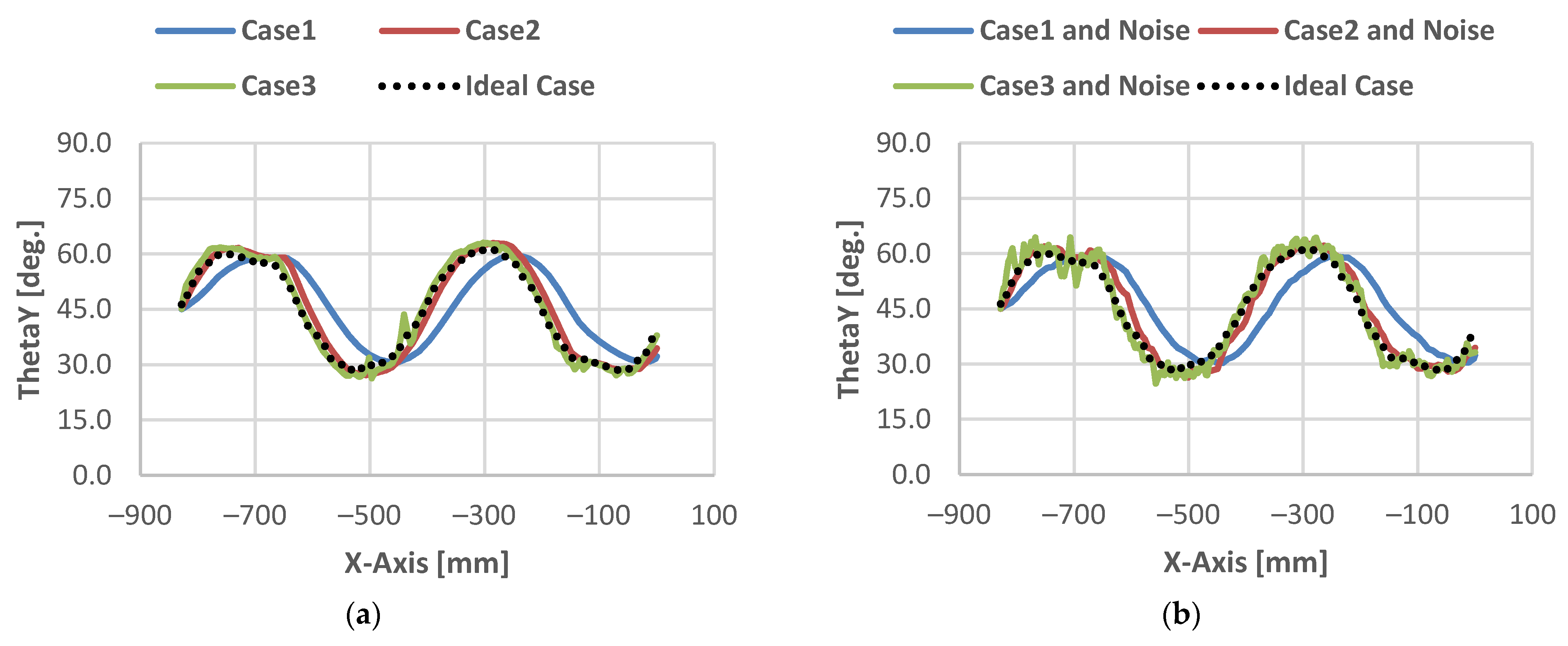
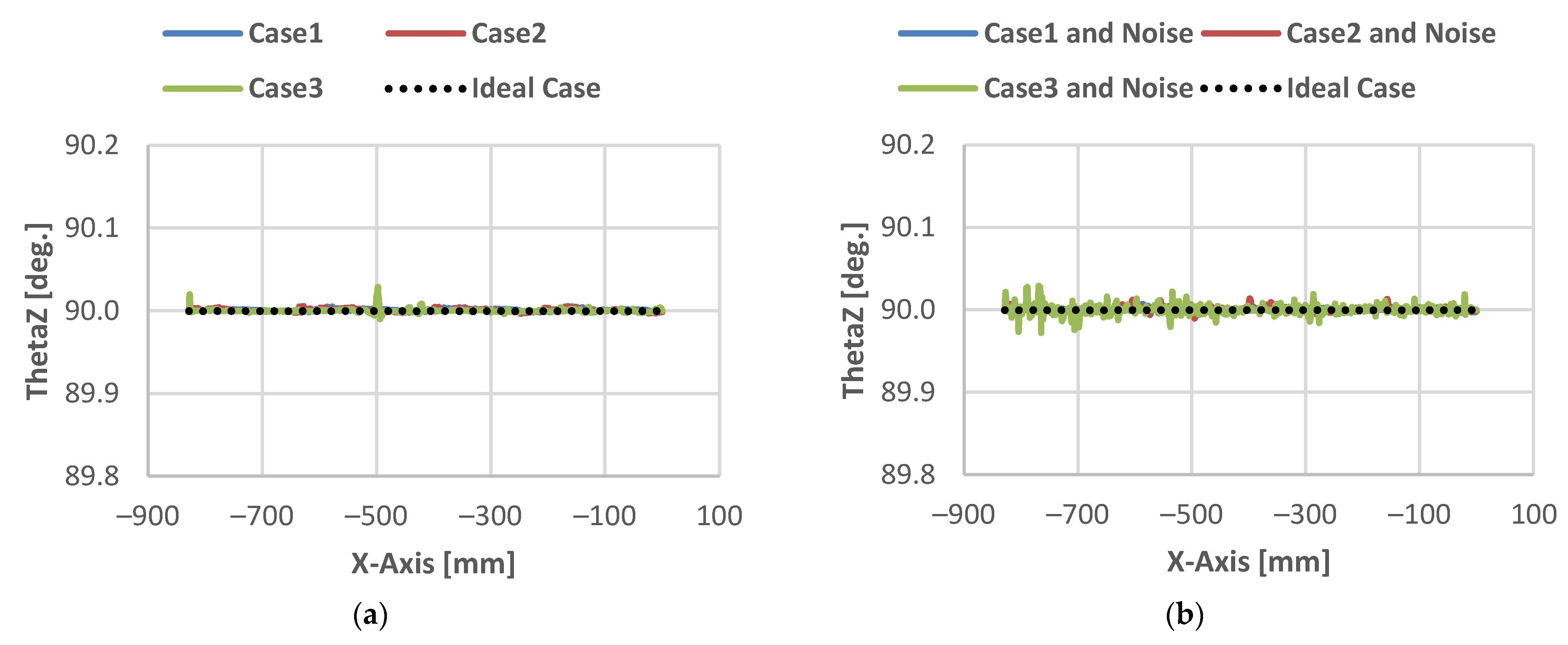
Figure 1. This figure presents adaptive toolpath planning with sparse sensing for an industrial robot to perform non-contact surface processing: (a) Adaptive toolpath planning needs to guide the robot TCP along unknown worksurface variations by maintaining relative tool orientation and alignment, while the tool travels between known start and end tool poses. The end pose or target also serves as the frame of reference. A toolpath must adapt to unknown worksurface variations along the XZ plane of reference frame. l is the diagonal length of the sensor square arrangement, and φ is the sensor inclination angle. (b) A simulation setup involves an industrial robot equipped with end-of-arm distance sensors and a workpiece with unknown surface variations.
Actuators 14 00279 g001
Figure 2. This figure illustrates the vector operations in (2). Note: p n | B n = p = c o n s t a n t .
Actuators 14 00279 g002
Figure 3. This figure demonstrates a tool θ y angle as a pitch angle between the tool XY plane and a sensed worksurface. Likewise, a tool θ x angle can also be identified as a roll angle between the tool XY plane and a sensed worksurface. The sensor inclination angle φ in Figure 1 is 90 ° .
Actuators 14 00279 g003
Figure 4. This figure shows realtime error tracking with linear quadratic regulation for realtime toolpath planning with sparse sensing. Note that p ˙ r e f is a reference tool speed. All reference inputs are in blue. The gains, K s and K B , are obtained via linear quadratic regulation.
Actuators 14 00279 g004
Figure 5. This figure presents an image sequence of the Case 3 simulation: (1) The robot tool is at the start pose; (2) The robot tool departs from the start pose; (3) The robot tool follows the sensed surface and advances toward the end target; (4) The robot tool keeps following the sensed surface and advancing toward the end target.
Actuators 14 00279 g005
Figure 6. Toolpath θ x angles: (a) no sensor noise; (b) added sensor noise.
Actuators 14 00279 g006
Figure 7. Toolpath θ y angles: (a) no sensor noise; (b) added sensor noise.
Actuators 14 00279 g007
Figure 8. Toolpath θ z angles: (a) no sensor noise; (b) added sensor noise.
Actuators 14 00279 g008
Figure 9. Top views of toolpaths: (a) no sensor noise; (b) added sensor noise.
Actuators 14 00279 g009
Figure 10. Side views of toolpaths: (a) no sensor noise; (b) added sensor noise.
Actuators 14 00279 g010
Figure 11. Toolpath TCP errors along the tool z T axis: (a) no sensor noise; (b) added sensor noise. A positive error means the TCP is above the worksurface, and a negative error means the TCP is below the worksurface.
Actuators 14 00279 g011
Figure 12. RMS errors of toolpath orientation errors: (a) no sensor noise; (b) added sensor noise.
Actuators 14 00279 g012
Figure 13. RMS errors of toolpath TCP for the Figure 11 data.
Actuators 14 00279 g013
Figure 14. This figure presents box-and-whisker plots of actual toolpath speeds: (a) angular speeds of toolpath reorientation; (b) linear speeds of toolpath TCP. Each box-and-whisker plot depicts the upper and lower extremes, the upper and lower quartiles, and the median of each dataset.
Actuators 14 00279 g014
Table 1. Experimental cases with customized weight matrices.
Cases Error   State   Weight   Matrix   Q   R 7 × 7 Control   Weight   Matrix   R   R 7 × 7
Case 1: Reaching the known toolpath target is priority. d i a g ( 1 , 1 , 1 , 1 , 10 , 10 , 10 ) d i a g ( 10 , 10 , 10 , 10 , 1 , 1 , 1 )
Case 2: Balancing the Case 1 and Case 3 goals is priority. d i a g ( 10 , 10 , 10 , 10 , 10 , 10 , 10 ) d i a g ( 10 , 10 , 10 , 10 , 10 , 10 , 10 )
Case 3: Following sensed surface variations is priority. d i a g ( 10 , 10 , 10 , 10 , 1 , 1 , 1 ) d i a g ( 1 , 1 , 1 , 1 , 10 , 10 , 10 )
Table 2. Time-invariant gains obtained via linear quadratic regulation for the three cases in Table 1.
Cases Gains   for   Surface   Error   Tracking :   K s Gains   for   Toolpath   Target   Error   Tracking :   K B
Case 1: Reaching the known toolpath target is priority.0.270.92
Case 2: Balancing the Case 1 and Case 3 goals is priority.0.620.62
Case 3: Following sensed surface variations is priority.0.920.27
Disclaimer/Publisher’s Note: The statements, opinions and data contained in all publications are solely those of the individual author(s) and contributor(s) and not of MDPI and/or the editor(s). MDPI and/or the editor(s) disclaim responsibility for any injury to people or property resulting from any ideas, methods, instructions or products referred to in the content.

