
Angle-Based RGN-Enhanced ADRC for PMSM Compressor Speed Regulation Considering Aperiodic and Periodic Disturbances


Abstract
1. Introduction
- An angle-based RGN is employed to enhance the periodic disturbance observation capability of the ESO, offering an improved solution for addressing variations in disturbance frequency while requiring minimal memory resources.
- A detailed convergence and coupling analysis is conducted, and the parameter tuning methodology is also provided.
- Experimental and simulation results demonstrate that, compared to PI, conventional ADRC, and QRC-ADRC, the proposed method achieves superior disturbance rejection in both steady-state and dynamic conditions.
2. Dynamics Models and Disturbance Analysis
2.1. Dynamics Model of PMSM
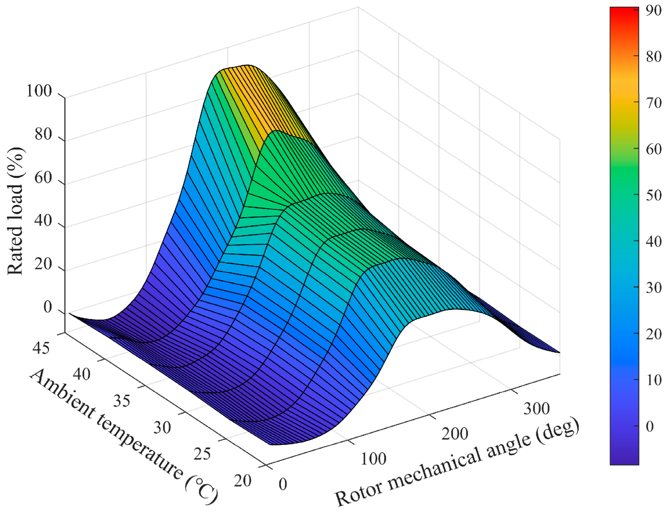
2.2. Disturbance Analysis
- Aperiodic disturbances: These disturbances arise from factors such as parameter mismatches, frictional torque, and non-periodic variations in .
- Periodic disturbances: These disturbances arise from factors such as flux harmonics, inverter nonlinearities, current measurement errors, and periodic variations in . However, among all periodic disturbances, only the first harmonic of is compensated for in this research. This is because, in SRCs, the first harmonic of is dominant, making other periodic disturbances negligible.
3. Proposed Method
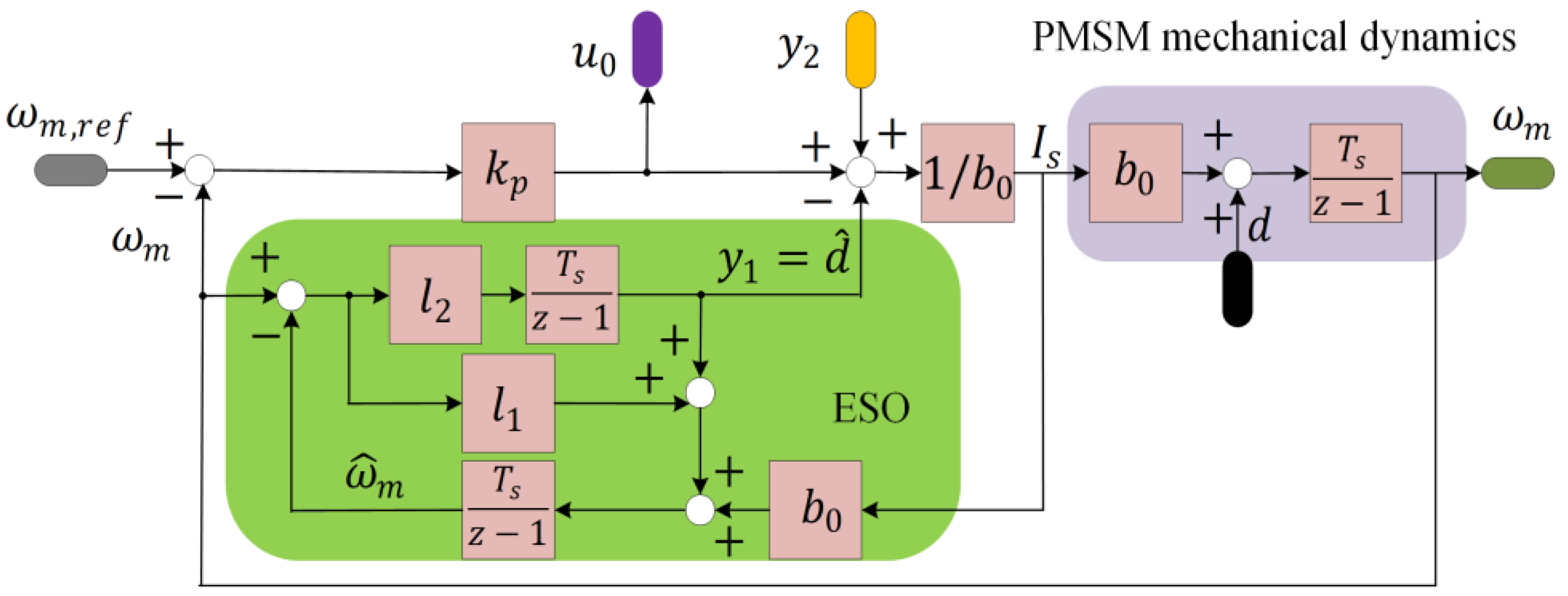
3.1. ADRC
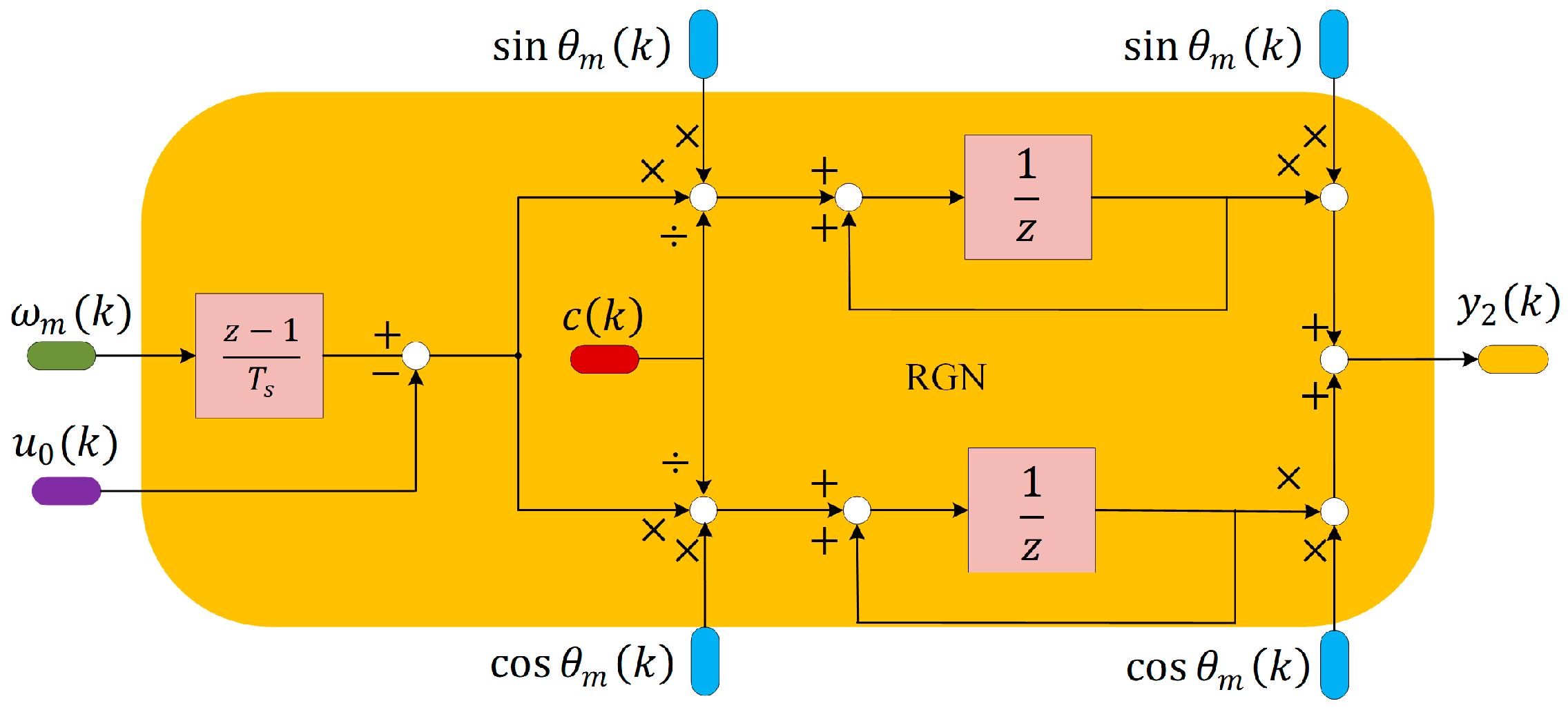
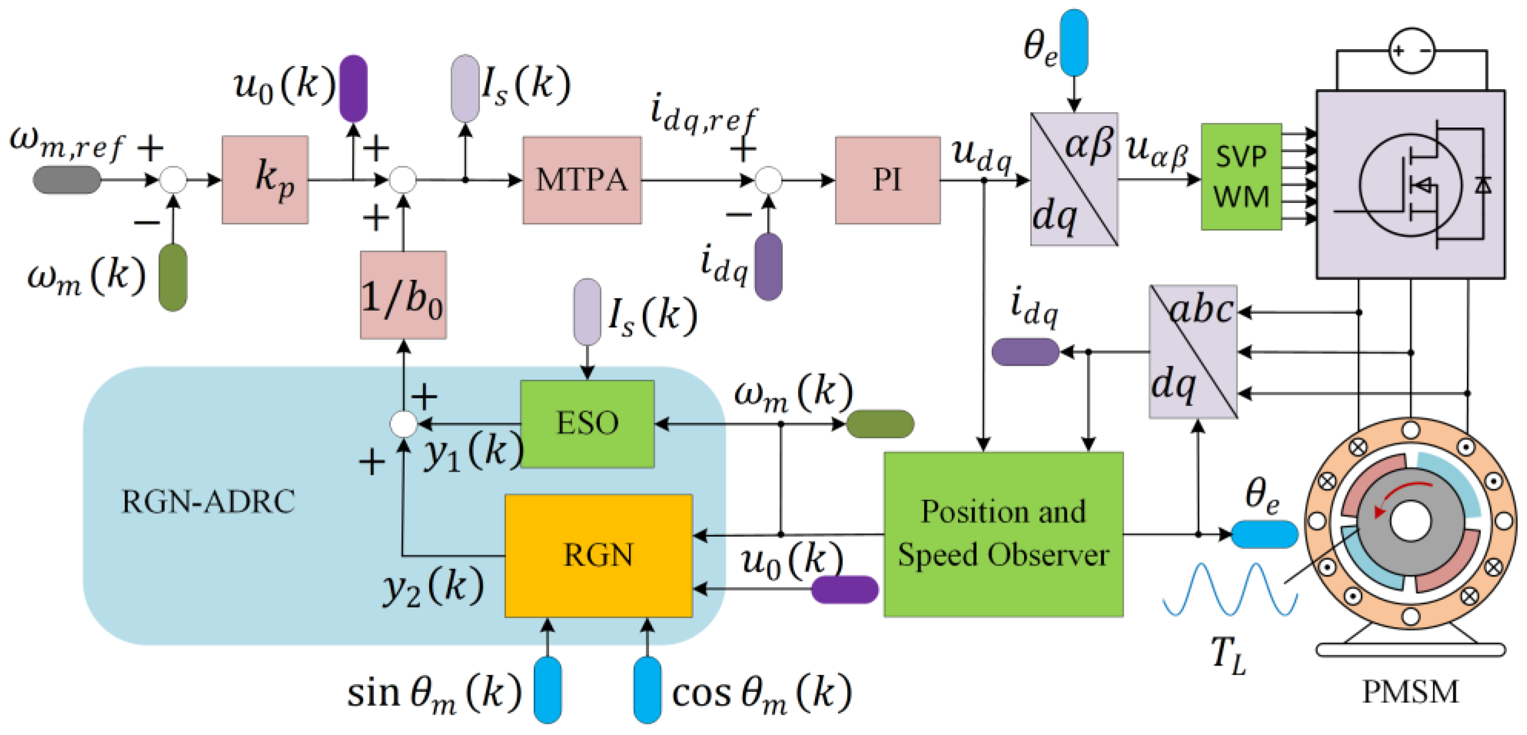
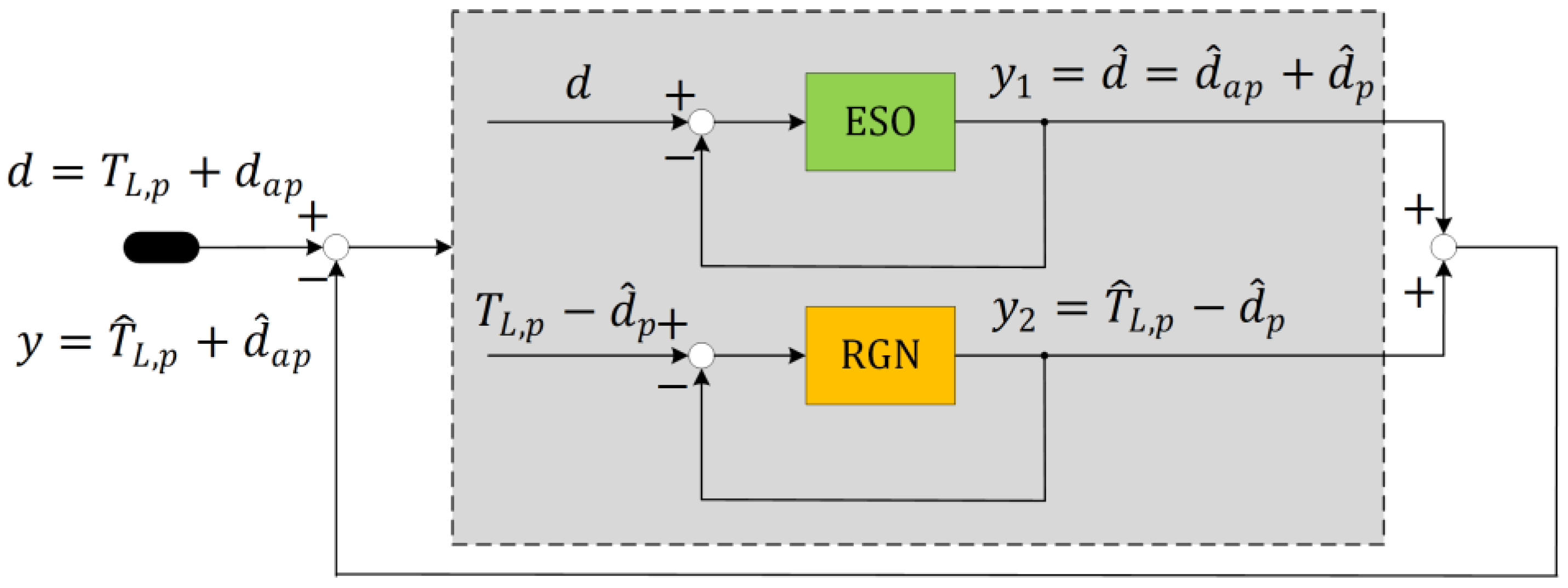
3.2. RGN-ADRC
4. Convergence Analysis
4.1. Convergence Analysis of ESO
4.2. Convergence Analysis of RGN
4.3. Coupling Analysis and Parameter Tuning
5. Experimental Verification
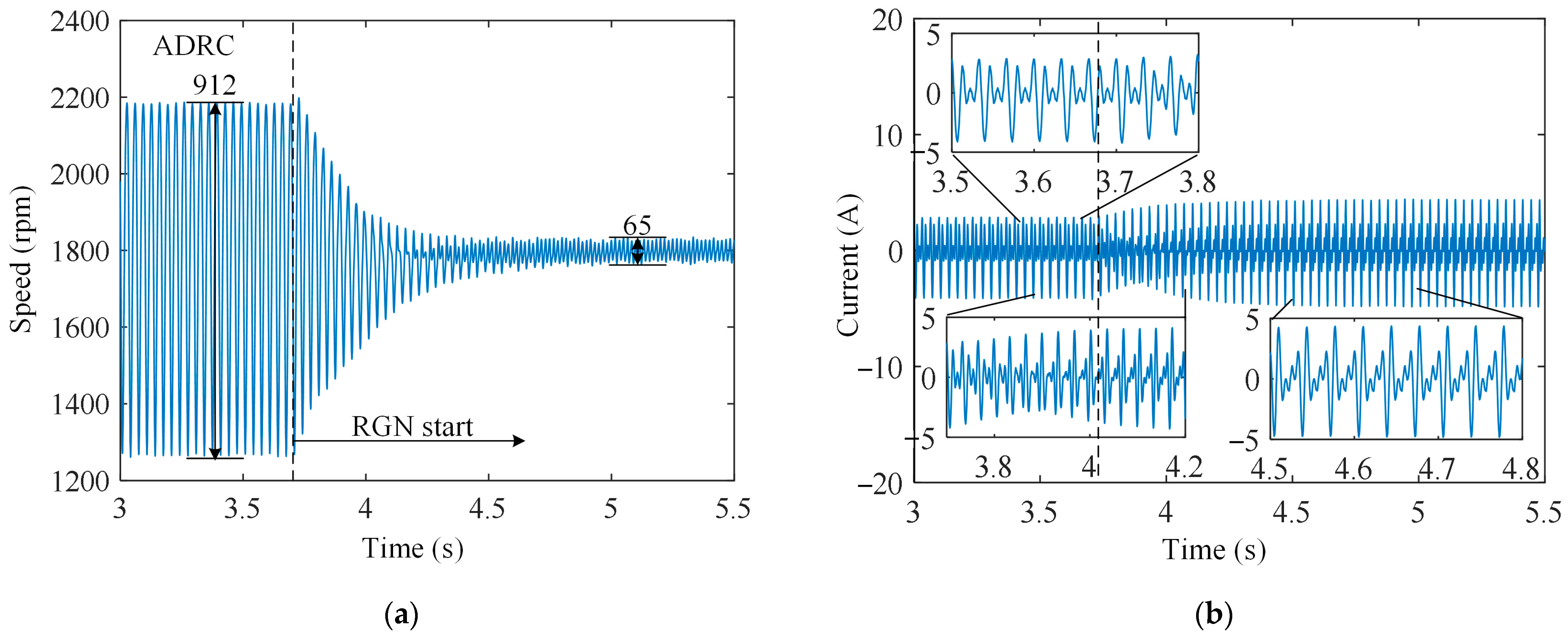
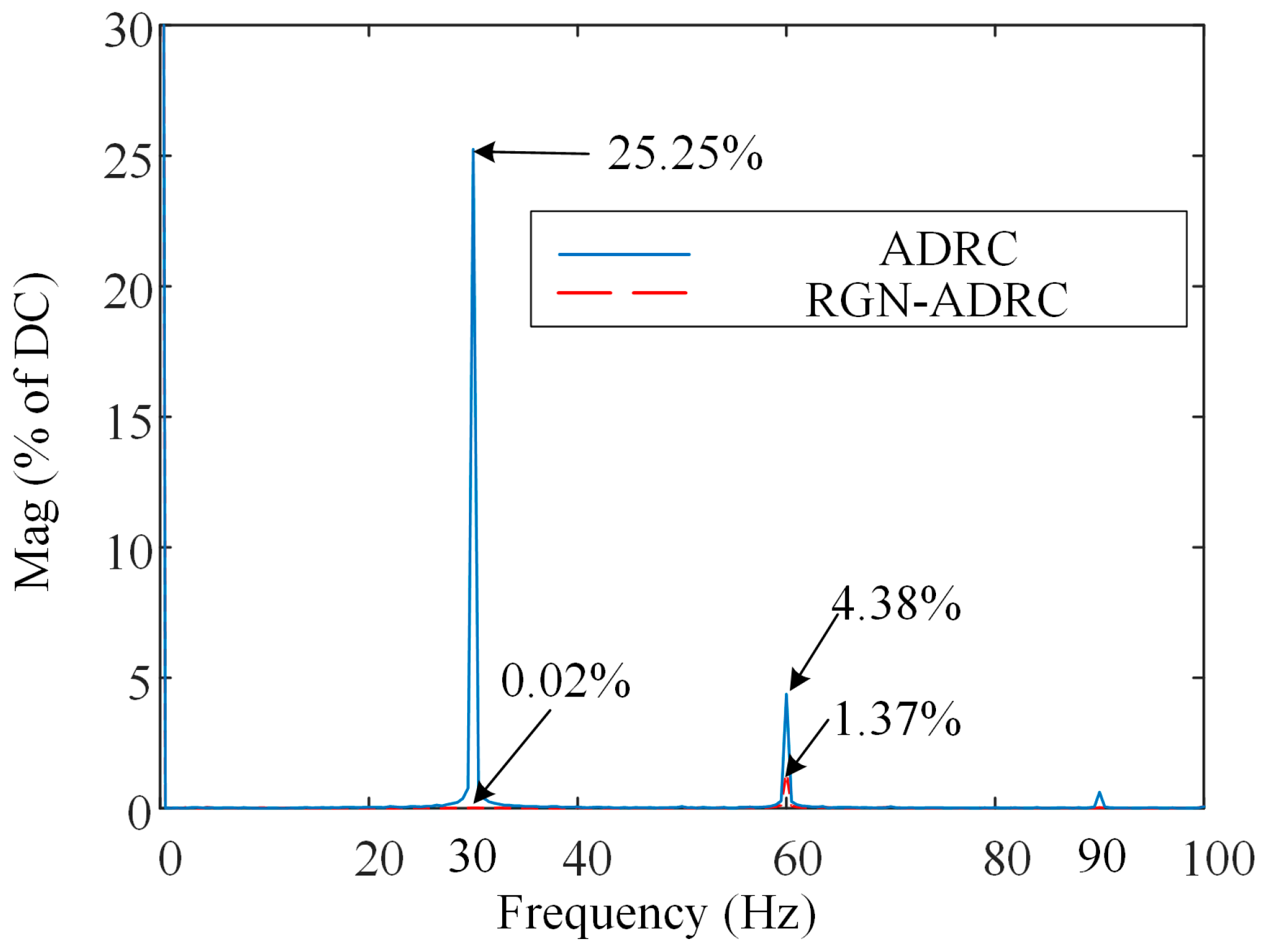
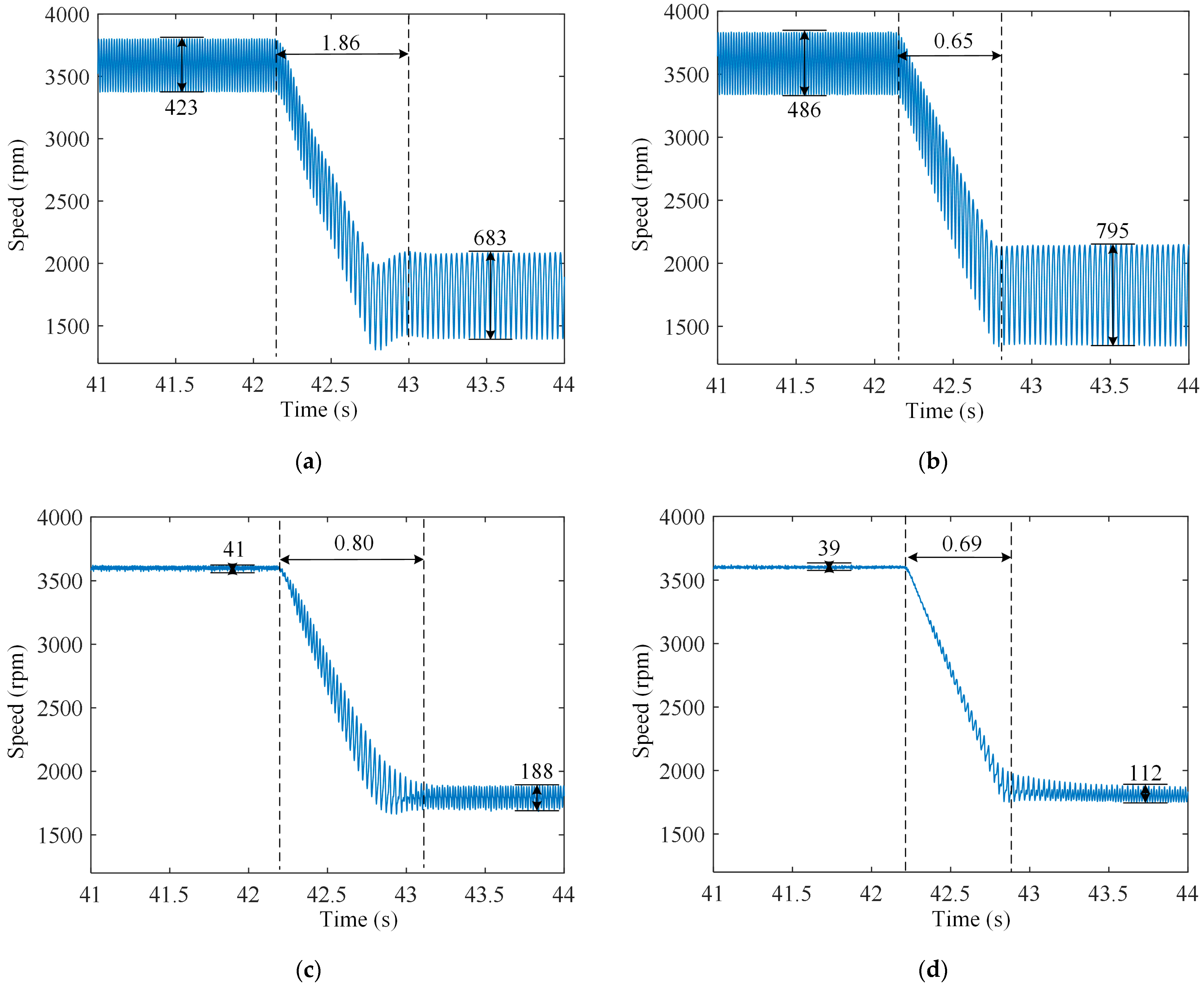
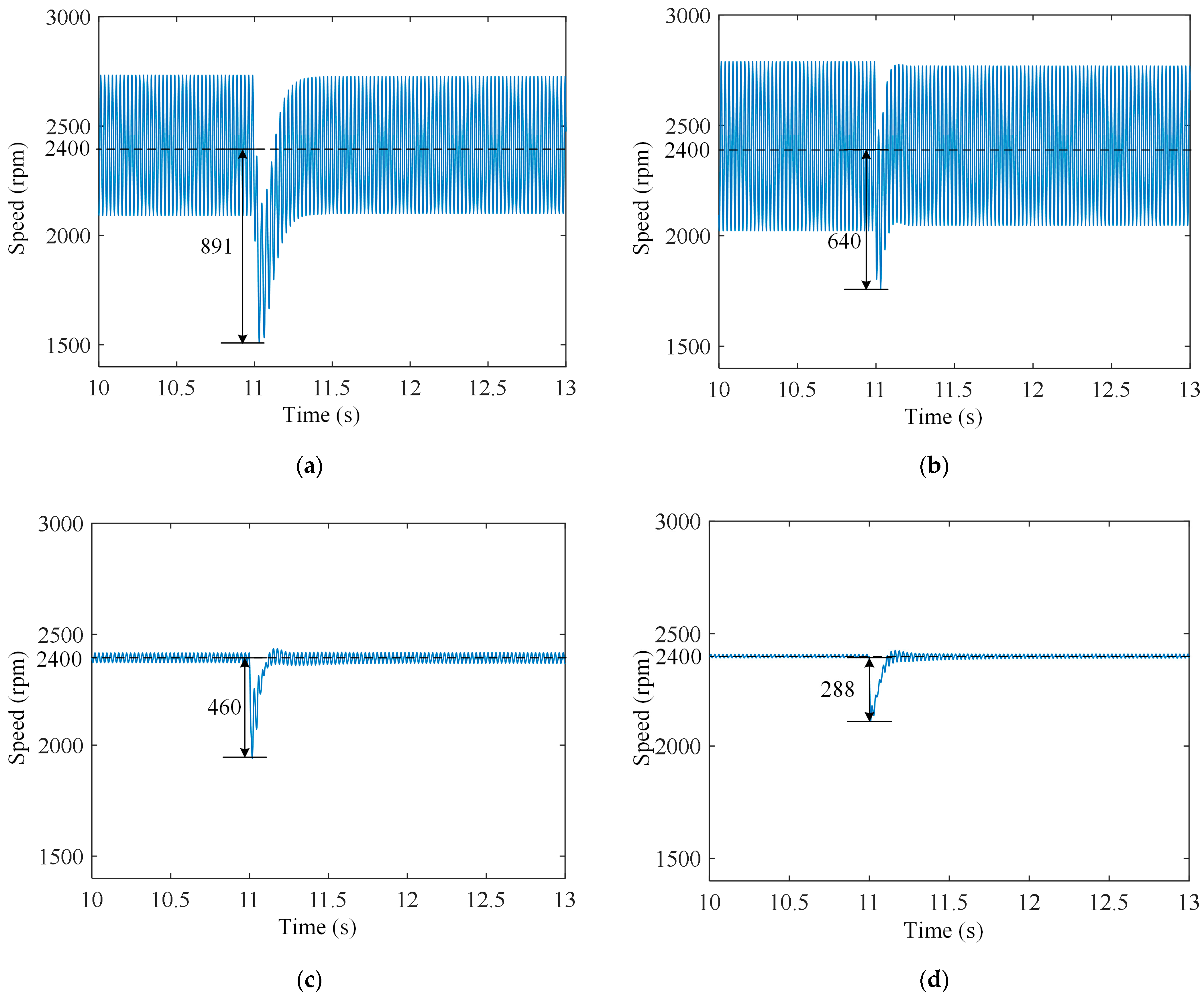
5.1. Disturbance Rejection Performance
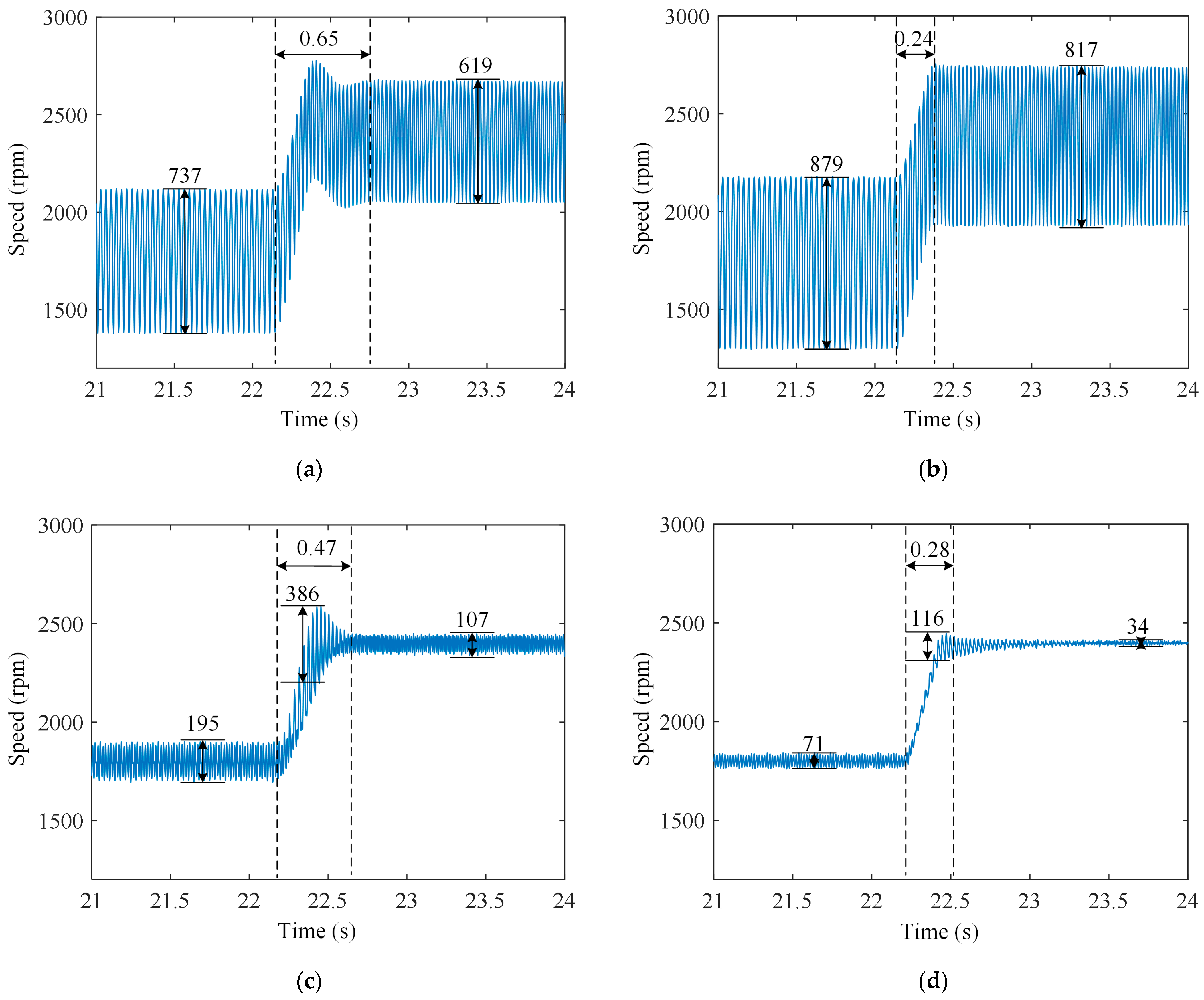
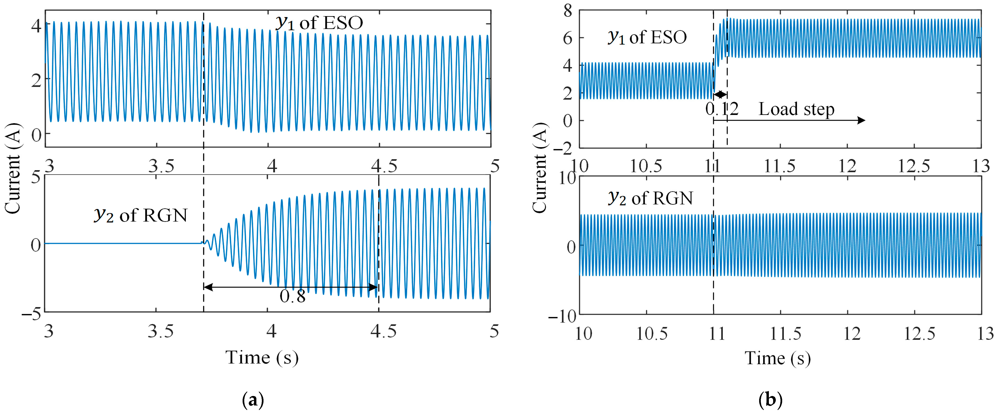
5.2. Decoupling Performance Analysis
6. Conclusions
Author Contributions
Funding
Institutional Review Board Statement
Informed Consent Statement
Data Availability Statement
Conflicts of Interest
References
- Rafaq, M.S.; Jung, J.-W. A Comprehensive Review of State-of-the-Art Parameter Estimation Techniques for Permanent Magnet Synchronous Motors in Wide Speed Range. IEEE Trans. Ind. Inform. 2020, 16, 4747–4758. [Google Scholar] [CrossRef]
- Zhou, Z.; Xia, C.; Yan, Y.; Wang, Z.; Shi, T. Disturbances attenuation of permanent magnet synchronous motor drives using cascaded predictive -integral-resonant controllers. IEEE Trans. Power Electron. 2018, 33, 1514–1527. [Google Scholar] [CrossRef]
- Ahn, H.; Kim, S.; Park, J.; Chung, Y.; Hu, M.; You, K. Adaptive Quick Sliding Mode Reaching Law and Disturbance Observer for Robust PMSM Control Systems. Actuators 2024, 13, 136. [Google Scholar] [CrossRef]
- Hu, B.; Huang, Z. Linear Quadratic Extended State Observer Based Load Torque Compensation for PMSM in a Single Rotor Compressor. In Proceedings of the 2019 22nd International Conference on Electrical Machines and Systems (ICEMS), Harbin, China, 11–14 August 2019; pp. 1–4. [Google Scholar]
- Wang, Y.; Li, P.; Shen, J.-X.; Jiang, C.; Huang, X.; Long, T. Adaptive Periodic Disturbance Observer Based on Fuzzy Logic Compensation for Speed Fluctuation Suppression of PMSM Under Periodic Loads. IEEE Trans. Ind. Appl. 2024, 60, 5751–5762. [Google Scholar] [CrossRef]
- Han, J. From PID to Active Disturbance Rejection Control. IEEE Trans. Ind. Electron. 2009, 56, 900–906. [Google Scholar] [CrossRef]
- Godbole, A.A.; Kolhe, J.P.; Talole, S.E. Performance analysis of generalized extended State observer in tackling sinusoidal disturbances. IEEE Trans. Control Syst. Technol. 2013, 21, 2212–2223. [Google Scholar] [CrossRef]
- Tian, M.; Wang, B.; Yu, Y.; Dong, Q.; Xu, D. Adaptive Active Disturbance Rejection Control for Uncertain Current Ripples Suppression of PMSM Drives. IEEE Trans. Ind. Electron. 2024, 71, 2320–2331. [Google Scholar] [CrossRef]
- Zhu, S.; Huang, W.; Zhao, Y.; Lin, X.; Dong, D.; Jiang, W.; Zhao, Y.; Wu, X. Robust speed control of electrical drives with reduced ripple using adaptive switching high-order extended state observer. IEEE Trans. Power Electron. 2022, 37, 2009–2020. [Google Scholar] [CrossRef]
- Miklosovic, R.; Radke, A.; Gao, Z. Discrete implementation and generalization of the extended state observer. In Proceedings of the 2006 American Control Conference, Minneapolis, MN, USA, 14–16 June 2006; pp. 2209–2214. [Google Scholar]
- Guo, B.; Bacha, S.; Alamir, M.; Hably, A.; Boudinet, C. Generalized integrator-extended state observer with applications to grid-connected converters in the presence of disturbances. IEEE Trans. Control Syst. Technol. 2021, 29, 744–755. [Google Scholar] [CrossRef]
- Zuo, Y.; Zhu, J.; Jiang, W.; Xie, S.; Zhu, X.; Chen, W.-H.; Lee, C.H.T. Active disturbance rejection controller for smooth speed control of electric drives using adaptive generalized integrator extended state observer. IEEE Trans. Power Electron. 2023, 38, 4323–4334. [Google Scholar] [CrossRef]
- Cao, H.; Deng, Y.; Zuo, Y.; Li, H.; Wang, J.; Liu, X.; Lee, C.H.T. Improved ADRC With a Cascade Extended State Observer Based on Quasi-Generalized Integrator for PMSM Current Disturbances Attenuation. IEEE Trans. Transp. Electrif. 2024, 10, 2145–2157. [Google Scholar] [CrossRef]
- Zhuo, S.; Ma, Y.; Liu, X.; Zhang, R.; Jin, S.; Huangfu, Y. Quasi-Resonant-Based ADRC for Bus Voltage Regulation of Hybrid Fuel Cell System. IEEE Trans. Ind. Electron. 2025, 72, 439–448. [Google Scholar] [CrossRef]
- Wang, Z.; Zhao, J.; Wang, L.; Li, M.; Hu, Y. Combined vector resonant and active disturbance rejection control for PMSLM current harmonic suppression. IEEE Trans. Ind. Inform. 2020, 16, 5691–5702. [Google Scholar] [CrossRef]
- Wang, B.; Tian, M.; Yu, Y.; Dong, Q.; Xu, D. Enhanced ADRC with Quasi-Resonant Control for PMSM Speed Regulation Considering Aperiodic and Periodic Disturbances. IEEE Trans. Transp. Electrif. 2022, 8, 3568–3577. [Google Scholar] [CrossRef]
- Wu, H.; Gan, C.; Wang, H.; Wang, S.; Qu, R.; Liu, X. Active Disturbance Rejection Speed Control With Double-Stage-ESO Considering Aperiodic and Periodic Disturbances for PMSM Drives. IEEE Trans. Ind. Electron. 2025; early access. [Google Scholar] [CrossRef]
- Liu, X.; Deng, Y.; Wang, J.; Li, H.; Cao, H. Fixed-time generalized active disturbance rejection with quasi-resonant control for PMSM speed disturbances suppression. IEEE Trans. Power Electron. 2024, 39, 6903–6918. [Google Scholar] [CrossRef]
- Liu, X.; Deng, Y.; Cao, H.; Wang, J.; Li, H.; Lee, C.H.T. Modified ADRC Based on Quasi-Resonant Fixed-Time-Convergent Extended State Observer for PMSM Current Regulation. IEEE Trans. Transp. Electrif. 2025, 11, 1416–1430. [Google Scholar] [CrossRef]
- Tian, M.; Wang, B.; Yu, Y.; Dong, Q.; Xu, D. Discrete-time repetitive control-based ADRC for current loop disturbances suppression of PMSM drives. IEEE Trans. Ind. Informat. 2022, 18, 3138–3149. [Google Scholar] [CrossRef]
- Xu, J.; Wei, Z.; Wang, S. Active Disturbance Rejection Repetitive Control for Current Harmonic Suppression of PMSM. IEEE Trans. Power Electron. 2023, 38, 14423–14437. [Google Scholar] [CrossRef]
- Luo, C.; Xu, Z.; Yang, K.; Li, W.; Huang, Y. Multiple Disturbance Suppression of IPMSM Drives Based on Embedded Discrete-Time Repetitive ADRC With Optimized Parameter Selection. IEEE Trans. Power Electron. 2024, 39, 6052–6062. [Google Scholar] [CrossRef]
- Huang, D.; Min, D.; Jian, Y.; Li, Y. Current-cycle iterative learning control for high-precision position tracking of piezoelectric actuator system via active disturbance rejection control for hysteresis compensation. IEEE Trans. Ind. Electron. 2020, 67, 8680–8690. [Google Scholar] [CrossRef]
- Tian, M.; Wang, B.; Yu, Y.; Dong, Q.; Xu, D. Enhanced One Degree-of-Freedom ADRC With Sampled-Data Iterative Learning Controller for PMSM Uncertain Speed Fluctuations Suppression. IEEE Trans. Transp. Electrif. 2024, 10, 8321–8335. [Google Scholar] [CrossRef]
- Fei, Q.; Deng, Y.; Li, H.; Liu, J.; Shao, M. Speed Ripple Minimization of Permanent Magnet Synchronous Motor Based on Model Predictive and Iterative Learning Controls. IEEE Access 2019, 7, 31791–31800. [Google Scholar] [CrossRef]
- Tang, M.; Formentini, A.; Odhano, S.A.; Zanchetta, P. Torque Ripple Reduction of PMSMs Using a Novel Angle-Based Repetitive Observer. IEEE Trans. Ind. Electron. 2020, 67, 2689–2699. [Google Scholar] [CrossRef]
- Wang, S.; Zhang, G.; Wang, Q.; Ding, D.; Bi, G.; Li, B.; Wang, G.; Xu, D. Torque Disturbance Compensation Method Based on Adaptive Fourier-Transform for Permanent Magnet Compressor Drives. IEEE Trans. Power Electron. 2023, 38, 3612–3623. [Google Scholar] [CrossRef]
- Zhang, C.; Yang, Y.; Gong, Y.; Guo, Y.; Song, H.; Zhang, J. Adaptive Periodic Speed Fluctuation Suppression for Permanent Magnet Compressor Drives. Sensors 2025, 25, 2074. [Google Scholar] [CrossRef]
- Gao, Z. Scaling and bandwidth-parameterization based controller tuning. In Proceedings of the American Control Conference, Denver, CO, USA, 4–6 June 2003; pp. 4989–4996. [Google Scholar]
- Dash, P.K.; Hasan, S. A Fast Recursive Algorithm for the Estimation of Frequency, Amplitude, and Phase of Noisy Sinusoid. IEEE Trans. Power Electron. 2011, 58, 4847–4856. [Google Scholar] [CrossRef]
- Zheng, J.; Lui, K.W.K.; Ma, W.-K.; So, H.C. Two Simplified Recursive Gauss–Newton Algorithms for Direct Amplitude and Phase Tracking of a Real Sinusoid. IEEE Signal Process. Lett. 2007, 14, 972–975. [Google Scholar] [CrossRef]
- Hao, Z.; Tian, Y.; Yang, Y.; Gong, Y.; Hao, Z.; Zhang, J. Sensorless Control Based on the Uncertainty and Disturbance Estimator for IPMSMs With Periodic Loads. IEEE Trans. Ind. Electron. 2023, 70, 5085–5093. [Google Scholar] [CrossRef]


| Symbol | Parameter | Value with Unit |
|---|---|---|
| Rated power | 650 W | |
| Rated voltage | AC 220 V | |
| Number of pole pairs | 3 | |
| Rated rotor speed | 3600 rpm | |
| Minimum speed | 900 rpm | |
| Stator resistance | ||
| d-axis inductance | 13.2 mH | |
| q-axis inductance | 18.5 mH | |
| Inertia constant | 0.000286 kg m2 | |
| Torque constant | 0.6 Nm/A |
| Method | Symbol | Value with Unit |
|---|---|---|
| Execution frequency | 8k Hz | |
| PI | 0.0286 | |
| 43 | ||
| ADRC | 50 | |
| 180 rad/s | ||
| 2000 | ||
| QRC | 200 | |
| 0.0015 | ||
| RGN | 0.96 |
| Speed (rpm) | PI | ADRC | QRC-ADRC | Proposed |
|---|---|---|---|---|
| 1200 | 37.85% | 39.73% | 9.87% | 5.73% |
| 1800 | 20.19% | 25.68% | 4.52% | 1.44% |
| 2400 | 12.58% | 16.49% | 1.74% | 0.31% |
| 3600 | 5.98% | 6.95% | 0.43% | 0.27% |
Disclaimer/Publisher’s Note: The statements, opinions and data contained in all publications are solely those of the individual author(s) and contributor(s) and not of MDPI and/or the editor(s). MDPI and/or the editor(s) disclaim responsibility for any injury to people or property resulting from any ideas, methods, instructions or products referred to in the content. |
© 2025 by the authors. Licensee MDPI, Basel, Switzerland. This article is an open access article distributed under the terms and conditions of the Creative Commons Attribution (CC BY) license (https://creativecommons.org/licenses/by/4.0/).
Share and Cite
Zhang, C.; Yang, Y.; Gong, Y.; Guo, Y.; Song, H.; Zhang, J. Angle-Based RGN-Enhanced ADRC for PMSM Compressor Speed Regulation Considering Aperiodic and Periodic Disturbances. Actuators 2025, 14, 276. https://doi.org/10.3390/act14060276
Zhang C, Yang Y, Gong Y, Guo Y, Song H, Zhang J. Angle-Based RGN-Enhanced ADRC for PMSM Compressor Speed Regulation Considering Aperiodic and Periodic Disturbances. Actuators. 2025; 14(6):276. https://doi.org/10.3390/act14060276
Chicago/Turabian StyleZhang, Chenchen, Yang Yang, Yimin Gong, Yibo Guo, Hongda Song, and Jiannan Zhang. 2025. "Angle-Based RGN-Enhanced ADRC for PMSM Compressor Speed Regulation Considering Aperiodic and Periodic Disturbances" Actuators 14, no. 6: 276. https://doi.org/10.3390/act14060276
APA StyleZhang, C., Yang, Y., Gong, Y., Guo, Y., Song, H., & Zhang, J. (2025). Angle-Based RGN-Enhanced ADRC for PMSM Compressor Speed Regulation Considering Aperiodic and Periodic Disturbances. Actuators, 14(6), 276. https://doi.org/10.3390/act14060276