Abstract
Free-form surface polishing is a key process in precision machining within high-end manufacturing, where optimizing the polishing trajectory directly influences both processing quality and efficiency. Traditional trajectory planning methods for free-form surface polishing in high-curvature regions suffer from issues such as a lack of precision, low trajectory continuity, and inefficiency. This paper proposes an improved trajectory planning method based on curvature characteristics, incorporating dynamic partitioning and boundary smoothing algorithms. These methods dynamically adjust according to surface curvature, enhancing processing efficiency and surface quality. Additionally, a hybrid optimization framework combining a genetic algorithm (GA) and local search (LS) is proposed to address the challenges of balancing global optimization with local fine-tuning in traditional trajectory planning methods. These challenges often result in large errors, low machining efficiency, and unstable surface quality. The method optimizes the overall trajectory distribution through a global search using GA while locally refining the high-curvature regions with LS. This combination improves trajectory uniformity and smoothness, and the results demonstrate significant increases in machining efficiency and accuracy. Finally, the feasibility of the trajectory planning method was verified through motion simulation. This paper also provides a detailed description of the mathematical modeling, algorithm implementation, and simulation analysis of the XY-3-RPS hybrid robot for trajectory optimization, offering both a theoretical foundation and engineering support for its application in free-form surface polishing.
1. Introduction
Freeform surfaces are widely used in modern manufacturing applications, including aerospace, precision instruments, mold and die making, and medical devices [1]. The complex geometry of free-form surfaces makes it challenging for traditional machining methods to achieve high precision and quality, particularly in applications requiring high optical or aerodynamic performance. The polishing accuracy of free-form surfaces is critical, and due to their variable shapes, the machining process must be adapted to different workpieces, which is difficult to achieve efficiently with traditional rigid machine tools [2,3]. Therefore, high-degree-of-freedom robots have become a key development direction for free-form surface polishing, as they can enhance processing quality and productivity through flexible trajectory planning and motion control.
The XY-3-RPS hybrid robot integrates the high rigidity and precision of a parallel mechanism with the large workspace and flexibility of a tandem mechanism, making it well-suited for free-form surface polishing [4,5]. The parallel mechanism offers high structural rigidity, effectively suppressing vibration and errors during machining, improving polishing accuracy, and meeting high-finish machining requirements. The XY platform expands the robot’s workspace, allowing it to cover larger free-form surfaces and enhance machining efficiency.
The design and planning of the polishing trajectory are critical for achieving optimal processing results. For complex surface polishing, the choice of trajectory directly influences the quality of the final surface, with different trajectories yielding significantly varying effects on the polished surface [6]. The most commonly used polishing paths are raster, spiral, and pseudo-random paths. However, these methods make it difficult for the machine to respond in real time due to speed variations between neighboring path points, leading to new path errors and reduced efficiency [7]. Isoparametric, isometric, isocurvature, and zigzag trajectories are also commonly used. Isometric trajectories feature constant spacing and improved polishing uniformity. They are suitable for complex surfaces, helping to avoid the inhomogeneity issues associated with parametric methods. However, they are computationally complex and prone to self-intersection in high-curvature regions [8,9]. Chen et al. [10] proposed a trajectory planning algorithm that accounts for the material removal characteristics. Using Hertz theory, the pressure and velocity distributions in the contact area between the spherical polishing tool and the surface are derived. A material removal model for the polishing process is established, and a numerical solution for the optimal row spacing of adjacent polishing trajectories is provided. Zheng Yuxing [11] proposed a multi-directional polishing motion model for surface polishing integrated with the angle conformal parameterization algorithm to enable trajectory planning on 3D mesh surfaces. Based on the theoretical model of mapping deformation and the polishing process in the angle conformal parameterization algorithm, the parameters of the multi-directional polishing motion model are adjusted to control polishing accuracy.
Equal curvature trajectories are suitable for free-form surfaces with significant curvature variations, requiring high machining accuracy in high-curvature regions. However, they demand high-precision curvature calculations and are computationally expensive. The zigzag trajectory is simple, easy to compute, applicable to most free-form surfaces, and offers a continuous path that avoids sudden tool attitude changes, thereby improving machining stability. However, traditional zigzag trajectory planning in high-curvature regions often results in uneven trajectory density, trajectory mutations, and excessive processing errors, negatively impacting polishing quality. After comprehensive consideration, this paper selects the zigzag trajectory but emphasizes the need for optimization to address issues of uneven trajectory density, trajectory mutations, and excessive processing errors in high-curvature regions.
Currently, free-form surface polishing trajectory optimization methods mainly include rule-based approaches, such as zigzag, spiral, or adaptive trajectory generation. However, these methods lack optimization mechanisms, making them difficult to apply in complex surface processing. Amersdorfer et al. [12] proposed a real-time online trajectory planning technique for robotic free-form surface polishing. The end-effector, consisting of a force-controlled robot hand and additional sensors, offers a flexible automated solution for free-form surface grinding and polishing by utilizing real-time data from tracking sensors rather than relying on CAD data or geometrical models. The second category involves intelligent optimization algorithms, such as genetic algorithm (GA), ant colony optimization (ACO), particle swarm optimization (PSO), and local search (LS), which are used for trajectory optimization. However, these methods are computationally intensive and may suffer from slow convergence. Wang Zesheng et al. [13] proposed an improved elite non-dominated sorting genetic algorithm, which effectively addresses multi-objective trajectory optimization, enhancing both optimization quality and computational efficiency. However, challenges remain in balancing diversity and convergence, handling constraints, and expanding its applicability. Fatima Zahra Baghli et al. [14] employed an ant colony algorithm to solve trajectory planning in complex environments, enabling automatic obstacle avoidance and path optimization. Zhu et al. [15] improved the particle swarm optimization (PSO) algorithm to enhance the accuracy and efficiency of robotic arm trajectory planning, enabling quick identification of optimal trajectories and better adaptation to complex welding environments. However, the PSO algorithm may converge to a local optimum in high-dimensional spaces and is sensitive to parameter selection. Gui Hengde [16] analyzed the machining trajectory and motion when polishing free-form surfaces using a robot. He pointed out that the linear cutting method requires the fewest motion joints, minimizing interference and avoiding mechanism singularity. Theoretical analysis indicates that the linear cutting method performs better than the ring-cutting method in optimizing free-form surface polishing and finishing trajectories. Liu Qinglong [17] established a direct relationship between polishing trajectory and material removal by applying a material removal profile. He optimized planar grating, concentric circle, and aspheric spiral trajectories to address material removal uniformity during the polishing process.
Traditional trajectory planning methods often struggle to balance global optimization and local fine-tuning in free-form surface machining, leading to significant errors, low machining efficiency, and unstable surface quality. Global optimization struggles to handle detailed processing of high-curvature regions, while local adjustment lacks overall path coordination, resulting in poor machining accuracy, error accumulation, and compromised surface quality [18]. To address these issues, more flexible trajectory optimization methods are needed to enhance machining accuracy, improve efficiency, and ensure stable surface quality.
To address the aforementioned issues, this paper proposes an automatic partition trajectory planning method based on improved curvature characteristics. By introducing a dynamic partitioning algorithm, the partitioning strategy is adaptively adjusted according to surface curvature variations, enabling accurate division of regions with different curvatures. This significantly improves the efficiency and surface quality of complex surface processing. To optimize the transition at regional boundaries, a boundary smoothing mechanism is incorporated into the partitioning process, enhancing the continuity of the machining path and trajectory accuracy. Furthermore, trajectory optimization is performed by combining the genetic algorithm (GA) and local search (LS), leveraging the global search capability of GA and the local convergence characteristics of LS. This ensures trajectory feasibility while improving its smoothness and processing accuracy. Finally, the kinematic simulation of the generated trajectories is carried out to provide a theoretical basis and data support for subsequent experimental processing. This paper constructs a highly automated and adaptable machining trajectory planning framework, starting from curvature partitioning, path generation, and trajectory optimization. This method enhances precision control in complex surface machining, reduces reliance on manual experience and rule-based modeling, and facilitates the shift from static rule design to dynamic adaptive optimization in trajectory planning. This has significant theoretical value and engineering application potential.
2. Kinematic Modeling of XY-3-RPS Hybrid Robots
2.1. Structure and Principle of Motion
The XY-3-RPS hybrid robot consists of an XY platform placed horizontally at the lower end and an RPS parallel platform with three degrees of freedom. The XY platform can move in the X and Y directions, represented by movements N and M, respectively. The 3-RPS consists of three RPS mechanisms connected in parallel. A sketch of the XY-3-RPS hybrid robot structure is shown in Figure 1.
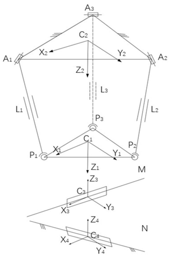
Figure 1.
XY-3-RPS hybrid robot structure sketch.
The following coordinate system is established: the geometric center of the static platform A1A2A3 is taken as the origin of coordinate system C2. X2 points from the geometric center to A1, Y2 is parallel to A3A2, and Z2 is perpendicular to the static platform, directed vertically downward. The geometric center of the moving platform P1P2P3 is taken as the origin of coordinate system C1. X1 points from the geometric center to P1, Y1 is parallel to P3P2, and Z1 is perpendicular to the static platform, directed vertically downward. The coordinate system C3 is established with the geometric center of the Y platform as the origin. X3 is parallel to X2, Y3 is parallel to Y2, and Z3 is perpendicular to the platform, directed vertically upward. The geometric center of the X platform is taken as the origin of the coordinate system C4. X4 is parallel to X2, Y4 is parallel to Y2, and Z4 is perpendicular to the platform, directed vertically upward. The vertical distance between moving sub-M and moving sub-N is 65 mm.
According to the classical Grubler–Kutzbach degrees of freedom equation [19],
where denotes the number of total degrees of freedom of the mechanism; denotes the spatial degrees of freedom; denotes the number of links of the mechanism including the base link; denotes the number of equivalent two-bar joints in the mechanism; denotes the degrees of freedom that joint has.
Since XY-3-RPS is a space mechanism,
After calculation, the mechanism has five degrees of freedom, the XY platform can move along the X and Y directions, the 3-RPS parallel mechanism moves in the Z (vertical) direction, and there is rotational freedom around the X and Y axes. These freedoms meet the requirements for polishing complex surfaces.
2.2. Kinematic Inverse Solution
The rotation matrix of the coordinate system {C1} with respect to {C2} can be expressed by the U-V-W Euler angle representation:
In the above equation, C2RC1 represents the rotation matrix of the coordinate system C1-X1Y1Z1 compared to the coordinate system C2-X2Y2Z2; represents the abbreviation of , represents the abbreviation of , and represents the abbreviation of .
The transformation into a 4 × 4 chi-square transformation matrix is:
In the above equation, C2TC1 denotes the homogeneous transformation matrix of the coordinate system C1-X1Y1Z1 compared to the coordinate system C2-X2Y2Z2; represents the position of the origin of coordinate systems C1-X1Y1Z1 relative to coordinate systems C2-X2Y2Z2.
In the above equation, , , represents the position coordinates of the origin of coordinate systems C1-X1Y1Z1 in coordinate systems C2-X2Y2Z2.
Since the moving platform (P1P2P3) shares a rack with the XY platform, the relationship between the corresponding coordinate systems of the two platforms can be transformed, so the chi-square transformation matrix of the coordinate system {C1} with respect to the coordinate system {C3} is:
In the above equation, C3TC1 denotes the homogeneous transformation matrix of the coordinate system C1-X1Y1Z1 compared to the coordinate system C3-X3Y3Z3, C3TC2 represents the homogeneous transformation matrix of the coordinate system C2-X2Y2Z2 compared to the coordinate system C3-X3Y3Z3.
Due to the orthogonality of the rotation matrix:
Obtainable:
In the above Equation (8):
From the above equation, we can calculate:
The calculation yields Equation (11):
In the above equation, Z24, Z34, and Z12 are all fixed values.
The XY-3-RPS hybrid robot end position inverse solution problem is that is, the problem of determining the inputs (X24, Y34) to each of the parallel active stubs (L1, L2, L3) and XY planar modules (N, M), given the end position parameters (X12, Y12, Z12) and attitude parameters (, , ).
According to the rod length formula of the mixed-link mechanism:
In the above formula, represents the position coordinates of the spherical hinge center in the coordinate system C2-X2Y2Z2, represents the position coordinates of the rotational sub-center in the coordinate system C2-X2Y2Z2, and i takes the values of 1, 2, and 3.
Therefore, by using Equation (12), the position and orientation parameters of the end-effector can be determined, which in turn allows for the calculation of the inputs for each parallel active pivot chain and the tandem planar XY drive module.
3. Free-Form Surface Representation
Among the free-form surface representations, B-spline surfaces offer strong local control, smoothness, and flexibility, making them ideal for complex designs that require fine shape adjustments. NURBS surfaces provide greater flexibility and expressive power but are computationally complex and demanding for designers. Bezier surfaces are simple and intuitive but suffer from poor local control and limited adaptability to complex shapes. High-order polynomial surfaces can fit data accurately but may lead to overfitting and computational instability [20].
The surface roughness of small engine blades, a type of free-form surface, plays a crucial role in their overall performance and service life. A good surface finish can reduce surface stress concentration, prevent fatigue cracks from small defects, and extend blade longevity. Therefore, optimizing surface roughness is critical for small engine blades, which are used here as a representative example of free-form surfaces. In this paper, the selected B-spline surface is used to represent the blade shape, as it allows precise control over the curve and meets complex geometric requirements. Additionally, B-spline surfaces offer better stability and operability in numerical computations, effectively addressing the precision and shape constraints in engine blade design.
A B-spline surface is a smooth surface represented by a linear combination of multiple basis functions, widely used in computer-aided design (CAD) and computer graphics for flexible shape control and high accuracy [21]. A B-spline surface is typically represented by B-spline basis functions in two directions, usually the u and v directions.
Its mathematical expression is:
In the above Equation (13), is the position of the point on the surface, u and v are two parameters, , are determined by the domain of definition of the node vector. are points on the control grid that form a grid. is the ith pth B-spline basis function in the u-direction, defined recursively by the node vector . is the j-th qth B-spline basis function in the v-direction, defined recursively by the node vector .
The B-spline basis function is a segmented polynomial that represents the value of the basis function over a given parameter u. The basis function is a polynomial of the value of the base function. It is usually computed by recursion, satisfying the following conditions:
The basis function is a basis function of order zero, denoted as:
Higher-order basis functions are computed by recursive formulas:
In the above Equation (15), p is the order of the basis function, and ui is an element of the node vector.
4. Automatic Partitioned Trajectory Planning Based on Improved Curvature Properties
4.1. Free-Form Surface Generation
4.1.1. Free-Form Surface Data Acquisition and Processing
The typical method for acquiring free-form surface data involves obtaining the geometric coordinate data of the physical model’s surface using specific measuring equipment and techniques. This process converts the surface geometry into digital data that can be used by CAD/CAM systems.
For subsequent reconstruction of complex surfaces, existing data acquisition methods can be classified into two categories, contact measurement and non-contact measurement, based on their characteristics and applications [22]. Non-contact measurement methods primarily rely on data acquisition principles from optics, acoustics, and related fields, where physical analog quantities are converted into coordinate points on the surface of the measured model using appropriate algorithms. In this study, a non-contact measurement method is employed, with scanning equipment accuracy ranging from 0.1 mm to 1 mm. The point cloud data obtained from professional scanning equipment is shown in Figure 2a.
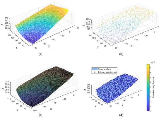
Figure 2.
Surface fitting process and inspection. (a) Raw scanned point cloud data. (b) Preprocessed point cloud data. (c) Fitted B-spline surface. (d) Residual height of the fitted surface from the original point cloud.
Due to factors such as faulty measurement equipment, measurement techniques, and surface shape, measurement data typically suffer from issues such as noise, missing surface data, multiview measurements, distortion, and redundancy [23]. Residual noise can cause minor deviations in the spatial position of point cloud data, leading to fitting errors. Since B-spline surface fitting depends on the accuracy of control points and node vectors, noise can introduce local fluctuations, unevenness, or distortion in the fitted surface, affecting its continuity and smoothness. This not only reduces the geometric accuracy of the surface but can also cause trajectory deviations during tool trajectory planning, which subsequently affects machining accuracy and surface quality. To accurately reconstruct the surface from the measurement data, preprocessing is required, including denoising, simplification, registration, and segmentation, to ensure the quality and continuity of point cloud data. Therefore, it is necessary to preprocess the point cloud data, mainly including point cloud denoising, point cloud simplification, point cloud registration, and point cloud segmentation. The preprocessing of the obtained point cloud data is shown in Figure 2b.
4.1.2. Surface Fitting
After preprocessing the point cloud data, a smooth 3D surface is generated using the B-spline surface fitting method, which serves as the basis for subsequent trajectory generation. B-spline surface fitting creates a smooth 3D surface model by interpolating and fitting the preprocessed point cloud data. The model more accurately represents the spatial distribution of the point cloud, avoiding discontinuities or non-smooth surfaces caused by discretization or noise. By optimizing the control points’ positions, the B-splines provide high smoothness while avoiding overfitting, thus more accurately reflecting the spatial structure of the point cloud [24]. The surface fitted to the processed point cloud data is shown in Figure 2c.
After fitting the B-spline surface, the residual height is an important metric for evaluating the fit quality. The residual height reflects the gap between the fitted surface and the original point cloud data, often used to determine if the surface accurately represents the true structure of the data. Smaller residual heights indicate a better fit, with the fitted surface closely matching the point cloud data. Areas with large residual heights may indicate significant fitting errors in those regions, suggesting that the model needs further optimization or adjustment.
In trajectory planning, large residual heights may impact the accuracy and stability of the paths. Special attention must be given to these regions, adjusting trajectory fineness and path density based on the residual heights to ensure the generated trajectory accurately covers the target surface [25]. Figure 2d shows the resulting plot of the residual height of the fitted surface compared to the original point cloud, with the color of the point cloud mapped according to the residual height.
As can be obtained from Figure 2d, the residual height is close to 0, indicating that the vertical difference between the fitted surface and the original point cloud is minimal. This suggests that the fitted surface accurately represents the original point cloud data, reflecting its spatial structure with minimal error, thereby providing a reliable reference for subsequent trajectory generation and optimization.
4.2. Curvature Calculation
The curvature of a trajectory is a crucial parameter that describes how sharply the trajectory bends. High-curvature regions typically correspond to sharp turns, requiring higher machining accuracy and, therefore, smaller step sizes to maintain the precision of the discrete points along the trajectory. Conversely, low-curvature regions are associated with smoother transitions, allowing for larger step sizes, reducing the number of discrete points, and enhancing machining efficiency [26].
To calculate the trajectory curvature, we first compute it based on the coordinate points along the trajectory using numerical differentiation, applying the following formula:
In the above Equation (16), K is the curvature, and are the coordinates of the trajectory in the two-dimensional plane, respectively, and are the derivatives of the coordinates, and and are the second-order derivatives. The curvature calculation of the fitted surface is shown in Figure 3.
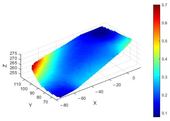
Figure 3.
Curvature distribution graph.
4.3. Automatic Partitioning Based on Improved Curvature Properties
Traditional automatic partitioning methods based on curvature properties typically rely on fixed curvature thresholds. However, this approach suffers from static thresholds, boundary processing issues, and inadequate local adaptation [27]. First, the fixed threshold fails to capture the local variations of the surface, often oversimplifying or excessively refining complex regions. Second, rigid partition boundaries may cause unnatural path transitions, compromising trajectory continuity and machining accuracy. Additionally, the fixed threshold lacks the ability for local adaptation, making it ineffective for regions with sharp curvature changes and preventing dynamic adjustment of trajectory spacing, which undermines overall optimization.
To address these issues, this study presents an automatic partitioning method based on curvature characteristics and introduces a dynamic partitioning algorithm. The method automatically partitions the surface by analyzing its local curvature characteristics in real time, thereby enabling more precise trajectory generation. The following improvements are made:
- (1)
- Curvature-based automatic partitioning
To enhance trajectory adaptability, the method dynamically partitions the surface based on local curvature variations, avoiding reliance on fixed thresholds. Specifically, the curvature at each point is first calculated by analyzing the local curvature of the fitted surface. The curvature variation trend, along with the overall geometric characteristics of the surface, such as curvature distribution, normal variation, and consistency of the principal curvature direction, is used to dynamically partition the surface into multiple regions. Figure 4a shows the schematic diagram of the partition obtained using the fixed partitioning method.
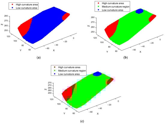
Figure 4.
Automatic partitioning process diagram. (a) Fixed partition schematic; (b) schematic diagram of dynamic partitioning; (c) partition boundary smoothing map.
- (2)
- Dynamic Partitioning Algorithm
During dynamic partitioning, the algorithm adjusts the partition boundary based on changes in local curvature values. In regions with sharp curvature changes, the partition boundary automatically converges to the curvature turning point. In contrast, for regions with gradual changes, the boundary is relaxed to reduce unnecessary distinctions. This approach effectively avoids errors caused by fixed thresholds in traditional methods and allows flexible adjustment according to actual geometric changes. Figure 4b shows the schematic diagram of the partition obtained using the dynamic partitioning method.
The main processes include curvature field calculation, curvature gradient detection, dynamic partition initialization, adaptive region growth, partition merging, and termination. The curvature field calculation involves discrete curvature estimation and normalization. For each vertex , the average curvature is calculated as follows, with the curvature value mapped to the range [0, 1] to avoid dimensional differences:
In the above formula, represents the set of vertices in the 1-ring neighborhood of the vertex , represents the two included angles in the opposite direction of edge , and represents the local area of vertex .
Curvature gradient testing is used to quantify the intensity of curvature changes. For each vertex , its curvature gradient amplitude is calculated by the difference-in-center method:
Normalize the gradient amplitude to the range [0, 1]:
In the initialization of dynamic partitioning, the seeds are selected through curvature extremum detection, and the extremum points that satisfy and have a spacing of are screened. is the average side length.
In adaptive region growth, for partition boundary vertices vi, the growth conditions are:
In the above formula, is taken as the 60% quantile of the curvature gradient distribution, is the curvature difference threshold.
During partition merging, the conditions for merging are:
In the above formula, represents the total number of vertices in the grid, indicates the number of vertices contained in partition .
The termination condition is met when the area change rate is less than 1%, three consecutive iterations occur, or the number of iterations exceeds 100.
- (3)
- Partition Boundary Smoothing
To further enhance partitioning accuracy and trajectory smoothness, this study proposes a partition boundary smoothing technique. In traditional methods, partition boundaries are often rigidly defined, causing abrupt transitions between high and low curvature regions, which affects trajectory continuity and smoothness. Therefore, we introduce a smoothing algorithm to soften the partition boundaries, making transitions between regions more natural and smooth and avoiding discontinuities and computational errors from rigid boundaries. Figure 4c shows the schematic diagram of the partition after the smoothing process.
The partition boundary smoothing process involves boundary neighborhood identification and the design of a weighted smoothing function. After the initial division of the region based on curvature, the boundary point set B is extracted for adjacent high and low curvature regions. A buffer zone width δ is set to extend a transition area on both sides of the boundary, forming a boundary transition zone T. This area satisfies the following condition:
In the above equation, q represents a point in the point cloud, P is the set of points in the point cloud, and (q, B) denotes the shortest Euclidean distance from point q to the boundary point set B.
To ensure a continuous transition of the normal vector, curvature, tangent vector, and other quantities, a distance-based weighting function is introduced in the transition region T. For any point q, the minimum distance to the high curvature region H and low curvature region L is calculated, and the following weight function is constructed:
In the above equation, σ is a smoothing control parameter that adjusts the steepness of the weight transition. The attribute value of the final point q is calculated using the weighted fusion method:
In the above equation, and represent the property estimates of point q in the region of high and low curvature, respectively.
By analyzing and comparing the fixed partition method with the automatic partition method based on curvature characteristics, the Jaccard index is calculated as 0.5632, with the result shown in Figure 5.
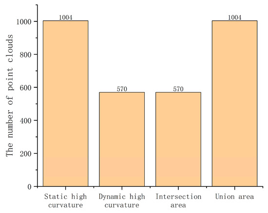
Figure 5.
Point comparison.
The comparative analysis demonstrates that the dynamic high-curvature partitioning method offers significant advantages over the fixed partitioning method. The automatic partitioning method based on curvature characteristics accurately identified 570 core feature points, which were fully included in the detection results of the fixed partitioning method (1005 points) and effectively eliminated 43.7% of misdirected points in the transition zone through intelligent screening. This method demonstrates outstanding feature recognition reliability in precise detection scenarios, such as aero engine blades. This adaptive characteristic makes it an ideal choice for high-precision industrial inspection, while the fixed method is only suitable for initial inspection scenarios that prioritize high detection speed.
In summary, compared to the traditional fixed-threshold partitioning method, the automatic partitioning method based on curvature characteristics offers the following advantages: Higher adaptability: The dynamic partitioning algorithm adjusts the partitioning strategy in real time based on local surface changes, overcoming the limitations of fixed thresholds and refining trajectory generation. Smoother transitions: Boundary smoothing ensures a more natural transition between high- and low-curvature areas, reducing trajectory discontinuity caused by rigid partition boundaries. Optimized trajectory accuracy: This method uses smaller steps in high-curvature areas and larger steps in low-curvature areas, generating a trajectory path adapted to different surface features more efficiently while ensuring both accuracy and computational efficiency.
4.4. Extraction of Effective Polishing Areas
The surface of the leaf body cannot be fully machined due to complex geometrical structures on the blade and the significant influence of the tool size on machining accuracy. Tools are prone to interference near the leaf root, and edge effects occur when machining the blade’s edges, adversely affecting subsequent operations [28]. This paper extracts the effective polishing area by calculating the safety pitch based on the tool’s geometrical characteristics and the blade’s structural features to avoid polishing head interference and blade edge effects.
When extracting the effective polishing region of the blade, safe spacing must be determined in both the length and width directions to avoid tool interference and ensure the stability of the machining process. First, in the length direction of the blade, the entire leaf root or leaf back region is selected, and the parameter range in the uuu-direction is extracted. Assuming that the blade extends along the uuu-direction, a safe spacing must be set to prevent tool interference in the leaf root region. Assuming that the maximum contour radius of the cemented abrasive tool is Rmax and the safety margin is d1, the safety pitch L1 is calculated as:
As shown in Figure 6, based on the calculated safety spacing L1, the boundary positions of the effective region are determined and labeled as b1 and b2. The corresponding u-direction parameter values, u1 and u2, are then extracted to specify the u-direction range of the effective polishing region.
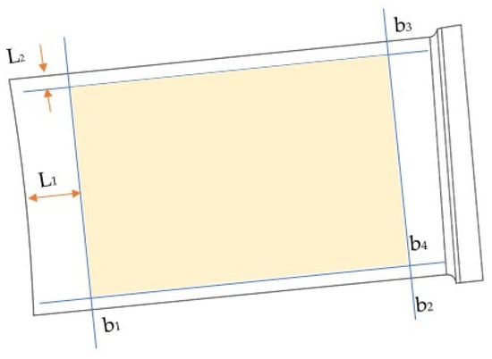
Figure 6.
Effectively polished areas.
In the width direction of the blade, to prevent tool interference in the edge region, the safety spacing must be further determined. Assuming that the minimum distance between the centerline of the cemented abrasive tool and the edge of the blade is ds and setting the safety margin to d2, the safety spacing L2 in the width direction is:
As shown in Figure 6, based on the calculated safety spacing L2, the boundary locations of the effective region are determined and labeled as b3 and b4. The corresponding v-direction parameter values, v1 and v2, are then extracted to specify the v-direction range of the effective polished region.
4.5. Trajectory Generation
The core objective of the trajectory generation module is to create scanning paths that cover the entire surface. To ensure uniform coverage and smooth paths, a zigzag scanning method is used, scanning the surface line by line. This method is particularly suitable for machining small engine blades, ensuring uniform path distribution while avoiding gaps or excessive repetitions, thereby improving machining efficiency [29,30]. Engine blades often have complex geometries, and the zigzag trajectory can adapt to surface irregularities, preventing overly dense or sparse paths while ensuring uniform coverage and guaranteeing machining continuity and accuracy. The trajectory generated by the zigzag method is shown in Figure 7.
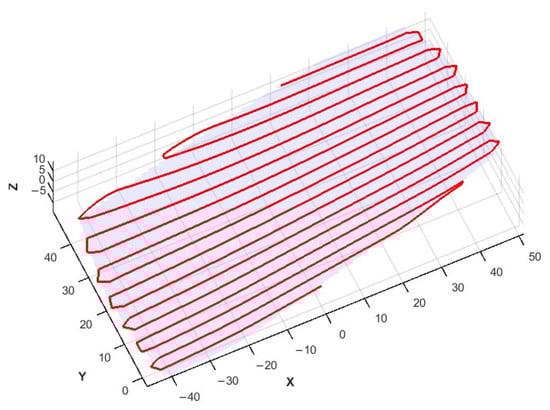
Figure 7.
Three-dimensional display of the original trajectory.
Overall, the zigzag trajectory generation effectively covers the entire surface and ensures smoothness and accuracy during the machining process. By incorporating dynamic step adjustment of curvature, trajectory generation ensures both the precision of the machining path and optimized computational efficiency. This method is especially suitable for precision workpieces with complex curves, such as small engine blades, meeting the demand for high-precision machining and improving efficiency.
4.6. Tool Site Generation
In precision machining, trajectory discretization and interpolation are key to achieving high precision. To improve machining efficiency and accuracy, the discrete interpolation method must incorporate curvature information and adaptively adjust step size, particularly in regions with large curvature changes. In this paper, the discretization of the trajectories is carried out for the already optimized trajectories.
During trajectory discretization, step size selection directly affects the number of discrete points and trajectory accuracy. To accommodate the requirements of varying curvature regions, we employ a dynamic interpolation method. Based on the calculated curvature values, we assign a suitable step size to each segment and calculate the corresponding points via interpolation. This dynamic step interpolation method allows finer control of trajectory discretization, avoids excessive interpolation points in unnecessary areas, and ensures sufficient discrete points in critical high-curvature regions, thus improving both accuracy and efficiency. The optimized trajectory is discretized, and the results are obtained and shown in Figure 8.
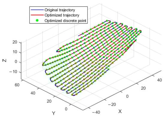
Figure 8.
Schematic diagram of processing contacts.
By combining trajectory curvature information and dynamically adjusting the step size, the proposed discrete interpolation method improves machining efficiency while ensuring trajectory accuracy. This method uses a smaller step size in high-curvature regions and a larger step size in low-curvature regions, effectively considering trajectory characteristics and providing an efficient discretization scheme for precision machining. This dynamic adjustment ensures trajectory accuracy while avoiding excessively dense interpolation points in flat areas, thereby improving processing efficiency. Future research can further optimize the step size strategy to accommodate more complex trajectory shapes and processing requirements.
5. Trajectory Optimization
5.1. Trajectory Optimization Objectives and Strategies
Trajectory optimization is central to the planning process, aiming to improve path quality while ensuring the trajectory satisfies machining constraints and achieves an optimal balance of path length and smoothness [31]. To achieve this, the study combines genetic algorithm (GA) and local search (LS), using GA’s selection, crossover, and mutation operations for global trajectory search, while LS further refines the optimized path.
5.1.1. Trajectory Optimization Objective Definition
The goal of trajectory optimization is to evaluate and enhance trajectory performance based on various criteria. The specific objectives are defined by the following functions:
- (1)
- Trajectory Smoothness
Trajectory smoothness seeks to minimize curvature variations between trajectory points, ensuring machining stability. During machining, curvature variations can cause excessive force fluctuations or machine vibrations, affecting machining quality.
- (2)
- Total trajectory length
Total trajectory length is the cumulative distance between all trajectory points. Longer trajectories increase machining time and energy consumption, so trajectory length should be minimized.
- (3)
- Machining error
Machining error is the height difference between trajectory points and the target surface. The smaller the height difference, the higher the machining accuracy. The goal is to ensure that trajectory points are as close as possible to the target surface.
5.1.2. Optimization Objective Function Definition
The trajectory optimization objective function can incorporate the following metrics: curvature smoothness, which minimizes sudden curvature changes to ensure trajectory smoothness. Trajectory length, which minimizes total trajectory length. Machining error, which ensures trajectory points are close to the target surface and minimizes height error.
The objective function f can be expressed as:
In Equation (12), is the curvature of the ith trajectory point; is the distance between neighboring trajectory points; is the height of the ith trajectory point, is the height of the target surface; is the weight coefficients, which are used for balancing different optimization objectives.
In multi-objective trajectory optimization, each evaluation metric typically has different physical dimensions and numerical ranges. Without normalization, the direct weighted summation may cause metrics with larger numerical scales to dominate the optimization, masking the influence of other metrics and introducing bias into the results. To ensure fairness and comparability of each metric in the objective function, it is essential to normalize them to the same order of magnitude, thereby enhancing the stability and accuracy of multi-objective optimization.
This paper employs the maximum normalization method to standardize the multi-indicator objective function in path optimization. The normalized objective function enhances numerical stability and optimization fairness, providing a reliable basis for multi-objective weight control and effectively addressing the imbalance of multi-dimensional objective functions.
Each indicator is divided by its maximum possible value, typically the theoretical or empirical maximum, to standardize its range to [0, 1]:
Normalization factor for curvature change term:
Path length term normalization factor:
Normalization factor of machining error term:
The objective function after using the maximum normalization method is:
After applying the maximum normalization method, the values of the three components in the objective function are all within the range of 0 to 1, ensuring that the contribution of each component is not biased by differences in order of magnitude.
5.2. Genetic Algorithm (GA) Optimization
The genetic algorithm (GA) is a global search method commonly used for optimization problems. Figure 9 illustrates the detailed steps of the GA applied to the trajectory optimization task.
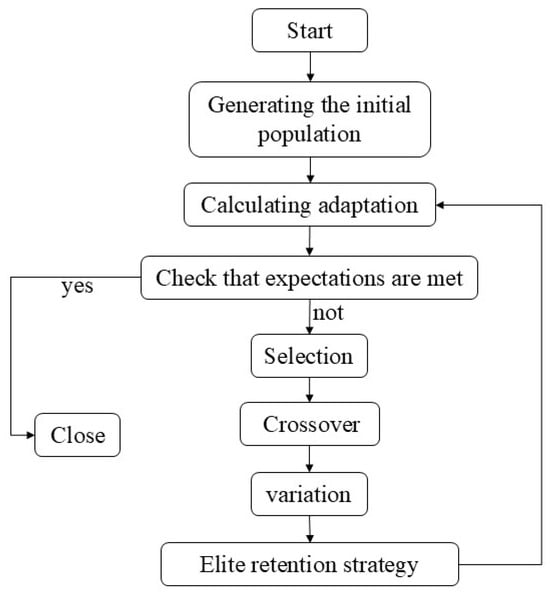
Figure 9.
Genetic algorithm flowchart.
The population is initialized, and the track points are represented by real numbers, with each individual containing a set of coordinates for these points. The coordinates of each trajectory point are represented by and are generated in conjunction with surface normal vector constraints. In the adaptation assessment, the objective function includes the smoothness, total length, and error of the trajectory, and the weighting factor can be adjusted according to the actual needs. The objective function value for each individual is evaluated to assess the performance of each trajectory. Selection proceeds by choosing better-adapted individuals for the next generation through a tournament strategy. Tournament selection improves the survival probability of well-adapted individuals by randomly selecting a group and retaining the best ones. Crossover operation, which generates a new generation of individuals through a two-point crossover operation. This operation exchanges the genetic information of two-parent individuals, producing offspring with greater diversity. The variation operation increases the diversity of trajectory points by adding Gaussian noise near the points. In high-curvature regions, the mutation rate is increased to enhance search capability and avoid local optima. The elite retention strategy ensures that optimal solutions are preserved during crossover and mutation by retaining the best individuals from each generation. The key parameters of the genetic algorithm in this paper are set as follows: population size is 80, crossover rate is 0.9, mutation rate is 0.02, maximum iteration is 300, and elite retention rate is 10%.
5.3. Local Search (LS) Optimization
The local search focuses on refining the initial solution obtained by the GA to enhance the smoothness and accuracy of the trajectory. Figure 10 illustrates the specific process steps of the local search (LS) for the trajectory optimization task.
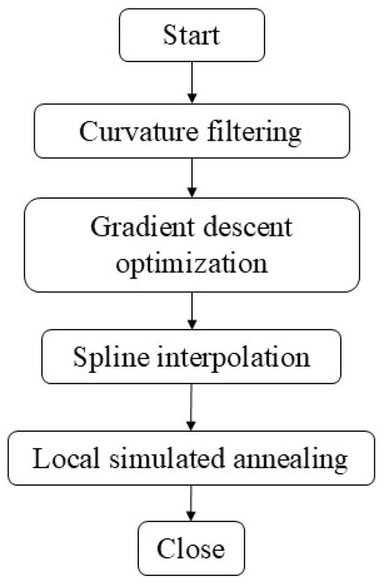
Figure 10.
Local search flowchart.
Curvature filtering calculates the curvature of the trajectory and removes areas with high curvature. These areas typically indicate regions of the trajectory that require further optimization. Gradient descent optimization uses the gradient descent method to minimize the error between the trajectory and the target surface. This method reduces the error by adjusting the trajectory points along the gradient direction of the error. Spline interpolation uses B-spline methods to smooth the trajectory, improving its smoothness and avoiding discontinuities or abrupt changes. The key parameters of the local search algorithm are as follows: LS is triggered every 5 generations, with a neighborhood search depth of 25 iterations.
In the local search phase, this paper adopts the following strategies to enhance global search and prevent premature convergence. First, the initial LS solution is not randomly generated but selected from a set of better individuals obtained by the genetic algorithm, providing a more representative starting point. Second, a moderate perturbation mechanism is introduced in the local search, automatically applying a perturbation near the current solution when the search stagnates or fitness improvement is insufficient over several generations, helping to escape local extrema. Additionally, in high-curvature regions, we dynamically adjust the step size and convergence threshold of the local search based on curvature estimation, preventing the algorithm from overlooking potential optimal solutions due to excessive convergence speed.
5.4. GA + LS Combined Strategy
By combining GA and LS optimization methods, the solution quality is further improved through local optimization while retaining global search capability. Figure 11 illustrates the specific process steps of combining the GA and LS optimization methods.
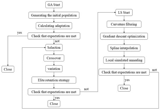
Figure 11.
GA in conjunction with LS flowchart.
GA performs a global search through selection, crossover, and mutation, identifying potentially optimal solutions within a large search space. For the trajectory output by GA, LS optimization further enhances its smoothness and reduces variation in high-curvature regions, resulting in a smoother final trajectory. If the objective function can still be improved after LS, the process returns to GA for secondary optimization. This enables iterations between global and local optimization to achieve a higher-quality solution. The final output, after GA and LS optimization, is the optimal trajectory solution. This trajectory will exhibit high smoothness, minimal overall length, and reduced machining error, meeting the requirements for machining efficiency and accuracy. Figure 12 illustrates the trajectory resulting from the combination of GA and LS optimization methods.
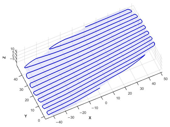
Figure 12.
Optimized 3D display of trajectories.
5.5. Trajectory Comparison and Optimization Effect Analysis
The optimized trajectory is compared with the original to evaluate the optimization effect. The optimization effect was quantified by calculating the total length, average curvature, maximum curvature, speed overrun times, angle overrun times, and other path-related metrics, as shown in Table 1. The results demonstrate a significant improvement in the optimized trajectory, including reduced path length, smoother curvature, and better adherence to constraint conditions.

Table 1.
Trajectory optimization comparison report.
6. XY-3-RPS Hybrid Robot Construction and Simulation
The construction and simulation process of the XY-3-RPS hybrid robot includes multiple stages, such as mechanical structure design, kinematic modeling, control system development, and simulation analysis. The structural design and kinematic modeling have been completed, with the primary focus now on control system development and simulation analysis. The robot’s automatic polishing process ensures proper contact between the polishing tool and the workpiece by controlling the movement of each robot pair according to the predetermined trajectory. First, based on the tool position data on the workpiece surface, the displacement of each moving pair is calculated using the robot kinematic model and then converted into the corresponding motion trajectory. Next, 3D simulation technology is used to verify the polishing trajectory, assess the reasonableness of the pose, and check for any interference during movement. Finally, a polishing program file is generated, meeting the robot control system’s requirements to guide the actual machining operation.
6.1. XY-3-RPS Hybrid Robot Construction
6.1.1. XY-3-RPS Hybrid Robot Control System Design
The XY-3-RPS hybrid robot control system consists of a human–computer interface, GSN motion control card, motor, servo drive, encoders, sensors, scales, and other hardware devices, and completes trajectory planning and motion control tasks using the corresponding application software. During system operation, the computer and motion controller collaborate to generate position and speed commands, driving the motor and mechanical components for precise movements. Simultaneously, the system receives real-time feedback from the components and processes the status information to ensure movement accuracy and stability. Thus, the performance of the hardware directly impacts task execution, processing accuracy, and system stability. Therefore, selecting high-speed, high-precision, stable, and reliable hardware is crucial for determining the overall performance and accuracy of the system.
The XY-3-RPS hybrid robot control system employs the closed-loop control method depicted in Figure 13. The encoder provides speed feedback to adjust motor speed in real time, ensuring movement stability. The scale, installed on the support frame of the linear axis, directly detects the platform’s actual displacement, providing the necessary hardware for the closed-loop system.
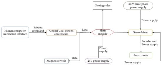
Figure 13.
Schematic diagram of information transmission.
The hardware control system described in this paper primarily includes a human–machine interface, Goodco GSN-024-VT-00 motion control card, axis module, Siemens V90 servo drive, Siemens servo motor, Panasonic A6 servo drive, Panasonic servo motor, among others. The specific hardware connection diagram is shown in Figure 14.
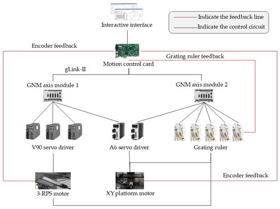
Figure 14.
Hardware platform connection diagram.
6.1.2. XY-3-RPS Mixed-Link Robot Installation
The construction process of the robot platform involves selecting and assembling the hardware system and integrating the electronic control system. After assembling the mechanical system, which includes core components, such as motors, electric cylinders, moving platforms, PCs, and GSN motion control cards, as well as the electronic control system consisting of axis modules, 24 V switching power supplies, servo drives, air switches, and leakage protectors, the construction of the XY-3-RPS hybrid robot is completed. The integration of the mechanical system and electronic control system ensures high efficiency, stable operation, and the ability to meet the stringent requirements of precision, response speed, and stability in the polishing process. The physical construction of the XY-3-RPS hybrid robot is depicted in Figure 15.
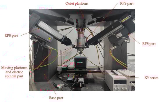
Figure 15.
XY-3-RPS mixed-link robot physical drawing.
6.2. Polishing Simulation Design
In this paper, the XY-3-RPS hybrid robot is modeled using NX12.0 software. To facilitate machining simulation, the robot is divided into several parts: the base, static platform, 3-RPS mechanism, XY platform, and movable platform with electrospindle. A coordinate system consistent with the robot’s motion model is selected. The workpiece coordinate system is then combined with the robot’s coordinate system to accurately describe the relative positions of the end-effector and workpiece through coordinate transformation. The inverse kinematics model is then used to calculate the displacement of each moving pair, followed by path planning to ensure accurate contact between the polishing tool and the workpiece surface.
Earlier, the kinematic inverse solution, trajectory planning, and optimization for the XY-3-RPS hybrid robot were performed. The kinematic inverse solution can be used to find the displacements required for the five moving subs to move when they reach the planned polishing tool position point, which is by the robot kinematic inverse solution. The displacements of each moving pair obtained by kinematic inverse solution are , , and , and the displacement changes are as follows:
In NX12.0, the pre-calculated five-axis displacement data are read from an external file to drive the XY-3-RPS hybrid robot model, enabling it to move along the specified trajectory. Figure 16 illustrates the diagram of the motion simulation.
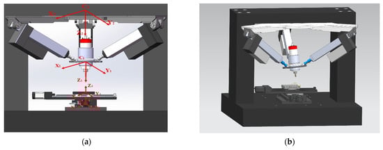
Figure 16.
XY-3-RPS hybrid robot model simulation: (a) 3D modeling diagram of XY-3-RPS hybrid robot; (b) motion simulation diagram.
7. Discussion
The trajectory planning method proposed in this paper, based on automatic partitioning with enhanced curvature characteristics, effectively improves the accuracy and continuity of trajectories in free-form surface polishing. By dynamically adjusting the step size, the method enables fine processing of high-curvature regions and efficient processing of low-curvature regions. The hybrid optimization framework, combining genetic algorithm (GA) and local search (LS), further optimizes both the overall distribution and local smoothness of the trajectory. The simulation and interference checking results confirm the feasibility and stability of the method on the XY-3-RPS hybrid robot platform, which demonstrates excellent processing performance and potential for engineering applications.
Future research could focus on further optimizing the dynamic partitioning algorithm to enhance its adaptability to complex curvature changes. Additionally, intelligent optimization methods, such as reinforcement learning and multi-objective evolution, could be introduced to improve the intelligence and global performance of trajectory planning. The machining effect of the trajectory should be verified through actual machining experiments to improve the method’s practicality. Furthermore, the method can be extended to other free-form surfaces and multi-axis robot platforms, promoting its broader application in complex manufacturing scenarios. The method can be extended to other types of free-form surfaces and multi-axis robot platforms, further promoting its wide application in complex manufacturing scenarios.
The method proposed in this paper is based on point cloud preprocessing and B-spline surface fitting, demonstrating good stability and applicability for workpiece surfaces of conventional complexity with strong potential for engineering applications. However, for complex surfaces with high curvature, intricate details, or multiple topologies, the fitting accuracy and stability of the method may decrease. Complex surface features may cause the accumulation of fitting errors, which affect the continuity and smoothness of trajectory planning, thereby limiting the final processing outcome. Therefore, it is recommended that the performance and application limits of the method on complex surfaces be further evaluated in future work to ensure its robustness and reliability across a wider range of application scenarios. Additionally, the hardware devices currently used are highly accurate and powerful, but the method’s performance on low-configuration hardware platforms has yet to be tested. Future research will focus on enhancing the algorithm’s robustness, reducing its dependence on hardware, and verifying its applicability in various processing environments.
8. Conclusions
This paper proposes a trajectory planning method to address the issues of poor accuracy, weak continuity, and difficulty in processing high-curvature areas in freeform surface polishing. The method is based on automatic partitioning with improved curvature characteristics and incorporates a hybrid optimization framework combining genetic algorithm (GA) and local search (LS) for global optimization and local fine-tuning of the trajectory. By dynamically partitioning high- and low-curvature regions and smoothing the boundaries, the adaptability and continuity of the trajectory are enhanced. This approach overcomes the issues of oversimplification and trajectory mutation associated with traditional fixed-threshold partitioning. The hybrid optimization results of GA and LS demonstrate significant improvements in trajectory length, maximum curvature, number of angle overruns, and other key metrics, leading to notable gains in machining accuracy and efficiency. Simulation analysis confirms the feasibility and stability of the method in the XY-3-RPS hybrid robot system, highlighting its strong potential for engineering applications. Future work will focus on further enhancing the adaptability of the partitioning algorithm and expanding its applicability in complex processing scenarios by integrating a multi-objective optimization strategy.
Author Contributions
Conceptualization, J.A. and X.S.; data curation, J.A. and X.M.; formal analysis, J.A. and X.M.; funding acquisition, X.S.; investigation, J.A. and X.M.; methodology, J.A. and X.S.; resources, J.A. and X.S.; software, J.A.; supervision, X.S.; validation, J.A. and X.S.; visualization, X.S.; writing—original draft, J.A.; writing—review and editing, X.S. All authors were updated at each stage of manuscript processing, including submission, revision, and revision reminder via emails from our system or the assigned Assistant Editor. All authors have read and agreed to the published version of the manuscript.
Funding
This research was funded by the National Natural Science Foundation of China (No. 52365056).
Data Availability Statement
The data presented in this study are available upon request from the corresponding author.
Acknowledgments
We thank all the authors for their contributions and efforts and the anonymous reviewers for their valuable comments.
Conflicts of Interest
The authors declare no conflicts of interest.
References
- Werner, A.; Poniatowska, M. Planning the Coordinate Measurements of a Freeform Surface after Milling based on a CAD Model Simulating the Surface after Machining. Acta Mech. Autom. 2024, 18, 730–736. [Google Scholar] [CrossRef]
- Deng, X.; Hu, P.; Li, Z.; Zhang, W.; He, D.; Chen, Y. Reinforcement Learning-based five-axis continuous inspection method for complex freeform surface. Robot. Comput.-Integr. Manuf. 2025, 94, 102990. [Google Scholar] [CrossRef]
- Jiang, C.; Zhang, E.; Zhang, W.; Hu, J.; Guo, J.; Li, X. Simulation and experimental verification of the precision finishing method for optical free-form surface segmentation. PLoS ONE 2025, 20, e0314489. [Google Scholar] [CrossRef] [PubMed]
- Song, X.; Wang, X.; Wang, J.; Fu, H. Design and Analysis of an Inverted XY-3RPS Hybrid Mechanism for Polishing of Complex Surface. Recent Pat. Mech. Eng. 2022, 15, 422–437. [Google Scholar] [CrossRef]
- Wang, J.; Wang, S.; Wen, Y.; Song, X. Design and kinematic simulation of the XY-3-RPS hybrid robot. Light Ind. Mach. 2020, 38, 5–10. [Google Scholar]
- Dimitrov, D.; Karachorova, V.; Szecsi, T. System for controlling the accuracy and reliability of machining operations on machining centres. Procedia Eng. 2013, 63, 108–114. [Google Scholar] [CrossRef]
- Li, W.; Fan, B.; Shi, C.; Wang, J.; Zhuo, B. A path planning method used in fluid jet polishing eliminating lightweight mirror imprinting effect. In Proceedings of the 7th International Symposium on Advanced Optical Manufacturing and Testing Technologies (AOMATT 2014), Harbin, China, 26–29 April 2014; Volume 9281. 92811H-92811H-8. [Google Scholar] [CrossRef]
- Dong, Z.; Zhang, X.; Yang, W.; Lei, M.; Zhang, C.; Wan, J. Ant colony optimization-based method for energy-efficient cutting trajectory planning in axial robotic roadheader. Appl. Soft Comput. 2024, 163, 111965. [Google Scholar] [CrossRef]
- Myasoedova, M.T.; Panchuk, L.K. Geometric model of generation of family of contour-parallel trajectories (equidistant family) of a machine tool. J. Phys. Conf. Ser. 2019, 1210, 012104. [Google Scholar] [CrossRef]
- Chen, M.; Zhu, Z.; Zhu, Y.; Han, T. A New Method for spherical tool polishing Trajectory Planning considering material removal Characteristics. Comput. Integr. Manuf. Syst. 2023, 29, 864–873. [Google Scholar] [CrossRef]
- Zheng, Y.X. Multi-Directional Trajectory Planning for Surface Polishing. Master’s Thesis, South China University of Technology, Guangzhou, China, 2018. [Google Scholar]
- Amersdorfer, M.; Kappey, J.; Meurer, T. Real-time freeform surface and path tracking for force controlled robotic tooling applications. Robot. Comput.-Integr. Manuf. 2020, 65, 101955. [Google Scholar] [CrossRef]
- Wang, Z.; Li, Y.; Shuai, K.; Zhu, W.; Chen, B.; Chen, K. Multi-objective trajectory planning method based on the improved elitist non-dominated sorting genetic algorithm. Chin. J. Mech. Eng. 2022, 35, 7. [Google Scholar] [CrossRef]
- Baghli, Z.F.; Bakkali, E.L.; Lakhal, Y. Optimization of arm manipulator trajectory planning in the presence of obstacles by ant colony algorithm. Procedia Eng. 2017, 181, 560–567. [Google Scholar] [CrossRef]
- Zhu, A.; Wang, Z. Trajectory planning of rotor welding manipulator based on an improved particle swarm optimization algorithm. Adv. Comput. Signals Syst. 2024, 8, 122–129. [Google Scholar] [CrossRef]
- Gui, H. Research on trajectory optimization of robot polishing freeform surfaces. Sci. Technol. Consult. Her. 2007, 11, 3–4. [Google Scholar] [CrossRef]
- Liu, Q. Research on Polishing Trajectory and Material Removal Optimization Based on CCOS. Master’s Thesis, Jilin University, Changchun, China, 2022. [Google Scholar]
- Kazim, M.; Hong, J.; Kim, G.M.; Kim, K.-K.K. Recent advances in path integral control for trajectory optimization: An overview in theoretical and algorithmic perspectives. Annu. Rev. Control 2024, 57, 100931. [Google Scholar] [CrossRef]
- Grubler, A.; Kutzbach, H. The synthesis of planar mechanisms. J. Appl. Mech. 1963, 30, 10–17. [Google Scholar]
- Luo, S.; Sun, Y.; Zhai, J.; Zhang, Q.; Chang, X. Optimization of free form surface in bulge formed joint based on isogeometric analysis. Iran. J. Sci. Technol. Trans. Mech. Eng. 2024, 49, 1069–1083. [Google Scholar] [CrossRef]
- Zhao, P.; Gao, F.; Guo, K.; Zhang, E.; Li, S. Trajectory optimization of B-splines interpolation based on dynamic error adjustment. J. Phys. Conf. Ser. 2024, 2760, 012038. [Google Scholar] [CrossRef]
- Zhaohui, G.; Arman, S.; Bopaya, B. A framework of tolerance specification for freeform point clouds and capability analysis for reverse engineering processes. Int. J. Prod. Res. 2022, 60, 7475–7491. [Google Scholar] [CrossRef]
- Lin, Y.; Yang, H.; Weihong, W.; Yehua, S.; Xin, J. Processing of multitemporal 3D point cloud data for use in reconstructing historical geographic scenarios. Sens. Mater. 2022, 34, 4551. [Google Scholar] [CrossRef]
- Harmening, C.; Butzer, R. Improving the approximation quality of tensor product B-spline surfaces by local parameterization. J. Appl. Geod. 2024, 18, 575–596. [Google Scholar] [CrossRef]
- Hao, J.; He, D.; Li, Z.; Hu, P.; Chen, Y.; Tang, K. Efficient cutting path planning for a non-spherical tool based on an iso-scallop height distance field. Chin. J. Aeronaut. 2024, 37, 496–510. [Google Scholar] [CrossRef]
- Cervone, A.; Manservisi, S.; Scardovelli, R.; Sirotti, L. Computing interface curvature from height functions using machine learning with a symmetry-preserving approach for two-phase simulations. Energies 2024, 17, 3674. [Google Scholar] [CrossRef]
- Gao, X.; Li, R.; Wang, B.; Li, W.; Zhao, Z. Automatic partitioning algorithm for profile feature processing of aircraft structural components. J. Aeronaut. 2021, 42, 32–42. [Google Scholar]
- Duan, P. Research on Robot Trajectory Optimization for Polishing Small-Curvature Freeform Surfaces. Master’s Thesis, Anhui University of Engineering, Wuhu, China, 2023. [Google Scholar]
- Jia, R.; Li, H.; Wei, F.; Xu, Y.; Zhou, Y. Polar weld seam recognition and robot trajectory generation technology based on 3D point cloud. Trans. China Weld. Inst. 2024, 45, 50–54. [Google Scholar]
- Yang, H.L. Adaptive robotic trajectory generation and control strategy for complex curved surface welding. Off. Autom. 2024, 29, 62–64. [Google Scholar]
- Duan, H.Y.X.; Zhang, Y.; Chen, H.R.; Zhang, Q.Y. Review on trajectory planning and optimization of industrial robots. Agric. Equip. Veh. Eng. 2023, 61, 54–57. [Google Scholar]
Disclaimer/Publisher’s Note: The statements, opinions and data contained in all publications are solely those of the individual author(s) and contributor(s) and not of MDPI and/or the editor(s). MDPI and/or the editor(s) disclaim responsibility for any injury to people or property resulting from any ideas, methods, instructions or products referred to in the content. |
© 2025 by the authors. Licensee MDPI, Basel, Switzerland. This article is an open access article distributed under the terms and conditions of the Creative Commons Attribution (CC BY) license (https://creativecommons.org/licenses/by/4.0/).