Article

Pressure Control in the Pump-Controlled Hydraulic Die Cushion Pressure-Building Phase Using Enhanced Model Predictive Control with Extended State Observer-Genetic Algorithm Optimization

1
School of Mechanical Engineering, Yanshan University, Qinhuangdao 066004, China
2
School of Mechanical Engineering, Hebei University of Architecture, Zhangjiakou 075000, China
3
Mechanical and Electrical Engineering, Xinjiang Institute of Engineering, Urumqi 830023, China
*
Authors to whom correspondence should be addressed.
Actuators 2025, 14(6), 261; https://doi.org/10.3390/act14060261
Submission received: 13 April 2025 / Revised: 19 May 2025 / Accepted: 21 May 2025 / Published: 25 May 2025
(This article belongs to the Section Control Systems)

Abstract

With the enhancement of safety performance requirements in the car manufacturing field, the quality standards for the sheet molding process have imposed higher demands. However, during the pressure-building phase of pump-controlled hydraulic die cushion systems, the combined effects of high-order dynamics, system uncertainties, and strong nonlinearities pose significant challenges to maintaining precise control and dynamic response performance of the blank holder force (BHF). To address these challenges, we propose an intelligent model predictive control (MPC) strategy that synergistically integrates an extended state observer (ESO) for disturbance compensation with parameters optimized by a genetic algorithm (GA). The mathematical model and state-space model of the system are established. Subsequently, the ESO is integrated with MPC to enable active compensation for internal and external disturbances. The GA is employed to optimize the controller parameters within the MPC framework. Finally, a simulation testbed for the pump-controlled hydraulic die cushion experimentally validates the process. Experimental results demonstrate that compared to MPC and conventional PID control, the proposed strategy achieves significant reductions in pressure overshoot (0.87% and 1.8% at 100 bar; 3.3% and 5.9% at 200 bar), pressure-building time (13.9% and 31.4% at 100 bar; 6.7% and 11.5% at 200 bar), and stroke length (10.5% and 32% at 100 bar; 11.5% and 28.1% at 200 bar). This validates its effectiveness in enhancing both control precision and dynamic response performance, providing a reliable solution for large-scale applications of pump-controlled hydraulic die cushions in high-dynamic stamping scenarios.

1. Introduction

Hydraulic die cushions, as critical components in mechanical presses, are widely used in the stamping and molding process of automotive coverings [1,2]. Traditional hydraulic die cushions mostly employ a throttling speed control system regulated by an electrohydraulic servo valve. This approach has the disadvantages of low energy efficiency, large heat generation, and cumbersome troubleshooting [3,4]. The pump control system adopts volume control, which technically avoids the throttling loss and can realize efficient operation [5,6,7,8].
However, the pump control system exhibits several defects, including higher-order dynamic characteristics, system uncertainty, and strong nonlinearity. These issues present challenges in maintaining precise control of the BHF and ensuring optimal dynamic response performance [9,10,11]. The accuracy of the hydraulic die cushion blanking force directly affects the forming quality of automotive cover parts. In this process, the BHF between the sheet and the mold directly affects the magnitude of the friction force [12,13]. Too much BHF will hinder the flow of sheet metal, resulting in sheet tearing, and insufficient BHF results in sheet wrinkles [14,15]. Therefore, the study of the pump-controlled hydraulic cushion pressure control strategy with high dynamic accuracy has significant research value for enhancing molding quality. The hydraulic die cushion’s design is depicted diagrammatically in Figure 1.
There are relatively few studies on hydraulic die cushion BHF control, and most of the pressure control studies have focused on valve-controlled systems. Aiming at the problem of insufficient pressure control accuracy caused by the nonlinearity and indeterminacy of the valve-controlled system, Sun et al. [16] presented a feedback-linearization-based integral sliding mode controller, with its asymptotic stability rigorously proven via Lyapunov’s direct method, and remarkably improved the system force tracking accuracy. Trojaola et al. [17] proposed an iterative learning control algorithm based on fourth-order low-pass filtering, which optimizes the zero-phase filtering by suppressing the dynamic interference of the valves, significantly shortens the build-up time of the pressure signal of the hydraulic cylinders, and reduces the amount of overshooting. Sun [18] presented a real-time control force algorithm without force/pressure feedback, which calculates the joint torque in real computation, thus realizing precise control of the output force. Li et al. [19] presented an adaptive control approach to significantly suppress the uncertainty in pressure dynamics through online identification of hydraulic stiffness and valve flow characteristic parameters. Ji et al. [20] proposed a disturbance rejection adaptive control approach for force control of a main cylinder, which significantly enhances the ability of precise pressure control. Kim [21] presented a learning force controller for hydraulic actuators, adopting deep neural networks to construct an inverse model to achieve high-precision force trajectory tracking, which significantly improves the tracking performance. Shang [22] presented a pressure control arithmetic based on an array of switching valves, which realizes dynamic pressure prediction and control by modeling the time-pressure characteristics of the valves and designing the observer of the unknown input states, optimizing the system pressure control accuracy. Helian et al. [23] designed an adaptive robust back-stepping control strategy to deal with the dynamic nonlinearities and parameter uncertainties in the variable displacement axial piston pump system for achieving accurate pressure tracking.
With the superimposed effect of increased sustainable development requirements and rigid cost-effectiveness constraints, there is an increasing need to further reduce energy consumption while achieving high-precision motion control [24,25,26]. Some scholars have begun conducting studies to enhance pressure control in pump-controlled systems. Hao et al. [27] used the ESO to realize the online estimation of disturbance force and dynamically compensated actuator disturbance force through the hydraulic cylinder so that the system works in the preset load interval. Pfizenmaier et al. [28] designed a new type of test bench for dynamic pressure load simulation, which adopts the hydraulic half-bridge structure in the pump on both sides of the independent control side to realize the pressure closed loop, and designed an error-based adaptive controller to improve the control accuracy. Zhao et al. [29] proposed an electrohydraulic cylinder system with a one-motor–one-pump configuration utilizing centralized pressure control, which enables passive load retention via active pressure adjustment in hydraulic circuits, and its pressure control logic covers the dynamic pressure compensation and the closed-loop regulation of the steady-state pressure under four-quadrant operating conditions. Cao et al. [30] presented a controlled state reconstruction-based adaptive robust pressure control technique with noise suppression for electrohydraulic braking systems, and the algorithm achieves precise and accurate pressure regulation. Some scholars have also studied the pressure control of the pump-valve system by combining the virtues of pump-controlled and valve-controlled systems. Ba et al. [31] designed a new pump–valve composite drive system and proposed a new force control strategy based on quantitative feedback theory and a disturbed torque observer, which improves the force control property. Yu et al. [32] designed a pressure control approach combining follow error compensation and loading compensation control to enhance the system pressure control accuracy. Tan et al. [33] designed a direct-drive pump–valve coordinated line control dynamical unit to meet the demand for precise braking force control for autonomous driving and proposed an improved adaptive integral robust control method based on a novel adaptive law and perturbation compensation. Cheng et al. [34] improved the dynamic performance of a multi-actuator system by proposing a decoupling compensator based on combined pump–valve control that reduces velocity and pressure oscillations. There are also a number of methods that have been widely used to solve the control problem. Yang et al. [35] created a new state-filtered disturbance suppression control architecture based on powerful command filtering anti-stepping measures that can eliminate the detrimental effects of “complexity explosion” and improve control accuracy. Yang et al. [36] proposed a novel disturbance–compensation-based multilayer neural network adaptive controller for high-order uncertain nonlinear systems.
In general, the valve-controlled, pump-controlled, and pump–valve composite methods for hydraulic die cushion pressure control have established an important theoretical foundation. However, the existing studies still face challenges in meeting the requirements for high-dynamic pressure fluctuation suppression and nonlinear disturbance compensation under practical high-inertia and heavy-load operating conditions of pump-controlled hydraulic die cushions [37,38,39]. In the above studies on pressure control challenges, conventional MPC demonstrates capability in handling pressure constraints [13]. However, its weight matrix requires empirical parameter tuning and exhibits sensitivity to nonlinear disturbances like flow pulsations and friction, resulting in a limited dynamic response. Although the ESO can estimate perturbations [24], is difficult to match the multi-step prediction demand through only single-step feed-forward compensation because it is not deeply integrated with the rolling optimization of MPC. The GA is mostly used for energy efficiency optimization and parameter tuning in pump control systems [26], and the existing approach fails to incorporate the pressure tracking accuracy and the dynamic characteristics of the pressure-building phase into a unified optimization framework. In addition, methods based on online parameter identification recognize the suppression of uncertainty [19], making it difficult to meet the real-time control requirements because of model dependency with high computational complexity.
Therefore, this paper proposes the ESO-GA-MPC composite control strategy to realize the deep integration of nonlinear disturbance suppression, parameter optimization, and rolling prediction. By directly inputting the total perturbations, such as friction, flow pulsations, etc., estimated by the ESO, as well as the velocity observation signal into MPC, a dynamic compensation mechanism in the framework of multi-step rolling optimization is formed, which significantly improves the anti-disturbance capability. Concurrently, the GA is used to adjust the weight matrices Q and S of MPC to optimize the performance index of the MPC controller, and the parameter optimization enables MPC to reach the global optimization under complex working conditions. The method combines the ability of the ESO to correct local perturbations in real time with the global parameter optimization of the GA, circumvents the dependence on accurate models of traditional methods, reduces the computational complexity, and provides an innovative solution for overshooting suppression and pressure build-up acceleration in highly dynamic hydraulic systems.
The remainder of this paper is organized as follows. Section 2 establishes mathematical models and state-space representations for key system components. Section 3 proposes a control scheme for the pressure-building process in the pump-controlled hydraulic die cushion. Section 4 describes the pump-controlled hydraulic die cushion simulation test bed and experimentally verifies the effectiveness of the proposed pressure control method. Finally, Section 5 concludes the research findings.

2. System Modeling

2.1. Mathematical Modeling of Swashplate Axial Piston Pumps

Swashplate axial piston pumps are particularly suitable for pump-controlled hydraulic die cushions by virtue of their compact structure and high working pressure. This study employs a nine-piston axial piston pump, chosen for its low flow pulsation characteristics. The pump configuration effectively reduces fluctuations in hydraulic system flow and ensures stability during the pressure-building phase. Through an in-depth analysis of the pump’s pulsation mechanism and a comprehensive consideration of the coupling effects of leakage and other nonlinear factors, we constructed a nonlinear dynamic mathematical model of the pump.
Incorporating fluid leakage effects, the flow rate equation for the axial piston pump is established.
Q a = ω d 2 4 N R tan β C t p p L + d m φ 1 , ω , t
where d is the plunger diameter, R is the radius of the trajectory of the plunger axis in the cylinder, β is the inclination angle of the swash plate in the plunger pump, φ 1 is the rotation angle of the first plunger, ω is the rotational speed of the plunger pump, N is the total number of plungers inside the plunger pump, C t p is the total leakage coefficient of the plunger pump, p L is the pressure difference across the plunger pump, and d m is the time-varying disturbance of the remaining pulsating portion of the flow.
The mathematical model of the quantitative piston pump with an odd plunger configuration in this paper can be expressed as:
Q L = N p D p C t p p L + d m φ 1 , ω , t
where D p is the displacement of the piston pump and N p is the quantitative piston pump speed.

2.2. Mathematical Model of the Servo Motor

In pressure control systems, the servo motor functions as the primary actuator to implement control algorithms. To simplify the mathematical modeling for the servo motor, it is common practice to neglect the effects of core saturation, iron losses, rotor damping, and other factors on servo motion.
The stator magnetic chain equation of the servomotor in the d q coordinate system is defined as:
ψ d = L d i d + ψ f ψ q = L q i q
where L d and L q represent the equivalent inductances of the stator along the d q axial, i q and i d are the d q axial current measure of the stator, and ψ f corresponds to the permanent magnet flux.
Substituting Equation (3) into the stator voltage equation in coordinates, the following can be obtained:
U d = R s i d + L d d d t i d ω e L q i q U q = R s i q + L q d d t i q + ω e L d i d + ψ f
where R s is the stator winding resistance and ω e is the rotor angular velocity.
The electromagnetic torque equation is:
T e = 3 2 p n ψ f i q + L d L q i d i q
where T e is the internal electromagnetic torque and p n is the pole logarithm.
The equation of motion for the motor is:
T e T L = J L d ω m d t + D ω m
where T L is the load torque, J L is the moment of inertia of all the rotating axes converted to the rotating axes, ω m is the motor mechanical angular velocity, and D is the motor damping coefficient.
The vector control method of i d = 0 is to decouple the vectors in the motor on the d q axis. When the i d = 0 vector control method is used, no magnetic recession occurs, yielding a simplified torque equation:
T e = 3 2 p n ψ f i q
In Equation (7), p n and ψ f are fixed parameters of the motor. Consequently, the electromagnetic torque of the motor can be regulated by controlling i q .
By defining K t = 1.5 p n ψ f , Equation (7) is simplified to:
T e = K t i q
where K t is the torque sensitivity factor.
Under rated operating conditions, the induced electromotive force inside the armature winding is:
E = K e ω e
where K e is the speed constant.
According to Equations (8) and (9), the loop voltage equation can be derived as:
U q = L q d i q d t + R s i q + K e ω e

2.3. Mathematical Modeling of the Hydraulic Cylinder

The hydraulic cylinder functions as the actuator in the pump-controlled hydraulic die cushion system, with its structural configuration illustrated in Figure 2.
In accordance with the structure diagram of the hydraulic cylinder, the force balance equation is:
A p p L = m t d 2 x p d t 2 + B p d x p d t + K x p + F L + F f
where m t is the total mass of the piston and load converted to the piston, B p is the viscous damping coefficient, K is the equivalent stiffness of the mechanical load and the plate, x p is the piston displacement, F L is the external load force, F f is the nonlinear friction on the piston, A p is the piston effective area, and p L is the cylinder differential pressure.
The continuity equation for the symmetric hydraulic cylinder flow q L is:
q L = A p d x p d t + C t c p L + V t 4 β e d p L d t C t c = C i c + C e c
where C t c is the total leakage coefficient of the hydraulic cylinder system, β e is the effective bulk elastic modulus, V t is the general compressed capacity, C i c is the inside leakage factor of the cylinder, and C e c is the external leakage coefficient of the cylinder.
According to Stribeck’s friction theory, the mathematical model of the variation in friction with velocity can be obtained as:
F f = F f d ( v )                       ( v 0 ) F e s i g n ( F e )         ( v = 0 , F e < F j )   F f s i g n ( F e )         ( v = 0 , F e F j )
where F f is the frictional force, v is the relative velocity of the friction pair, F j is the maximum static frictional force, F f d is the dynamic friction, and F e is the external force.
The dynamic friction F f d equation is:
F f d = s i g n ( v ) F k + ( F j F k ) exp v v s τ + B v
where F k is the coulomb frictional force, v s is the Stribeck velocity, B is the viscous friction coefficient, and τ is an empirical parameter, typically ranging between 0.5 and 2.

2.4. State-Space Model

The following table lists the key parameters required to construct the state-space equations for the pump-controlled hydraulic mold cushioning system in Section 2.4, as shown in Table 1.
The state-space equations of the system are established by combining Equations (2), (11) and (12). Defining the system control variable as N p , the state variables, control variables, and output variables of the pump-controlled hydraulic die cushion system are:
x = x 1 x 2 x 3 T = x p x ˙ p p L T u = N p T y = x p 0 p L T
The state-space equation for the nonlinear model is:
x ˙ 1 = x 2 x ˙ 2 = K m t x 1 B p m t x 2 + A p m t x 3 + F L m t + F f m t x ˙ 3 = 4 β e A p V t x 1 4 β e C t V t x 3 + 4 β e D p V t u + 4 β e V t d m φ , ω , t y = C x
The system is affected by nonlinear friction, piston pump pressure pulsations, and other factors that cannot be directly used in the MPC algorithm based on the linear superposition principle. The derivation process first requires linearizing the pump-controlled hydraulic die cushion system.
Equation (16) is the standard state-space equation. By considering the nonlinear friction and plunger pump pulsation as time-varying disturbances, the system is rewritten as:
x ˙ = f x , u = A x + B u + D y = C x
where A is a 3 × 3 matrix, B is a 3 × 1 matrix, C is a 3 × 3 matrix, and D is a 3 × 1 matrix. Their specific values are given in Equation (18).
A = 0 1 0 K m t B p m t A p m t 0 4 β e A p V t 4 β e C t V t B = 0 0 4 β e D m V t C = 1 0 0 0 0 0 0 0 1
This paper establishes a pump-controlled hydraulic die cushion system model based on the state-space equation, linearizes the nonlinear system by using the Jacobi matrix linearization method, and then converts the continuous domain model into a discrete form suitable for the digital controller by the discretization method. The derivation process follows the system modeling process of “linearization first, discretization second”.
Consider the following nonlinear hydraulic die cushion system:
x t + 1 = f x t , u t = A x t + B u t + D y t = C x t
The simplification of Equation (19) can be obtained by carrying out a Taylor-level expansion at any one of the stabilization points x ^ 0 , u ^ 0 , neglecting the higher-order terms, and retaining the first order:
x t + 1 = f x ^ 0 , u ^ 0 + f x x ^ 0 , u ^ 0 x t x ^ 0 + f u x ^ 0 , u ^ 0 u t u ^ 0
The simplified form can be expressed as:
x t + 1 = f x ^ 0 , u ^ 0 + J f x t x t x ^ 0 + J f u t u t u ^ 0
In the control time domain, x ^ 0 and u ^ 0 are invariant quantities applied to the pump-controlled hydraulic die cushion, and the following settings are made for the system:
A t , 0 = J f x , B t , 0 = J f u δ x t = x t x ^ 0 δ u t = u t u ^ 0 δ x t + 1 = x t + 1 x ^ 0 t + 1
Then, the system can be expressed as:
δ x t + 1 = A t , 0 δ x t + B t , 0 δ u t
Equation (23) is a linear time-variant system that explains the relationship between nonlinear state variables and reference quantities during linearization. This model can be reformulated as follows:
        x ˙ t = A t , 0 x t + B t , 0 x t + d t , 0 t d t , 0 t = x ˙ 0 t A t , 0 x ^ 0 t B t , 0 u ^ 0 t
The discrete state-space equation is:
x k + 1 = A k , t x k + B k , t u k + d k , t
The state matrix, control matrix, and disturbance matrix of each state in the discrete system are:
A k = I + T A t B k = T B t d k = x ^ k + 1 A k x k B k u k

3. Control Scheme

3.1. Algorithmic Architecture
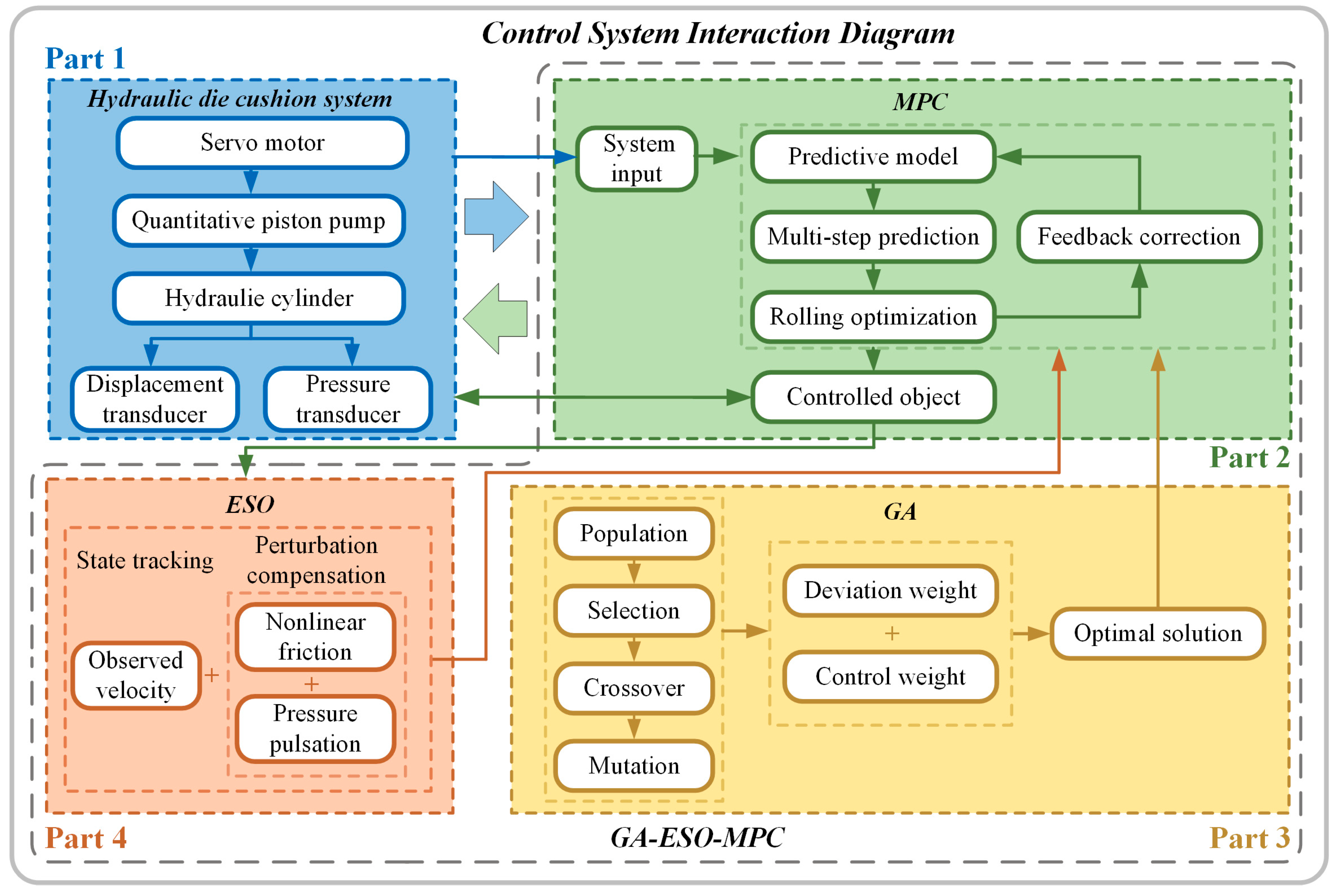
The controller must be designed with a multi-faceted approach to address nonlinear disturbances in the pump-controlled hydraulic die cushion system and improve its rapid response performance. Figure 3 and Figure 4 show the real-time interaction diagram and overall control strategy.
(1)
The MPC algorithm is adopted to address upper and lower limit constraints essential for the effective pressure control of the hydraulic die cushion during the pressure-building process. This control strategy designs the corresponding output prediction equation based on the system model, expresses the constraints as a quadratic programming problem, and dynamically updates control policies in response to environmental disturbances, demonstrating enhanced robustness.
(2)
The ESO was designed to tackle internal disturbances and challenges in observing the velocity signal. This observer estimates and compensates for nonlinear friction and piston pump pulsation and observes the velocity information of the hydraulic cylinders required by the MPC algorithm.
(3)
The GA is used for parameter optimization within the complex context of MPC, which necessitates the configuration of numerous parameters. The GA optimizes the output volume deviation weight matrix Q and the system control volume weight matrix S through iterative processes, ensuring that MPC achieves optimal control effect.

3.2. Control Program Design

3.2.1. Incremental Prediction Model Design

The output of the pump-controlled hydraulic die cushion is added to the discretized model to obtain an overall linear time-varying system.
x k + 1 = A k , t x k + B k , t u k + d k , t y k = C k , t x k
To reduce the controller’s computational load, the predictive model uses an incremental state-space as a basis for rolling optimization.
A new variable is designed for the system:
ξ k = x k t u k 1 t
The revised state-space equations of the system are formulated in incremental form as:
ξ k + 1 t = A k , t B k , t 0 m × n I m ξ k t + B k , t I m Δ u k t + d k , t 0 m y k t = C k , t 0 m ξ k t
The system output at moment k can be obtained by iterating over the forecasted steps y k t , i.e., the step k system output is predicted at moment t as:
y k t = C ˜ k , t i = t k 1 A ˜ k , t ξ t t + i = t k 1 C ˜ k , t j = i + t k 1 A ˜ j , t B ˜ j , t Δ u i t + d ˜ i t
When the prediction step is set to exceed the control step, the increment of the control variable is the same value, and the system output sequence over the forecast horizon H p as:
Y t = Λ t ξ t t + Θ t Δ U t + Γ t Φ t
where Y t is the output prediction vector for the future H p step, Λ t is the influence matrix from the initial state ξ t t to the output prediction Y t , Θ t is the influence matrix of the control inputs, Γ t is the influence matrix of the disturbance term, and Φ t is the disturbance estimation vector for the future H p step.
The output quantities of the system are defined as follows:
y t t = y t r t t y c t t y s c t t T
where y t r R p y , y c R p c , and y s c R p u . y t r , y c , and y s c are the controlled output, the soft restriction output, and the soft restraint output, respectively.
The predicted tracking output Y t r t over the prediction horizon H p is formally defined as:
Y t r t = η t r t + 1 t η t r t + 2 t η t r t + H p t T Y t r t = Ψ t r Y t
where Ψ t r R , and the newly added control output parameter of the system can be expressed as:
Ψ t r = I p y × p y 0 p y × p c 0 p y × p u 0 p y × p y 0 p y × p c 0 p y × p u 0 p y × p y 0 p y × p c 0 p y × p u 0 p y × p y 0 p y × p c 0 p y × p u 0 p y × p y 0 p y × p c 0 p y × p u I p y × p y 0 p y × p c 0 p y × p u
By synthesizing Equations (31) and (33), the predicted value of the predicted tracking output Y t r t over the prediction horizon H p is calculated as:
Y t r t = Λ t r t ξ t t + Θ t r t Δ U t + Γ t r t Φ t
where Λ t r t = ψ t r Λ t , Θ t r t = Ψ t r Θ t , and Γ t r t = ψ t r Γ t .
The hard-constrained output Y c t and soft-constrained output Y s c t in the prediction horizon H p can be computed in the form of a similar equation.
The predicted values in the prediction time domain are derived from the system state quantities ξ k | t at time t , the system control quantities u k 1 | t at the previous time, and the system control increments Y t r t computed by solving in the control horizon H c .

3.2.2. Objective Function Design

When solving for the optimal control output within each prediction step, the model does not necessarily have an optimal feasible solution. By introducing slack variables to adjust the objective function, the solved control quantity has optimal control.
J ξ t , u t 1 , Δ u , ε = i = 1 H p Y t r t + i t Y r e f t + i t Q 2 + i = 0 H c 1 Δ u t r t + i t R 2 + i = 0 H c 1 u t r t + i t S 2 + ρ ε 2
where ρ is the weight factor and ε is the slack factor.
The first term in Equation (36) expects the error between actual and predicted output values to express the pressure control accuracy. The absolute value of the control increment in the second term indicates the constraint size of the system on the control amount, ensuring that the system does not fluctuate greatly. The third term expresses the penalization strategy of the system, which enhances control accuracy while minimizing input.

3.2.3. Working Condition Constraints

The pump-controlled hydraulic die cushion system needs to impose constraints on both the control variables and their increments to ensure smooth pressure buildup and prevent significant abrupt changes in rotational speed. The constraint ranges for each system variable are detailed in Table 2.
The error of the output quantity within H p can be formulated as:
E t = Λ t r t ξ t t + Θ t r t Δ U t + Γ t r t Φ t Y r e f t
The system’s future moment output expression is brought into Equation (32), and by calculating a series of corresponding matrices, the objective form of its optimization is treated as:
J ξ t , u t 1 , Δ u , ε = 1 2 Δ U t ε Θ t T Q Θ t T + R 0 0 ρ Δ U t ε T + 2 E t T Q Θ t 0 Δ U t ε T + E t T Q E t
The basic principle of the quadratic programming problem is to find an n -dimensional vector x , such that under the restriction A 1 x 1 b 1 , f x 1 is minimized, and f x 1 is:
f x 1 = 1 / 2 x 1 T Q 1 x 1 + c T x 1
where A is an m × n -dimensional matrix; b is an m -dimensional vector; c is an n -dimensional vector; Q is an m × n -dimensional symmetric matrix; and x 1 T Q x 1 is a quadratic matrix.
By solving the final solution within each control cycle of the standard form of the quadratic programming problem, a series of optimal control increments within H c will then be obtained, as defined below:
Δ U t * = Δ u t * Δ u t + 1 * Δ u t + N c 1 * T
Acting on the first term in Equation (40) on the system, the final control quantities can be introduced:
u t = u t 1 + Δ u t *
During the pump-controlled hydraulic die cushion build-up process, MPC generates an optimal control sequence by solving a quadratic programming problem in real time. After the algorithm applies the current control increment from Equation (41) to the system, it performs rolling prediction based on the latest state information and updates the control sequence through dynamic optimization. This iterative process fully utilizes the constraint processing capability of MPC to ensure that the pressure-building process simultaneously meets dynamic performance requirements and operational constraints in industrial control.

3.2.4. ESO Design

For the ESO, the state-space equation is rewritten according to Equations (16) and (35) as:
x ˙ p = x ˙ p x ¨ p = A p m t p L B p m t x ˙ p K m t x p p ˙ L = 4 β e D m V t ω + 4 β e V t K m p L + 4 β e A p V t x p + d
where d = 1 γ m t f t + 4 β e γ V t d m φ 1 , ω , t + d o ; f t denotes the external and time-varying friction of the system, d o denotes the modeling error and external disturbances and treats them as uncertain time-varying disturbances, and γ is the gain coefficient of the additional disturbances.
Because of the inherent uncertainties and nonlinearities of hydraulic systems, modeling errors and internal disturbances in d are important factors affecting the system performance. To ensure optimal controller operation during closed-loop pressure control, the time-varying disturbance term d in Equation (42) is expanded into a new state quantity x 4 , as formalized below:
x 4 = ω
For a fourth-order linear system, according to Equations (42) and (43), it is rewritten in the form of a dilated state observer, with reference to Prof. Han Kyung-ching’s core idea for the ESO [40]:
e = x 1 x ^ 1 x ^ ˙ 1 = x ^ 2 + β 1 e x ^ ˙ 2 = A p m t x ^ 3 B p m t x ^ 2 K m t x ^ 1 + β 2 e x ^ ˙ 3 = 4 β e D m V t u + 4 β e V t K m x ^ 3 + 4 β e A p V t x ^ 1 + β 3 e + x ^ 4 x ˙ ^ 4 = ω + β 4 e y = x 1
where x ^ 1 , x ^ 2 , and x ^ 3 are estimated system state variables, x ^ 4 represents the total disturbance estimation for the dynamical system, and β 1 , β 2 , β 3 , and β 4 are the gain coefficients of the ESO.
To accurately estimate and compensate for the system state variables x 1 , x 2 , x 3 , and x 4 in Equation (44), a method for determining the linear ESO gain is used, and the concept of bandwidth is employed to determine the gain parameters.
Dr. Zhiqiang Gao of Cleveland State University [41] proposed a deterministic linearly ESO gain side. The characteristic polynomial of the ESO is:
λ s = s 3 + β 1 s 2 + β 2 s + β 3
By choosing β i to make the system stable, the characteristic polynomial should satisfy the Hurwitz stability criterion. Therefore, the following characteristic equation can be taken to ensure that all roots of the system have negative real parts, where  ω > 0 .
λ s = s + ω 3
This is obtained by the binomial theorem.
β i = C 3 i ω i = 3 ! i ! 3 i ! ω i i = 1 , 2 , 3
where ω is the ESO bandwidth, the only parameter that the observer needs to be tuned to make parameter tuning easier.
The expression for the linear ESO of the pump-controlled hydraulic die cushion pressure control system can be obtained by Equations (44) and (47) as:
e = x 1 x ^ 1 x ^ ˙ 1 = x ^ 2 + 4 ω e x ^ ˙ 2 = A p m t x ^ 3 B p m t x ^ 2 K m t x ^ 1 + 6 ω 2 e x ^ ˙ 3 = 4 β e D m V t u + 4 β e V t K m x ^ 3 + 4 β e A p V t x ^ 1 + x ^ 4 + 4 ω 3 e x ˙ ^ 4 = ω + ω 4 e y = x 1
The designed ESO exhibits a bandwidth-dependent estimation performance. Increasing the observer bandwidth ω enhances disturbance and state estimation rates while simultaneously amplifying high-frequency measurement noise. Optimal bandwidth selection must therefore balance rapid system information acquisition with noise suppression to achieve accurate state observation and disturbance compensation.
According to Equation (31), the MPC algorithm must incorporate the hydraulic die cushion work into its control calculations when the system’s state variables—such as the hydraulic cylinder displacement, cylinder speed, system pressure, and control volume output signals—are the actual control of the hydraulic cylinder speed signal. It is difficult to collect the hydraulic cylinder displacement through the derivation of the system speed in this way, as it will be mixed with high-frequency noise, resulting in the obtained velocity signals being inaccurate. Through the ESO, the velocity signal is observed and introduced into the MPC algorithm to increase its stability.
According to Equation (48), it enables the ESO to estimate both internal and external disturbances, which are incorporated into the MPC algorithm to mitigate the effect of system perturbations on MPC.
According to the above equation, the model prediction is known in Equation (26):
d k = x ^ k + 1 A k x k B k u k
where x ^ k + 1 is obtained from the inputs and outputs of the nonlinear model of the system, and x ^ k + 1 is expanded and written out with state and control quantities. The discrete form state-space expression is:
x ^ ˙ 1 k + 1 = x 1 k + x 2 k d t x ^ ˙ 2 k + 1 = x 2 k K m t x 1 k d t B p m t x 2 k d t + A p m t x 3 k d t x ^ ˙ 3 k + 1 = x 3 k + 4 β e A p 3 V 0 x 1 k d t + 4 β e 3 V 0 K m x 3 k d t D ^ 4 β e D m 3 V 0 u k d t
where d t is the system discrete time quantity, D ^ is the system disturbance quantity estimated by the ESO, x 1 k is the system displacement feedback quantity, x 2 k is the velocity feedback quantity observed by the ESO, and x 3 k is the system pressure feedback quantity.

3.2.5. Parameter Optimization Based on the GA

The traditional MPC system has numerous parameters that can be time-consuming to adjust and do not guarantee stable system pressure for the hydraulic die cushion under complex working conditions. To improve the performance of the pump-controlled hydraulic die cushion during the pressure-building phase, the GA is employed to optimize the weight coefficients of the MPC algorithm, as illustrated in Table 3, for the parameters that require adjustment in the designed controller.
The selection of parameters H p , H c , R , S , ρ , and ω in Table 2 is mainly used for the importance of each input and output parameter of the system in the process of regulating the pressure building, as well as the determination of the coefficients of the bandwidth of external disturbances, which are simple to set and will not be studied further here. In this paper, the MPC algorithm is optimized for the output quantity deviation matrix Q and the control matrix S . The magnitudes of these two weight matrices significantly impact the real-time performance of the controller’s computation in solving the quadratic programming problem for the pressure-building phase. This, in turn, affects the effectiveness of the MPC algorithm. Therefore, optimizing these two weight matrices plays an important role.
Figure 5 shows the flow schematic diagram of the GA to optimize the controller parameters.
It is first normalized:
p e = 2 p r p p e , m i n p e , m a x p e , m i n 1 x e = 2 x p r x p x p e , m i n x p e , m a x x p e , m i n 1
The normalized parameters  p e , m a x and p e , m i n denote the maximum and minimum values of the pressure error between the actual pressure and the target pressure during pressure regulation; x p e , m a x and x p e , m i n denote the maximum and minimum values of the error between the actual stroke and the target stroke of the pressure regulation mechanism; p and x p denote the actual build pressure and pressure-building stroke; and p r and x p r denote the desired build pressure and pressure-building stroke.
The following comprehensive performance index is defined as:
e = σ p e + 1 σ x e
where σ is the weighted adjustment factor.
The method of integrating the absolute value of the error as a reference value has gained good application in engineering, so it is adopted as the adaptability function of the GA, i.e.,
J = 0 e d t
The optimization objective is determined as the output quantity deviation weight matrix Q of the model prediction controller and the weight matrix S of the system control quantity as:
K = Q S
To promote optimization efficiency, the weight matrix for the output deviation is set to Q 0 , 400 , and the weighting matrix for system control inputs is set to S 0 , 20 .
The parameters of the GA are set by combining Equations (51)–(54) with the actual working conditions of the hydraulic die cushion system. The crossover rate parameter is 0.5–0.97, and the mutation rate is 0.01–0.3. The system parameters are optimized to make the controller have the optimal control effect.
Figure 6 demonstrates a progressive enhancement in global optimization performance with increasing GA population size. When the number of populations is 50 or 60, although Figure 7 shows a faster pressure response, significant overshoot occurs. When the population size of the GA is 30, the best fitness value converges quickly, and the pressure overshoot is small, so the number of populations is chosen as 30. As shown in Figure 8, as the crossover rate increases, the best fitness value converges faster, and when the crossover rate takes a smaller value, the more the control pressure exceeds the given value in Figure 9, so the crossover rate is selected as 0.8. As shown in Figure 10, the MPC algorithm is not sensitive to the size of the variable probability value, and the pressure curve in Figure 11 does not change significantly. Mainly through the crossover operation, the GA inherits the information of the parent generation to search the interval, and the mutation operation adopts a method to enhance population diversity to carry out the inter-local search, so the mutation probability takes the value of 0.3.

4. Experimental Validation

4.1. System Setup

Figure 12 shows the construction of the hydraulic die cushion system. It is mainly composed of a symmetric hydraulic cylinder, a bidirectional quantitative piston pump, a servo motor, an oil tank, a relief valve, and so on. Among them, the relief valve plays the role of safety protection in the system. The two ends of the bidirectional quantitative pump are straightly joined by the two cavities of the symmetrical hydraulic cylinder. The servo motor regulates flow and pressure in the fixed-displacement piston pump by adjusting speed and torque.
Figure 13 shows a diagrammatic sketch of the control system of the pump-controlled hydraulic die cushion. The pump-controlled hydraulic die cushion control system mainly includes an electrical control system, a servo drive system, and a hydraulic actuation system. Among them, the electrical control system is divided into the upper computer data acquisition system and the servo control system, which can monitor and process the sampling data in real time. The servo drive system consists of servo drives and permanent magnet synchronous AC servo motors. The hydraulic actuation system, on the other hand, consists of quantitative piston pumps, symmetrical hydraulic cylinders, and other components. The key system component parameters are shown in Table 4.

4.2. Analysis of Experimental Results

4.2.1. Uniform Tensile Test

With the upper slider of the hydraulic cylinder maintaining a constant stretching velocity of 20 mm/s, the PID, MPC, and GA-ESO-MPC algorithms were implemented. A pressure step command of 100 bar was applied to the pump-controlled hydraulic cushion at 1 s. Three independent repeated experiments were conducted for each control algorithm.
Figure 14, Figure 15 and Figure 16 show that when the control command is 100 bar, the traditional PID controller has difficulty adjusting the optimal control parameters, and the steady-state pressure error of the system reaches 4 bar. In contrast, both the MPC algorithm and the GA-ESO-MPC algorithm exhibit significantly better performance with steady-state pressure errors of only 2.5 bar. As shown in Figure 17, the pressure overshoot values of the system using the PID, MPC, and GA-ESO-MPC algorithms are 108.3 bar (standard deviation of 0.37 bar), 107.37 bar (standard deviation of 0.16 bar), and 106.5 bar (standard deviation of 0.04 bar), respectively. The corresponding overshoot percentages for the PID, MPC, and GA-ESO-MPC algorithms are 8.3%, 7.37%, and 6.5%. The GA-ESO-MPC algorithm demonstrates reductions in overshoot of 1.8% and 0.87% compared to the PID and MPC algorithms, respectively. As shown in Figure 18 and Figure 19, when reaching the system pressure-building threshold, the PID algorithm achieves a pressure-building time of 0.54 s (standard deviation of 0.0049 s) with a pressure-building stroke of 25 mm. The MPC algorithm achieves a pressure-building time of 0.43 s (standard deviation of 0.0015 s) and a pressure-building stroke of 19 mm. The GA-ESO-MPC algorithm demonstrates superior performance with a pressure-building time of 0.37 s (standard deviation of 0.0006 s) and a pressure-building stroke of 17 mm. Notably, the GA-ESO-MPC control algorithm achieves 31.4% and 13.9% reductions in pressure-building time and 32% and 10.5% reductions in pressure-building stroke compared to the PID and MPC algorithms, respectively. Figure 20 is the speed observation plot of the hydraulic cylinder; it can be seen that the ESO has a better observation effect in the case of uniform stretching.

4.2.2. Sinusoidal Tensile Test

The slider on the hydraulic cylinder was set to carry out speed tracking control with a sinusoidal frequency of 0.2 Hz and an amplitude of 30 mm/s, and a 200 bar pressure step signal is applied to the pump-controlled hydraulic die cushion system at 1 s. Three independent repeated experiments were conducted for each control algorithm.
Figure 21, Figure 22 and Figure 23 show that when the control command is 200 bar, the traditional PID controller has difficulty adjusting the optimal control parameters, and the steady-state pressure error of the system reaches 5 bar. The MPC algorithm exhibits a steady-state pressure error ranging from −2 bar to 5 bar, while the GA-ESO-MPC algorithm demonstrates significantly improved performance, with errors confined to approximately −1 bar to 3 bar. As shown in Figure 17, the pressure overshoot values of the system using the PID, MPC, and GA-ESO-MPC algorithms are 223.54 bar (standard deviation of 0.53 bar), 218.21 bar (standard deviation of 0.42 bar), and 211.63 bar (standard deviation of 0.02 bar), respectively. The corresponding overshoot percentages for the PID, MPC, and GA-ESO-MPC algorithms are 11.7%, 9.1%, and 5.8%. The GA-ESO-MPC algorithm demonstrates reductions in overshoot of 5.9% and 3.3% compared to the PID and MPC algorithms, respectively. As shown in Figure 18 and Figure 24, when reaching the system pressure-building threshold, the PID algorithm achieves a pressure-building time of 0.78 s (standard deviation of 0.0006 s) with a pressure-building stroke of 32 mm. The MPC algorithm achieves a pressure-building time of 0.74 s (standard deviation of 0.0006 s) and a pressure-building stroke of 26 mm. The GA-ESO-MPC algorithm demonstrates superior performance, with a pressure-building time of 0.69 s (standard deviation of 0.0006 s) and a pressure-building stroke of 23 mm. Notably, the GA-ESO-MPC control algorithm achieves 11.5% and 6.7% reductions in pressure-building time and 28.1% and 11.5% reductions in pressure-building stroke compared to the PID and MPC algorithms, respectively. According to the comparative analysis in Figure 25, compared with MPC using the traditional derivation method to obtain the system velocity, which has significant disturbance sensitivity problems, the composite control strategy introducing the ESO effectively improves the system’s robustness. The scheme achieves fast convergence and strong anti-disturbance characteristics of the velocity observables through the ESO, which, combined with the rolling optimization mechanism of MPC, provides higher control accuracy and anti-disturbance engineering performance in industrial scenarios.

5. Conclusions

In this paper, the pressure control problem of the pump-controlled hydraulic die cushion in the pressure-building stage is studied, the system mathematical model and state space model are developed, and an intelligent MPC strategy based on ESO anti-disturbance compensation and GA parameter optimization is proposed. This strategy uses the ESO to estimate the system speed state in real time and compensate for nonlinear disturbances, which significantly reduces the impact of the perturbations on the prediction model, thereby suppressing pressure overshoot. By integrating GA-based parameter optimization, the pressure tracking accuracy and dynamic response characteristics are incorporated into a unified objective function, which shortens the pressure-building time. The experimental results show that compared with the MPC algorithm and traditional PID control, the proposed algorithm has significant improvement in the pressure overshoot, pressure-building stroke, and steady-state error and has higher control precision and anti-jamming capability.

Author Contributions

Resources, M.S. and G.C.; writing—original draft, S.H. and J.J.; writing—review and editing, Z.D., Y.L. and H.W. All authors have read and agreed to the published version of this manuscript.

Funding

Hebei Provincial Science and Technology Major Special Project, Industrialization of High Precision Ultra-wide Battery Pole Roller Press, 1 million, Project No.: 23281901Z, August 2023~June 2025.

Data Availability Statement

Data will be made available upon request.

Conflicts of Interest

The authors declare that they have no known competing financial interests or personal relationships that could have appeared to influence the work reported in this paper.

References

  1. Wen, T.; Liu, L.; Wang, X.; Zheng, Y.; Yang, F.; Zhou, Y. Zinc-based alloy rapid tooling for sheet metal forming reinforced by SLM steel inlays. Int. J. Adv. Manuf. Technol. 2022, 122, 761–771. [Google Scholar] [CrossRef]
  2. Song, T.U.; Shin, J.S.; Jeong, C.Y. Fatigue Properties of Rolled Steel Sheets for Automotive Structure. J. Mater. Eng. Perform. 2022, 31, 8304–8313. [Google Scholar] [CrossRef]
  3. Zhang, J.R.; Pan, X.N.; Guo, J.C.; Bian, J.X.; Kang, J. Analysis of the static and dynamic characteristics of the electro-hydraulic pressure servo valve of robot. Sci. Rep. 2023, 13, 15553. [Google Scholar] [CrossRef] [PubMed]
  4. Li, J.Y.; Li, W.D.; Du, X.Y. Research on the Characteristics of Electro-hydraulic Position Servo System of RBF Neural Network Under Fuzzy Rules. Sci. Rep. 2024, 14, 15332. [Google Scholar] [CrossRef]
  5. Helian, B.; Chen, Z.; Yao, B.; Lyu, L.T.; Li, C. Accurate Motion Control of a Direct-driveHydraulic System with an Adaptive Nonlinear Pump Flow Compensation. IEEE-ASME Trans. Mechatron. 2020, 26, 2593–2603. [Google Scholar] [CrossRef]
  6. Zhang, T.G.; Yan, G.S.; Liu, X.H.; Ding, B.C.; Feng, G.D.; Ai, C. Hydrostatic bearing groove multi-objective optimization of the gear ring housing interface in a straight-line conjugate internal meshing gear pump. Sci. Rep. 2024, 14, 12172. [Google Scholar] [CrossRef]
  7. Zeng, X.; Zhang, X.; Yang, D.; Song, D.; Qian, Q.; Wu, Q. Dynamic coordination control for hydraulic hub-motor auxiliary system based on nmpc algorithm. Measurement 2022, 191, 110795. [Google Scholar] [CrossRef]
  8. Jiang, W.G.; Jia, P.S.; Yan, G.S.; Chen, G.S.; Ai, C.; Zhang, T.G.; Liu, K.Y.; Jia, C.Y.; Shen, W. Dynamic Response Analysis of Control Loops in an Electro-Hydraulic Servo Pump Control System. Processes 2022, 10, 1647. [Google Scholar] [CrossRef]
  9. Gao, B.; Li, X.; Zeng, X.; Chen, H. Nonlinear control of direct-drive pump-controlled clutch actuator in consideration of pump efficiency map. Control Eng. Pract. 2019, 91, 104110. [Google Scholar] [CrossRef]
  10. Chen, Z.; Helian, B.; Zhou, Y.; Geimer, M. An Integrated Trajectory Planning and Motion Control Strategy of a Variable Rotational Speed Pump-Controlled Electro-Hydraulic Actuator. IEEE-ASME Trans. Mechatron. 2023, 28, 588–597. [Google Scholar] [CrossRef]
  11. Huang, Z.; Xu, Y.; Ren, W.; Fu, C.; Cao, R.; Kong, X.; Li, W. Design of Position Control Method for Pump-Controlled Hydraulic Presses via Adaptive Integral Robust Control. Processes 2022, 10, 14. [Google Scholar] [CrossRef]
  12. Palmieri, M.E.; Lorusso, V.D.; Tricarico, L. Robust Optimization and Kriging Metamodeling of Deep-Drawing Process to Obtain a Regulation Curve of Blank Holder Force. Metals 2021, 11, 319. [Google Scholar] [CrossRef]
  13. Cavone, G.; Bozza, A.; Carli, R.; Dotoli, M. MPC-Based Process Control of Deep Drawing: An Industry 4.0 Case Study in Automotive. IEEE Trans. Autom. Sci. Eng. 2022, 19, 1586–1598. [Google Scholar] [CrossRef]
  14. Li, R.Y.; Jin, L.C. Analysis of Nonlinear Characteristics of Milling Force in Processing Splicing Joint Area of Automobile Mold. Ferroelectrics 2021, 578, 113–125. [Google Scholar]
  15. Xu, T.; Wu, H.; Xue, F.; Guo, J.W.; Ran, J.Q.; Gong, F. Structural design of stamping die of advanced high-strength steel part for automobile based on topology optimization with variable density method. Int. J. Adv. Manuf. Technol. 2022, 121, 8115–8125. [Google Scholar] [CrossRef]
  16. Sun, C.G.; Li, J.P.; Tan, Y.; Duan, Z.J. Proposed Feedback-Linearized Integral Sliding Mode Control for an Electro-Hydraulic Servo Material Testing Machine. Machines 2024, 12, 164. [Google Scholar] [CrossRef]
  17. Trojaola, I.; Elorza, I.; Irigoyen, E.; Pujana-Arrese, A.; Calleja, C. The Effect of Iterative Learning Control on the Force Control of a Hydraulic Cushion. Log. J. IGPL 2022, 30, 214–226. [Google Scholar] [CrossRef]
  18. Sun, Y.; Wan, Y.; Ma, H.F.; Liang, X.C. Real-Time Force Control of Hydraulic Manipulator Arms Without Force or Pressure Feedback Using a Nonlinear Algorithm. IEEE Robot. Autom. Lett. 2023, 8, 7146–7153. [Google Scholar] [CrossRef]
  19. Li, C.; Ding, R.Q.; Cheng, M.; Chen, Z.; Yao, B. Accurate Motion Control of an Independent Metering Actuator with Adaptive Robust Compensation of Uncertainties in Pressure Dynamics. IEEE Robot. Autom. Lett. 2024, 29, 3877–3889. [Google Scholar] [CrossRef]
  20. Ji, Y.; Zhang, J.Z.; He, C.K.; Hou, X.H.; Liu, W.L.; Han, J. Wheel Braking Pressure Control Based on Central Booster Electrohydraulic Brake-by-Wire System. IEEE Trans. Transp. Electrif. 2023, 9, 222–235. [Google Scholar] [CrossRef]
  21. Kim, S.-W.; Cho, B.Y.; Shin, S.H.; Oh, J.-H.; Hwangbo, J.M.; Park, H.-W. Force Control of a Hydraulic Actuator with a Neural Network Inverse Model. IEEE Robot. Autom. Lett. 2021, 6, 2814–2821. [Google Scholar] [CrossRef]
  22. Shang, Y.X.; Li, R.J.; Wu, S.; Liu, X.C.; Wang, Y.; Jiao, Z.X. A Research of High-Precision Pressure Regulation Algorithm Based on ON/OFF Valves for Aircraft Braking System. IEEE Trans. Ind. Electron. 2022, 69, 7797–7806. [Google Scholar] [CrossRef]
  23. Helian, B.; Mustalahti, P.; Mattila, J.; Chen, Z.; Yao, B. Adaptive robust pressure control of variable displacement axial piston pumps with a modified reduced-order dynamic model. Mechatronics 2022, 87, 102879. [Google Scholar] [CrossRef]
  24. Seo, G.; Yoon, S.; Kim, M.; Mun, C.; Hwang, E. Deep Reinforcement Learning-Based Smart Joint Control Scheme for On/Off Pumping Systems in Wastewater Treatment Plants. IEEE Access 2021, 9, 95360–95371. [Google Scholar] [CrossRef]
  25. Du, H.; Ding, K.Y.; Shi, J.J.; Feng, X.Y.; Guo, K.; Fang, J.H. High-gain observer-based pump/valve combined control for heavy vehicle electro-hydraulic servo steering system. Mechatronics 2022, 85, 102815. [Google Scholar] [CrossRef]
  26. Gan, X.C.; Pei, J.; Pavesi, G.; Yuan, S.Q.; Wang, W.J. Application of intelligent methods in energy efficiency enhancement of pump system: A review. Energy Rep. 2022, 8, 11592–11606. [Google Scholar] [CrossRef]
  27. Hao, Y.X.; Quan, L.; Qiao, S.F.; Xia, L.P.; Wang, X.Y. Coordinated Control and Characteristics of an Integrated Hydraulic–Electric Hybrid Linear Drive System. IEEE-ASME Trans. Mechatron. 2022, 27, 1138–1149. [Google Scholar] [CrossRef]
  28. Pfizenmaier, M.; Pippes, T.; Bohr, A.; Falkenstein, J. Load Emulation with Independent Metering for a Pump Test Bench. Actuators 2023, 12, 413. [Google Scholar] [CrossRef]
  29. Zhao, W.; Ebbesen, M.K.; Hansen, M.R.; Andersen, T.O. Enabling Passive Load-Holding Function and System Pressures Control in a One-Motor-One-Pump Motor-Controlled Hydraulic Cylinder: Simulation Study. Energies 2024, 17, 2484. [Google Scholar] [CrossRef]
  30. Cao, W.; Chen, Z.; Cheng, A.; Zhao, Q.; Tan, H. Multi-bandwidth observer-based adaptive robust pressure control for electro-hydraulic brake system with uncertainties and measurement noise. Control Eng. Pract. 2024, 153, 106122. [Google Scholar] [CrossRef]
  31. Ba, K.X.; Wang, Y.; He, X.L.; Wang, C.Y.; Yu, B.; Liu, Y.L.; Kong, X.D. Force Compensation Control for Electro-Hydraulic Servo System with Pump–Valve Compound Drive via QFT–DTOC. Chin. J. Mech. Eng. 2024, 37, 27. [Google Scholar] [CrossRef]
  32. Yu, B.; Zhu, Q.X.; Yao, J.; Zhang, J.X.; Huang, Z.P.; Jin, Z.G.; Wang, X.J. Design, Mathematical Modeling and Force Control for Electro-Hydraulic Servo System with Pump-Valve Compound Drive. IEEE Access 2020, 8, 171988–172005. [Google Scholar] [CrossRef]
  33. Tan, C.; Yu, P.; Jiang, Y.; Li, X.; Wang, G. Improved adaptive robust control of direct-drive pump-valve cooperative brake-by-wire unit with disturbance compensation. Smart Mater. Struct. 2024, 33, 125003. [Google Scholar] [CrossRef]
  34. Cheng, M.; Zhang, J.; Xu, B.; Ding, R.; Wei, J. Decoupling Compensation for Damping Improvement of the Electrohydraulic Control System with Multiple Actuators. IEEE-ASME Trans. Mechatron. 2018, 23, 1383–1392. [Google Scholar] [CrossRef]
  35. Yang, G. State filtered disturbance rejection control. Nonlinear Dyn. 2025, 113, 6739–6755. [Google Scholar] [CrossRef]
  36. Yang, G.; Yao, J. Multilayer neurocontrol of high-order uncertain nonlinear systems with active disturbance rejection. Int. J. Robust Nonlinear Control 2024, 34, 2972–2987. [Google Scholar] [CrossRef]
  37. Zhang, Z.; Zhang, B.; Yin, H. Constraint-based adaptive robust tracking control of uncertain articulating crane guaranteeing desired dynamic control performance. Nonlinear Dyn. 2023, 111, 11261–11274. [Google Scholar] [CrossRef]
  38. Jing, C.; Zhang, H.; Yan, B.S.; Hui, Y.B.; Xu, H.G. State and disturbance observer based robust disturbance rejection control for friction electro-hydraulic load simulator. Nonlinear Dyn. 2024, 112, 17241–17255. [Google Scholar] [CrossRef]
  39. Liu, K.F.; Jin, T.; Shang, Z.T.; Wang, H. Neural adaptive dynamic surface control of an electro-hydraulic loading system for rail grinders. Nonlinear Dyn. 2024, 112, 14191–14213. [Google Scholar] [CrossRef]
  40. Han, J. From PID to Active Disturbance Rejection Control. IEEE Trans. Ind. Electron. 2009, 56, 900–906. [Google Scholar] [CrossRef]
  41. Gao, Z. Scaling and bandwidth-parameterization based controller tuning. In Proceedings of the 2003 American Control Conference, Denver, CO, USA, 4–6 June 2003; pp. 4989–4996. [Google Scholar]
Figure 1. Schematic structure of the hydraulic die cushion.
Actuators 14 00261 g001
Figure 2. Hydraulic cylinder schematic.
Actuators 14 00261 g002
Figure 3. Control system interaction diagram.
Actuators 14 00261 g003
Figure 4. Pump-controlled hydraulic die cushion control strategy diagram.
Actuators 14 00261 g004
Figure 5. Genetic algorithm optimization schematic.
Actuators 14 00261 g005
Figure 6. Best fitness value for population iteration.
Actuators 14 00261 g006
Figure 7. Population effects on pressure control.
Actuators 14 00261 g007
Figure 8. Best fitness value for crossover rate iteration.
Actuators 14 00261 g008
Figure 9. Crossover rate effects on stress control.
Actuators 14 00261 g009
Figure 10. Best fitness value for mutation rate iteration.
Actuators 14 00261 g010
Figure 11. Mutation rate effects on pressure control.
Actuators 14 00261 g011
Figure 12. Pump-controlled hydraulic die cushion simulation test bench.
Actuators 14 00261 g012
Figure 13. Pump-controlled hydraulic die cushion control system composition schematic diagram.
Actuators 14 00261 g013
Figure 14. PID response curve (100 bar).
Actuators 14 00261 g014
Figure 15. MPC response curve (100 bar).
Actuators 14 00261 g015
Figure 16. GA-ESO-MPC response curve (100 bar).
Actuators 14 00261 g016
Figure 17. Pressure overshooting averages.
Actuators 14 00261 g017
Figure 18. Pressure-building time averages.
Actuators 14 00261 g018
Figure 19. Hydraulic die cushion build stroke curve (100 bar).
Actuators 14 00261 g019
Figure 20. Velocity observation curve (100 bar).
Actuators 14 00261 g020
Figure 21. PID response curve (200 bar).
Actuators 14 00261 g021
Figure 22. MPC response curve (200 bar).
Actuators 14 00261 g022
Figure 23. GA-ESO-MPC response curve (200 bar).
Actuators 14 00261 g023
Figure 24. Hydraulic die cushion build stroke curve (200 bar).
Actuators 14 00261 g024
Figure 25. Velocity observation curve (200 bar).
Actuators 14 00261 g025
Table 1. Key parameters for state-space equations of the pump-controlled hydraulic die cushion system restraint table.
ParametersDescription
x State variables
u Control variables
y Output variables
C t Total leakage coefficient
A Internal dynamics of the system
B Input impact
C Output relationship
D Time-varying disturbance
J f ( x ) Jacobian matrix of f over x
J f ( u ) Jacobian matrix of f over u
T Sampling time
I Unit matrix
Table 2. Pump-controlled hydraulic die cushion system restraint table.
Name of ConstraintConstraintLimitations
Control volumeServo motor speed[0, 1500]
Control incrementsServo motor speed increment[−100, 100]
Hard constraints on outputSystem pressure[0.95 p L , 1.075 p L ]
Soft constraints on output volumeSystem pressure[0.975 p L , 1.025 p L ]
Table 3. Model predictive controller parameters based on the ESO.
ParametersFunction
Bandwidths ω Bandwidth of the ESO
Control horizon H c Control step size for system inputs
Predictive horizon H p System prediction horizon
Weighting matrix Q Weighting matrix for output deviations
Weighting matrix R Weighting matrix for control increments
Weighting matrix S Weighting matrix for system control quantity
Weighting factor ρ Weighting coefficient for the system slack factor
Table 4. System key component parameters.
Serial NumberNameModel NumberParameters
1Pressure transducerGEMS160S05ER001Test range: 0–25 MPa
2Displacement transducerKH10MB0060MCTest range: 0–500 mm
3Motion controllersHIC3700Max main frequency: 480 MHz
4AIOHIC3700-AIO8 inputs/4 outputs
5Servo driveHI360-47P5A02EtherCAT Bus
6Servo motorHP11318-G152A-R1P7Rated torque: 21 Nm
7Embedded controllerNI cRIO-90381.33 GHz CPU, 2 GB DRAM
8Voltage acquisition cardNI 9201±10 V AI channels
9Current acquisition cardNI 9203±20 mA AI channels
Disclaimer/Publisher’s Note: The statements, opinions and data contained in all publications are solely those of the individual author(s) and contributor(s) and not of MDPI and/or the editor(s). MDPI and/or the editor(s) disclaim responsibility for any injury to people or property resulting from any ideas, methods, instructions or products referred to in the content.

