A Preemptive Scan Speed Control Strategy Based on Topographic Data for Optimized Atomic Force Microscopy Imaging

Abstract

Rapid advancement in the nanotechnology and semiconductor industries has driven the demand for fast, precise measurement systems. Atomic force microscopy (AFM) is a standout metrology technique due to its high precision and wide applicability. However, when operated at high speeds, the quality of AFM images often deteriorates, especially in areas where sharp topographic features are present. This occurs because the feedback speed of the Z-scanner cannot keep up with the sample height changes during raster scanning. This study presents a simple variable scan speed control strategy for improving AFM imaging speed while maintaining the image quality obtained at low scan speeds. The proposed strategy aims to leverage the similarity in the height profiles between successive scan lines. The topographic information collected from the previous line scan is used to assess the surface complexity and to adjust the scan speed for the following line scan. The AFM system with this variable speed control algorithm was found to reduce the scan time needed for one AFM image by over 50% compared to the fixed-speed scanning while maintaining the similar level of accuracy. The calculated mean square errors (MSEs) show that the combination of speed adjustments and preemptive surface topography prediction has successfully allowed us to suppress the potential oscillations during the speed adjustment process, thereby enhancing the stability of the adaptive AFM system as well.

1. Introduction

Atomic force microscopy (AFM) is a useful instrument that allows researchers to observe surfaces, to recreate three-dimensional (3D) images with a high resolution, and to determine the physical-chemical characterization of materials. Since its original development in the 1980s, AFM has proven itself to be a highly promising instrument in biotechnology, materials, and nanotechnology [1,2,3]. By using a sharp tip to scan across the sample surface, AFM records the interactions between the tip and sample, thereby allowing 3D surface images of various samples. Despite having many desirable features, a typical AFM suffers from a relatively slow operating speed compared to other types of microscopy techniques such as electron and optical microscopy.

In order to overcome this limitation, hardware improvements and control algorithm optimizations to achieve a higher scan speed in AFM have been steadily reported. Research by Viani’s group has indicated that a small cantilever with a high resonance frequency can lead to an enhanced imaging rate while reducing lateral forces that cause distortions and/or damage to the sample [4]. In [5], Fantner’s group manufactured 10 µm-wide cantilevers with high resonance frequencies (160–360 kHz) and low spring constants (1–5 pN/nm) for their AFM system to obtain plasmid DNA images in tapping mode. Small cantilevers developed by Olympus Inc. (BioLever fast BL-AC10DS) with the dimensions of 9 µm × 2 µm, the resonance frequency of approximately 1.5 MHz in air and about 400 kHz in water, and the spring constant of about 0.1 N/m, have been utilized in a range of studies on molecular dynamics in liquid environments [6,7,8,9,10]. The combination of a high resonance frequency and a low spring constant often minimizes the force exerted on the sample and simultaneously enhances the speed and accuracy for imaging biomolecules.

In the effort to improve the imaging speed of AFM, increasing the bandwidth of the lateral-direction scanner has attracted significant attention from developers. The authors in [11] used a serial-kinematic structure with tapered flexures to reduce the total moving mass, thereby increasing the resonance frequency of the scanner. Using a rigid scanner along with a push–pull structure and a flexure mechanism, Hansma et al. [12] obtained images of a silicon calibration grating at rates up to 7.8 kHz. An alternative approach utilizing a quartz crystal tuning fork oscillator as a fast scanner to enhance the scan rate of a micro-resonant scanner successfully achieved a scanning speed of nearly 20 kHz [13]. In a study by the Ando group [14], an inertia balance support structure was proposed to solve the problem associated with the shifting of the center of mass of the Z-scanner during operation, thereby reducing unexpected vibrations and increasing the bandwidth of the system. Furthermore, a large number of approaches to minimize the crosstalk [15,16,17], to overcome vibrations through high-performance controller techniques [18,19,20,21,22], and to employ fast data acquisition methods [5,23] has been investigated to increase the imaging speed of AFM.

In this study, we propose a variable speed control algorithm that allows the system to adjust the scanning speed based on the complexity of the sample surface, thereby enhancing the quality of the scanned images and reducing the system’s scanning time. Our proposed method aims to leverage the similarity in surface topography between consecutive scan lines. We have designed a tracking rule for the variable speed control algorithm that allows the system to linearly decrease speed before the scanning point reaches a rough area or linearly increase speed when the surface topography starts to become flat. The gradient between two consecutive pixels is calculated to assess the complexity of the sample surface. The integration of the variable speed control algorithm into the AFM system is carried out in three main steps: first, collecting the topography profile of the previous line; then, analyzing the profile by calculating the gradient and comparing it with a threshold; and finally, using the analysis results to control the speed of the X scanner, adapting to the actual sample surface.

2. Materials and Methods

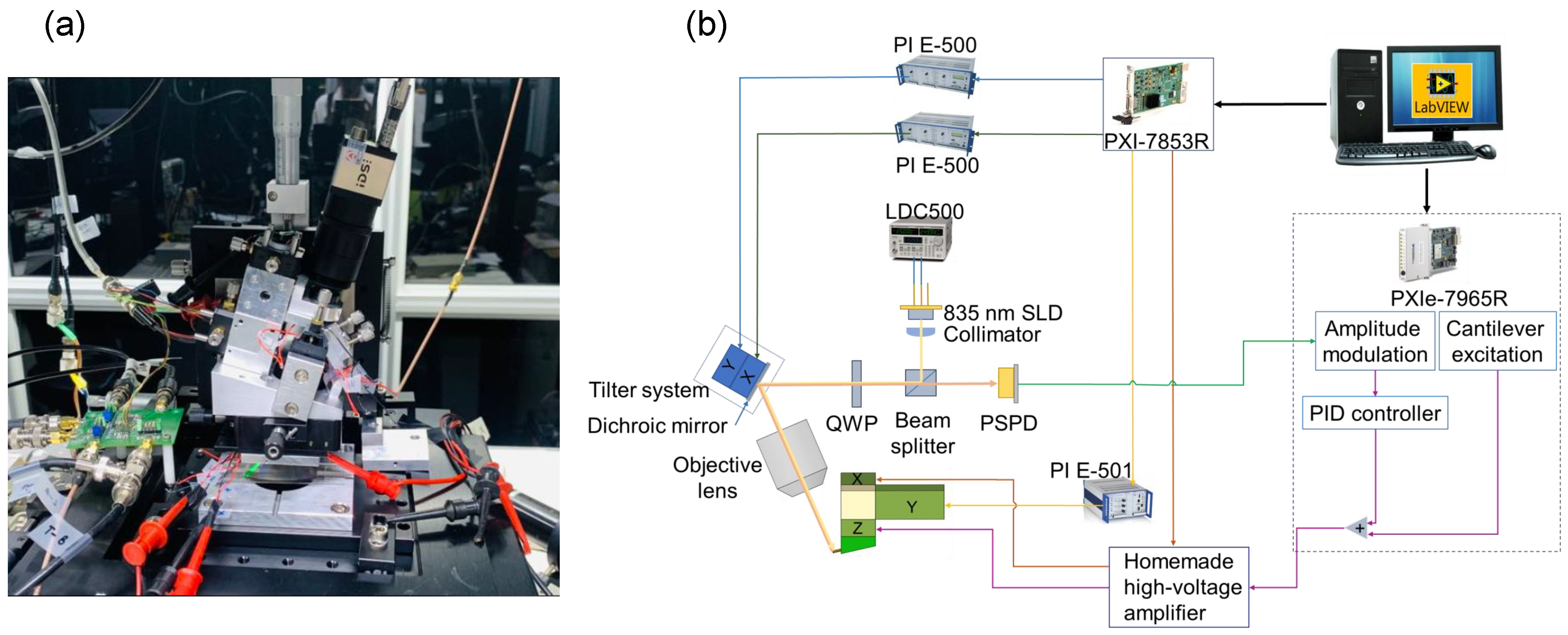
2.1. Experimental Setup

The experiments have been performed with a custom-made tip-scanning AFM system (Figure 1a). Unlike most AFM systems where a sample is mounted on the XY-scanner, our tip-scanning AFM system has an inverted structure. Specifically, a cantilever is mounted on the platform of the XY-scanner while sample remains stationary. As the cantilever moves across the sample surface, a laser tracking system is used to track the cantilever movement, ensuring the laser beam tracks the movement of the cantilever.

Figure 1b illustrates the control diagram of the tip-scanning AFM system. The system uses a tapping mode cantilever (RTESP-300, Bruker, San Jose, CA, USA) with the nominal resonance frequency of 300 kHz, a field programmable gate array (FPGA) module with reconfigurable input/output card (PXI-7856R, National Instruments, Austin, TX, USA), and a flexible reconfigurable input/output (FlexRIO) card (PXIe-7965R, National Instruments, Austin, TX, USA). The PXI-7856R FPGA card is used to generate the drive signals for piezoelectric actuator-driven lateral-direction scanners, while the PXIe-7965R FPGA card is used to receive the signal from the photodiodes, to calculate feedback parameters, and to generate drive signals for the Z-scanner. A 835 nm laser diode is driven by a laser diode controller (LDC500, Stanford Research System, Sunnyvale, CA, USA). Commercial piezo drivers (E-500 and E-501, Physik Instrumente, Karlsruhe, Germany) and a homemade high-voltage amplifier with a small signal bandwidth of 110 kHz are used to drive piezoelectric actuators of the AFM scanners. A software code written with LabVIEW FPGA (LabVIEW 2020, 32-bit, National Instruments, Austin, TX, USA) and Real-Time controls the whole AFM system, recording sample surface information and displaying images. A calibration grating sample with a depth of 200 nanometers and a pitch of 10 µm is utilized in our imaging experiments. All images in this study were obtained in tapping mode with a scan size of about 18 × 18 µm and a resolution of 256 × 256 pixels.

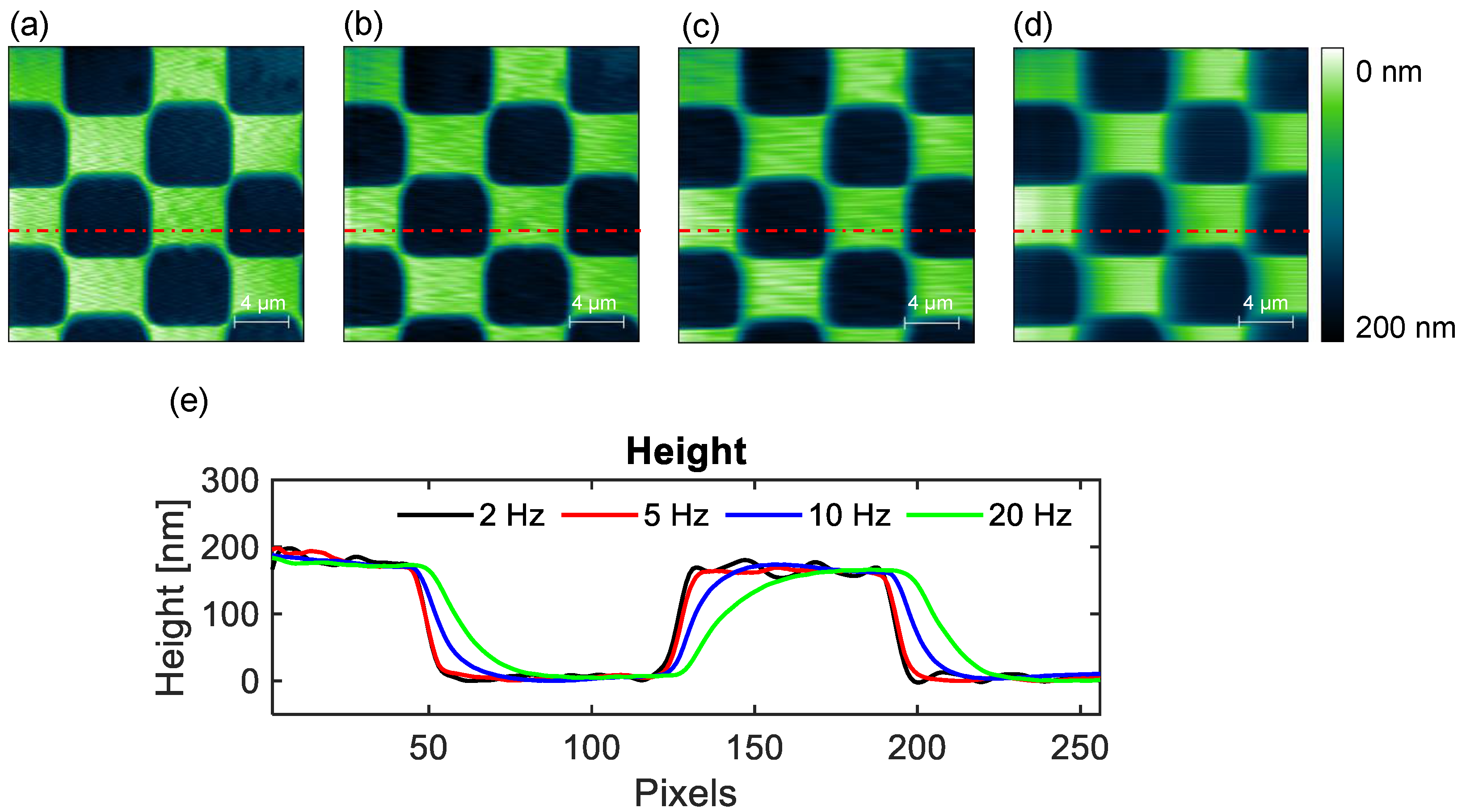
2.2. The Relationship Between Scan Speed and Image Quality

The fixed-speed scanning method is used in most AFM systems today. This approach is simple to implement since AFM maintains a constant scanning speed across all scanning points [24]. However, AFM operators often need to find a balance between two inter-related factors: scan speed and image quality. This is especially important for sample surfaces with high complexity or steep features.

To study the effects of the scan speed on image quality, we conducted AFM scans of the standard calibration grating sample at different fixed speeds. Figure 2a–d show images of the standard calibration grating sample obtained using our AFM system at scanning speeds of 2 Hz, 5 Hz, 10 Hz, and 20 Hz, respectively. The images obtained at low speeds have relatively high sharpness, whereas the image quality captured at higher speeds is lower. At high speeds, the edges of the surface features become significantly blurred. This is typically due to the fact that the speed of the Z-scanner is not fast enough to keep up with the changes in the surface topography in fast scans. The profiles of the marked lines in Figure 2a–d are compared and shown in Figure 2e. A comparison of the line profiles shows that there is not much difference in the image quality obtained at low and high speeds for flat areas. However, the edges of the surface features begin to exhibit decreasing slopes as the scan speed increases. For typical imaging, most AFM operators decrease the scan speed to a sufficiently low value so that the surface features can be tracked by the cantilever. However, operating at a low speed means that the scan time for smooth areas is inefficiently long, since operating at higher scan speeds could still yield good images. Therefore, if there is a way to adjust the scan speed throughout the image acquisition, the scan time can be shortened while the quality of acquired images is not compromised.

Through extensive efforts, variable, adaptive scan speed methods have been studied to enhance the performance of AFM. In [25], a compressive sensing AFM strategy has been proposed to reduce the scan time and improve the image quality. This is a complex method that requires high computation costs due to the need to use the alternating direction algorithm and total variation minimization by an augmented Lagrangian to reconstruct the entire AFM image. In addition, a preliminary scan of the entire sample surface is also required to assess its complexity. Therefore, despite shortening the scan time, this method still requires a considerable amount of computational time. The authors in [26] analyzed the tracking error at each scan point to adjust the scan speed for each point. In their research, the original scan speed in the smooth region is found using the response performance of the feedback controller. In rough areas, the feedback system determines when the tracking error is small enough for the probe to move to the next scan point. Another simple technique using the error signal to improve the imaging speed of AFM has been reported in [27]. Although the scan time has been reduced, these two techniques still have the limitation in which noticeable vibrations are present at the boundaries due to the rapidly changing scan speed. Another adaptive technique using a linear algorithm to increase or decrease the scan speed based on the error signal has been reported in [24]. This technique addresses system vibrations caused by rapidly changing scan speeds. In this method, the system increases the scan speed linearly to the fastest speed when the error is negligible and begins to decrease the scan speed linearly as the error increases, thereby decreasing the overall imaging time by about three times.

We propose a much simpler algorithm to implement compared to the previously reported methods in an attempt to reduce the overall imaging time. Early surface topography prediction allows us to adjust the scan speed mostly in smooth areas, thereby helping to stabilize the system and minimize the unwanted effects due to accelerating or decelerating cantilever motions. Although the overall imaging time is shortened, the image quality is not compromised since rough areas are scanned at a lower speed compared to smooth areas. The details of the proposed algorithm will be further discussed in the next section.

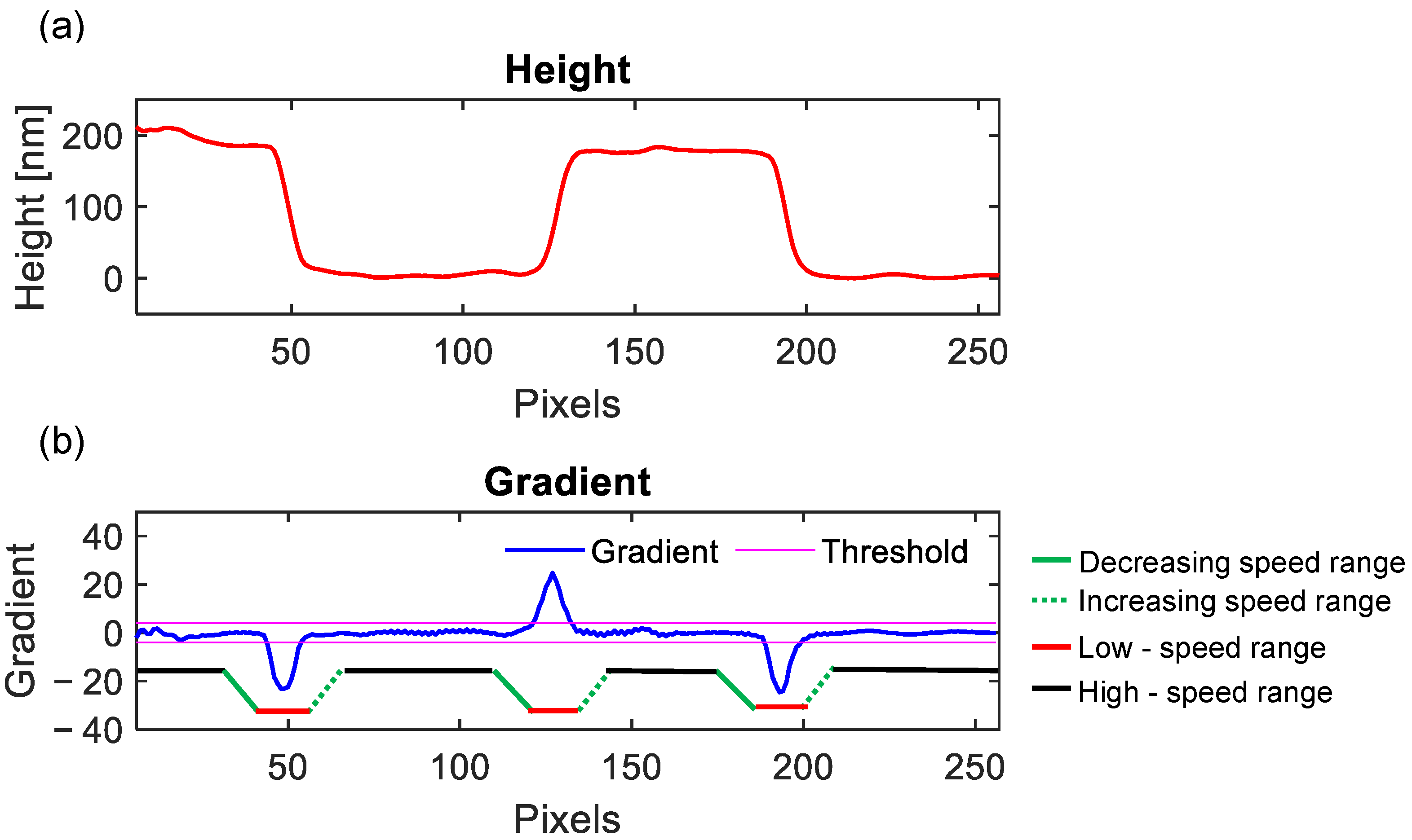
2.3. Real-Time Rate Adaptive Control Algorithm Design

Our proposed algorithm aims to leverage the similarity in topography between neighboring scan lines. The topographic information collected during a line scan will be used to set the scan speed for the successive line scan. Specifically, we use the profile of a previous line scan, calculate and analyze the gradient, and then use the result of the analysis to control the speed of the X-scanner for the present line scan.

In this study, the gradient (G), calculated based on the height difference between two consecutive pixels (Equation (1)), is used to assess the complexity of the sample surface. If the absolute value of the gradient is greater than a preset threshold, that location is considered to be rough while the opposite is considered to be smooth. The threshold is a positive value introduced to minimize the impact of the white noise on the performance of the variable speed control algorithm. Therefore, the more stable the AFM system is, the higher the performance of the variable scan speed algorithm.

$$G=h_k-h_{k+1}$$

(1)

where $h_k$ and $h_{k+1}$ are the heights of sample at the $k^{th}$ and $k+1^{th}$ pixels, respectively.

Figure 3a,b illustrate a line profile in the AFM image obtained at 5 Hz (Figure 2b) and its calculated gradient, respectively. From the graph representing the calculated gradient, we classify the linear range into two types: high-gradient or low-gradient ranges, corresponding to the relatively rough or smooth ranges, respectively. The main point of our proposed algorithm is to employ a fast scan speed in the low-gradient range and a slow scan speed in the high-gradient range. In the transition range around the point where the gradient is equal to the preset threshold, the scan speed either increases or decreases linearly depending on the sign of the gradient, as illustrated in Figure 3b.

The implemented tracking rule for the real-time variable scan speed control algorithm is shown in

Table 1. Tracking rule for the real-time adaptive control algorithm.

	${\mathit{V}}_{\mathit{k}}={\mathit{V}}_{\mathit{min}}$	${\mathit{V}}_{\mathit{min}}<{\mathit{V}}_{\mathit{k}}<{\mathit{V}}_{\mathit{max}}$	${\mathit{V}}_{\mathit{k}}={\mathit{V}}_{\mathit{max}}$
The scanning point is in a rough range or is about to enter a rough range.	$V_k=V_{k+1}$	$V_k=V_k$ − $\Delta V$	$V_k=V_k$ − $\Delta V$
The scanning point is in a smooth range.	$V_k=V_k$ + $\Delta V$	$V_k=V_k$ + $\Delta V$	$V_k=V_{k+1}$

. By comparing the gradient with the threshold of pixels from k to $k+12$ in the preceding line, the speed change direction of the $k^{th}$ pixel in the present line may be ascertained. The system perceives the range as smooth and progressively accelerates if the gradients of the 12 pixels in the preceding row are all below the threshold. The system will progressively slow down if any of these pixels are over the threshold, which denotes a rough range or approaching a rough range.

In our tip-scanning AFM system, the X-scanner is controlled by the software code on the PXI-7856R FPGA card while the surface topographic information from the Z-scanner is processed on the PXIe-7965R FPGA card. First, the topographic information is transferred from the PXIe-7965R card to the PXI-7856R card using DMA FIFO. Then, the gradient of the surface topography is calculated by the PXI-7856R FPGA card and passed through the tracking rule block to adjust the scan speed for each scanning point (Figure 4).

3. Results and Discussion

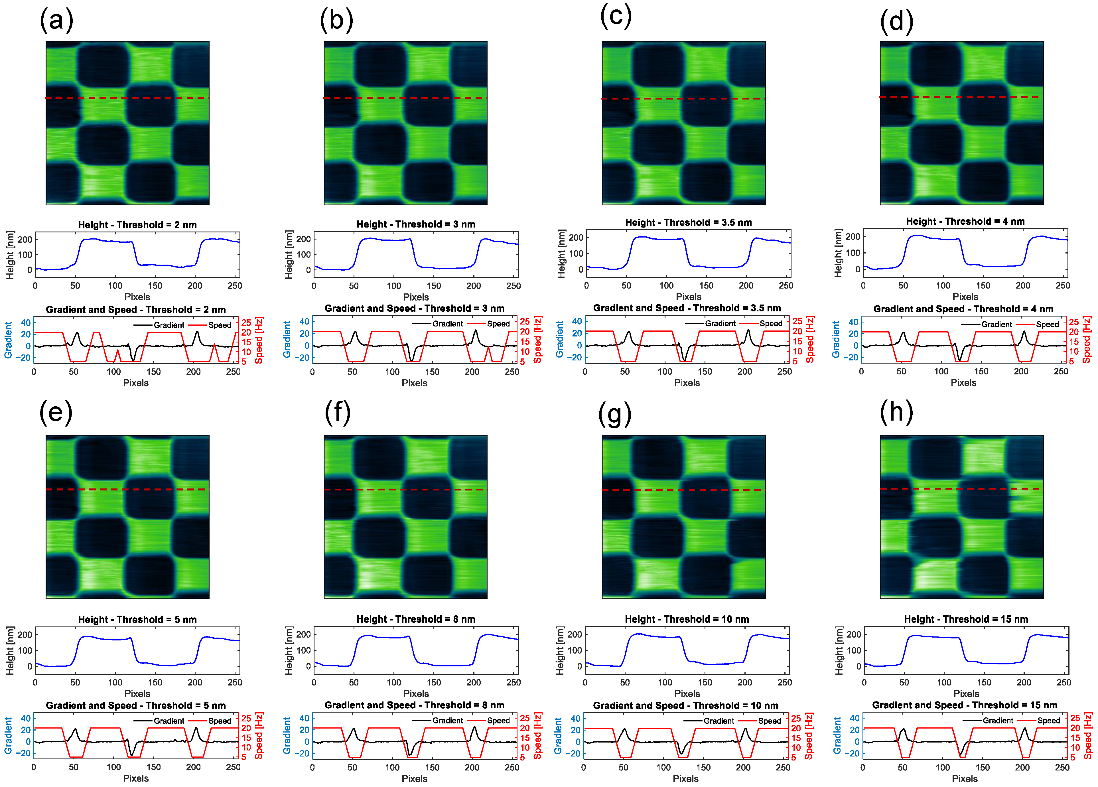
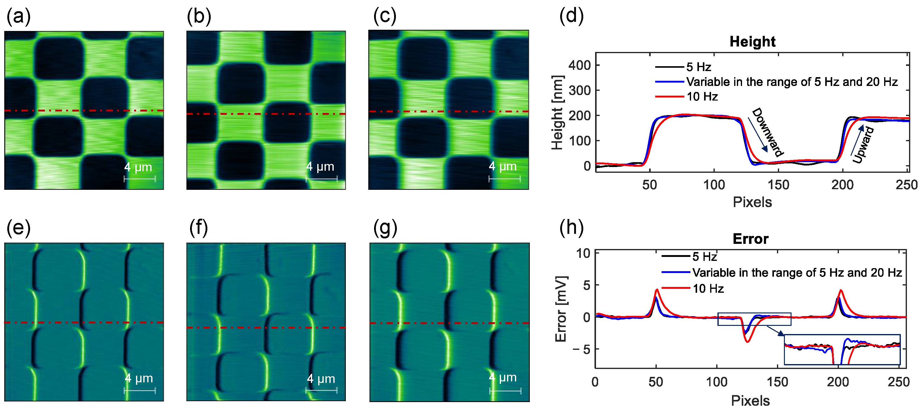
Effectiveness of the Proposed Variable Scan Speed Control Method

The gradient threshold is a critical factor that directly affects the tracking performance of the variable speed control algorithm. In this study, the selection of the gradient threshold is based on two main criteria. First, the threshold must be greater than the measurement error of the system to ensure stable operation and to prevent adaptation to false signals caused by measurement noise. Second, the threshold should be as small as possible, since a smaller threshold makes the system more sensitive to terrain changes and allows better adaptation to even minor variations. Based on these two criteria, we conducted experiments to determine suitable threshold values for the current scanning system.

Figure 5 presents the surface images of the standard calibration sample obtained using the variable speed control algorithm, along with graphs showing height, gradient, and speed at different threshold values. The graph illustrating the relationship between gradient and speed indicates that when the threshold is below 3.5 nm, the algorithm is affected by measurement noise, leading to speed adjustments even in flat regions. Conversely, when the threshold exceeds 8 nm, the algorithm does not respond to small surface variations, causing some details at the edges of features to be missed or inaccurately reconstructed.

Experimental results show that usable threshold values fall within the range of 3.5 nm to 8 nm. However, we prioritize selecting threshold values that do not exceed 3.5 nm by too much, to maintain a balance between the sensitivity of the algorithm and the influence of measurement noise, under the criteria outlined above.

The input parameters for the control algorithm are the minimum speed ($V_{min}$) and the step size ($\Delta V$). The minimum speed is typically pre-determined based on the system calibration. When scanning at some fixed scan speed, reducing the speed below this minimum value should not significantly improve the image quality. The step must be small enough to avoid noticeable oscillations caused by sudden speed changes during scanning. The number of steps required for adjusting the minimum scan speed to the maximum scan speed is set during the algorithm design process. In our demonstration experiments, we used a minimum scan speed of 5 Hz, a step size of 1.5 Hz, and the maximum speed was set to 20 Hz. The threshold was set to 3.5 nm. The gain parameters of the PI (proportional–integral) feedback controller are kept constant throughout the experiment. When sample scanning begins, the first line will always be scanned with the minimum scan speed, and the variable scan speed control process starts with the second line.

The performance of the proposed method is evaluated by comparing the results obtained using a fixed-speed scan method with those obtained using the variable scan speed control method. Figure 6a shows the image acquired at the fixed scan speed of 5 Hz. The total scan time was approximately 52 s. Figure 6b shows the image acquired by using the variable scan speed control method. The total scan time was approximately 22.5 s. This scan time is approximately equal to the time required for imaging at the fixed scan speed of 11.4 Hz. Figure 6c shows the image acquired at the fixed scan speed of 10 Hz with the approximate scan time of 26 s. The edges in the image acquired at 10 Hz clearly appear to be blurred and lack sharpness. However, the image obtained using the variable scan speed control is significantly clearer in spite of the shorter image acquisition time.

Figure 6d displays the surface height profiles along the dashed lines in Figure 6a–c. The line profiles clearly show that the tip fails to accurately follow the sharp changes in topography for the scan speed of 10 Hz. However, the line profile obtained with the variable scan speed control method is nearly identical to that obtained at 5 Hz.

To evaluate the effectiveness of the adaptive speed control method, the slopes at the rising and falling edges marked in Figure 6d are also calculated and presented in

Table 2. Comparison of performance between the variable scan speed method and the fixed scan speed method.

		Fixed Scan Speed (5 Hz)	Variable Scan Speed (Equivalent to 11.4 Hz)	Fixed Scan Speed (10 Hz)
Time [s]		52	22.5	26
Slope of downward edge		−15.79	−13.63	−6.98
Slope of upward edge		17.16	17.05	8.19
MSE [mV]		13.56	14.49	42.82

. The slopes at the falling and rising edges are −6.98 and 8.19, respectively, for the fixed scan speed of 10 Hz. The slopes at the same two edges are −13.63 and 17.05 for the image obtained with the adaptive speed control. Since a higher value for the slope means that the vertical feedback is better tracking surface features, our implementation of the proposed control is successfully reducing the scan speed for rough ranges to allow better surface tracking. This is also confirmed by the fact that the values of the slopes calculated from the image obtained with the adaptive scan speed control are close to the values calculated from the image obtained at the fixed scan speed of 5 Hz.

To provide additional evidence for the successful implementation of the proposed variable scan speed control method, the tracking error has also been included in the analysis. Figure 6e–g show the error signal images obtained with the fixed scan speed of 5 Hz, the variable scan speed control, and the fixed scan speed of 10 Hz, respectively. As shown in Figure 6h, the comparison of the line profiles along the marked lines in the error signal images demonstrates that the variable scan speed control can successfully match the level of error signal achieved at a slow scan speed while the overall scan time is reduced to match that for a fast scan speed. The mean square error (MSE) values for the investigated cases were calculated and presented in Table 2. Although the scan speed is equivalent to about 11.4 Hz, the calculated MSE is significantly smaller than the calculated value for the fixed scan speed of 10 Hz and comparable to the calculated value for the fixed scan speed of 5 Hz. These results successfully demonstrate that the proposed algorithm is able to combine both high-quality imaging and a short imaging time, which is typically impossible for rough topographic samples at a fixed scan speed.

To assess the effectiveness of the system in adjusting the scanning speed according to the change in surface topography, we recorded the scan speed at each scan point and analyzed its correlation with height variations. In particular, Figure 6b is selected; three lines have been marked and presented in Figure 7a to assist in analyzing the tracking performance of the AFM system. Figure 7b–d show the corresponding line profiles for the three lines marked in Figure 7a along with the scan speed in Hz and the calculated gradient. The results indicate that the system operates successfully at a high scan speed in smooth ranges and at a low scan speed in rough ranges. It is also clear that the system either slows down or speeds up before either approaching or leaving a rough range, adhering to the tracking rule established in our design.

4. Conclusions

In this research, we have successfully designed and implemented a variable scan speed control algorithm. The proposed algorithm leverages the similarity in topography between two successive scan lines and uses the topographic information from the previous line to adjust the scan speed for the following line. Our experimental results indicate that for a certain sample, it is possible to reduce the scan time by 50% or more compared to a fixed single speed scan with similar imaging quality. In conclusion, we have successfully presented a method to shorten the time required for imaging without significantly sacrificing image quality by adjusting scan speed in real-time.

References

1. Binnig, G.; Quate, C.F.; Gerber, C. Atomic force microscope. Phys. Rev. Lett. 1986, 56, 930. [Google Scholar] [CrossRef]
2. Suzuki, Y.; Sakai, N.; Yoshida, A.; Uekusa, Y.; Yagi, A.; Imaoka, Y.; Takeyasu, K. High-speed atomic force microscopy combined with inverted optical microscopy for studying cellular events. Sci. Rep. 2013, 3, 2131. [Google Scholar] [CrossRef]
3. Liu, L.; Kong, M.; Wu, S.; Xu, X.; Wang, D. Error Analysis of the Combined-Scan High-Speed Atomic Force Microscopy. Sensors 2021, 21, 6139. [Google Scholar] [CrossRef]
4. Viani, M.B.; Schäffer, T.E.; Chand, A.; Rief, M.; Gaub, H.E.; Hansma, P.K. Small cantilevers for force spectroscopy of single molecules. J. Appl. Phys. 1999, 86, 2258–2262. [Google Scholar] [CrossRef]
5. Fantner, G.E.; Schitter, G.; Kindt, J.H.; Ivanov, T.; Ivanova, K.; Patel, R.; Hansma, P.K. Components for high speed atomic force microscopy. Ultramicroscopy 2006, 106, 881–887. [Google Scholar] [CrossRef]
6. Fukuda, S.; Uchihashi, T.; Iino, R.; Okazaki, Y.; Yoshida, M.; Igarashi, K.; Ando, T. High-speed atomic force microscope combined with single-molecule fluorescence microscope. Rev. Sci. Instrum. 2013, 84, 073706. [Google Scholar] [CrossRef]
7. Umakoshi, T.; Fukuda, S.; Iino, R.; Uchihashi, T.; Ando, T. High-speed near-field fluorescence microscopy combined with high-speed atomic force microscopy for biological studies. BBA-Gen. Subj. 2020, 1864, 129325. [Google Scholar] [CrossRef]
8. Qiu, Y.; Sajidah, E.S.; Kondo, S.; Narimatsu, S.; Sandira, M.I.; Higashiguchi, Y.; Wong, R.W. An Efficient Method for Isolating and Purifying Nuclei from Mice Brain for Single-Molecule Imaging Using High-Speed Atomic Force Microscopy. Cells 2024, 13, 279. [Google Scholar] [CrossRef]
9. Watanabe, H.; Uchihashi, T. Development of Wide-area Tip-scanning High-speed Atomic Force Microscopy. In Proceedings of the 2019 IEEE the International Conference on Manipulation, Manufacturing and Measurement on the Nanoscale (3M-NANO), Zhenjiang, China, 4–8 August 2019; pp. 281–285. [Google Scholar]
10. Uchihashi, T.; Watanabe, H.; Fukuda, S.; Shibata, M.; Ando, T. Functional extension of high-speed AFM for wider biological applications. Ultramicroscopy 2016, 160, 182–196. [Google Scholar] [CrossRef]
11. Wadikhaye, S.P.; Yong, Y.K.; Reza Moheimani, S.O. A serial-kinematic nanopositioner for high-speed atomic force microscopy. Rev. Sci. Instrum. 2014, 85, 105104. [Google Scholar] [CrossRef]
12. Schitter, G.; Thurner, P.J.; Hansma, P.K. Design and input-shaping control of a novel scanner for high-speed atomic force microscopy. Mechatronics 2008, 18, 282–288. [Google Scholar] [CrossRef]
13. Humphris, A.D.L.; Miles, M.J.; Hobbs, J.K. A mechanical microscope: High-speed atomic force microscopy. Appl. Phys. Lett. 2005, 86, 034106. [Google Scholar] [CrossRef]
14. Fukuma, T.; Okazaki, Y.; Kodera, N.; Uchihashi, T.; Ando, T. High resonance frequency force microscope scanner using inertia balance support. Appl. Phys. Lett. 2008, 92, 243119. [Google Scholar] [CrossRef]
15. Ando, T.; Uchihashi, T.; Fukuma, T. High-speed atomic force microscopy for nano-visualization of dynamic biomolecular processes. Prog. Surf. Sci. 2008, 83, 337–437. [Google Scholar] [CrossRef]
16. Ando, T.; Kodera, N.; Takai, E.; Maruyama, D.; Saito, K.; Toda, A. A high-speed atomic force microscope for studying biological macromolecules. Proc. Natl. Acad. Sci. USA 2001, 98, 12468–12472. [Google Scholar] [CrossRef]
17. Miyata, K.; Usho, S.; Yamada, S.; Furuya, S.; Yoshida, K.; Asakawa, H.; Fukuma, T. Separate-type scanner and wideband high-voltage amplifier for atomic-resolution and high-speed atomic force microscopy. Rev. Sci. Instrum. 2013, 84, 043705. [Google Scholar] [CrossRef]
18. Kenton, B.J.; Leang, K.K. Design and control of a three-axis serial-kinematic high-bandwidth nanopositioner. IEEE-ASME Trans. Mechatron. 2011, 17, 356–369. [Google Scholar] [CrossRef]
19. Yong, Y.K.; Bhikkaji, B.; Moheimani, S.R.R. Design, modeling, and FPAA-based control of a high-speed atomic force microscope nanopositioner. IEEE-ASME Trans. Mechatron. 2012, 18, 1060–1071. [Google Scholar] [CrossRef]
20. Schitter, G.; Menold, P.; Knapp, H.F.; Allgöwer, F.; Stemmer, A. High performance feedback for fast scanning atomic force microscopes. Rev. Sci. Instrum. 2001, 72, 3320–3327. [Google Scholar] [CrossRef]
21. Bhikkaji, B.; Moheimani, S.R. Integral resonant control of a piezoelectric tube actuator for fast nanoscale positioning. IEEE/ASME Trans. Mechatron. 2008, 13, 530–537. [Google Scholar] [CrossRef]
22. Wadikhaye, S.P.; Yong, Y.K.; Bhikkaji, B.; Moheimani, S.R. Control of a piezoelectrically actuated high-speed serial-kinematic AFM nanopositioner. Smart Mater. Struct. 2014, 23, 025030. [Google Scholar] [CrossRef]
23. Fantner, G.E.; Hegarty, P.; Kindt, J.H.; Schitter, G.; Cidade, G.A.; Hansma, P.K. Data acquisition system for high speed atomic force microscopy. Rev. Sci. Instrum. 2005, 76, 026118. [Google Scholar] [CrossRef]
24. Zhang, Y.; Li, Y.; Shan, G.; Chen, Y.; Wang, Z.; Qian, J. Real-time scan speed control of the atomic force microscopy for reducing imaging time based on sample topography. Micron 2018, 106, 1–6. [Google Scholar] [CrossRef]
25. Han, G.; Chen, Y.; Wu, T.; Li, H.; Luo, J. Adaptive AFM imaging based on object detection using compressive sensing. Micron 2022, 154, 103197. [Google Scholar] [CrossRef]
26. Wang, Y.; Wan, J.; Hu, X.; Xu, L.; Wu, S.; Hu, X. A rate adaptive control method for improving the imaging speed of atomic force microscopy. Ultramicroscopy 2015, 155, 49–54. [Google Scholar] [CrossRef]
27. Ahmad, A.; Schuh, A.; Rangelow, I.W. Adaptive AFM scan speed control for high aspect ratio fast structure tracking. Rev. Sci. Instrum. 2014, 85, 103706. [Google Scholar] [CrossRef]
Figure 1. (a) Tip-scanning AFM system and (b) its control diagram.
Actuators 14 00262 g001
Figure 2. Tapping mode images of the calibration grating obtained at various scan speeds: (a) 2 Hz, (b) 5 Hz, (c) 10 Hz, and (d) 20 Hz. The line profiles for the marked lines in (ad) are shown in (e).
Actuators 14 00262 g002
Figure 3. (a) The profile of the marked line in the image obtained at 5 Hz (Figure 2b) and (b) its gradient.
Actuators 14 00262 g003
Figure 4. The process of transmitting topography information.
Actuators 14 00262 g004
Figure 5. Tapping mode images of a calibration grating sample obtained using the variable speed control along with graphs of its height, gradient, and speed along the marked line, corresponding to threshold values of (a) 2 nm, (b) 3 nm, (c) 3.5 nm, (d) 4 nm, (e) 5 nm, (f) 8 nm, (g) 10 nm, and (h) 15 nm.
Actuators 14 00262 g005
Figure 6. Tapping mode images and their corresponding error images of the standard calibration grating sample obtained at different scan speeds: (a,e) at the fixed scan speed of 5 Hz (52 s), (b,f) with the variable scan speed (22.5 s), and (c,g) at the fixed scan speed of 10 Hz (26 s). The time shown in parenthesis denotes the image acquisition time. The comparison of the surface profiles along the marked lines in (ac) is shown in (d). The comparison of the error signals along the marked lines in (eg) is shown in (h).
Actuators 14 00262 g006
Figure 7. (a) Tapping mode images of a calibration grating sample using the variable speed control (equivalent to a fixed scan speed of 11.4 Hz). Line profiles, scan speed, and gradient for (b) Line 53, (c) Line 142, and (d) Line 198.
Actuators 14 00262 g007