Neural Network and Generalized Extended State Observer Sliding Mode Control of Hydraulic Cylinder Position in the Independent Metering Control System with Digital Valves

Abstract

The independent metering control system is renowned for its ability to independently regulate the flow and pressure of various actuators, achieving high efficiency and energy savings in hydraulic systems. The high-speed digital valve is known for its fast response to control signals and precise fluid control. However, challenges such as jitter in the position control of hydraulic cylinders, unknown dead zone nonlinearity, and time variance in electro-hydraulic proportional systems necessitate further investigation. To address these issues, this study initially establishes an independent metering control system with digital valves. Based on the state space equation and Lyapunov stability judgment conditions, a high-order sliding mode controller is designed. In addition, a radial basis function (RBF) neural network is constructed to approximate uncertainties arising from the modeling process, the accuracy error indicator uses Mean Absolute Error (MAE), and a finite time generalized extended state observer (GESO) is introduced to conduct online disturbance observation for the external disturbances present within the control system. Consequently, a variable structure high-order sliding mode control strategy, augmented by RBF neural networks and finite time generalized extended state observer (RBF-GESO-SMC), is proposed. Finally, simulations and experimental verification are performed, followed by a comprehensive analysis of the experimental results. Compared with the sliding mode control (SMC), the RBF-GESO-SMC diminishes the displacement-tracking control accuracy error by 63.7%. Compared with traditional Proportional-Integral-Derivative (PID) control, it reduces the displacement-tracking control accuracy error by 78.1%. The results indicate that, through the comparison with SMC and PID control, RBF-GESO-SMC exerts significant influence on the improvement of position accuracy, anti-interference ability, transient response performance, and stability.

1. Introduction

The traditional hydraulic system adopts centralized valve control, with multiple actuators sharing the same valve group, which has problems such as high energy loss and action interference. With the development of electronic control technology and energy-saving needs, independent metering systems (IMSs) have emerged [1,2,3]. By equipping each actuator (hydraulic cylinder, motor, etc.) with independent valve groups and sensors, flow and pressure can be accurately regulated, solving the efficiency and flexibility bottlenecks of traditional systems [4,5]. IMS is widely used in construction machinery, such as excavators and cranes, to reduce fuel consumption by independently controlling the actions of the boom, bucket, etc., combined with energy recovery technology, thus realizing high-precision pressure control in industrial equipment (injection molding machines, machine tools) to improve product quality. The aerospace industry utilizes its redundant design to enhance reliability. In addition, IMS optimizes energy utilization efficiency in the field of new energy (wind power variable pitch, wave energy generation). This system can save more than 30% energy and has the advantages of fast response and flexible operation, promoting the transformation towards intelligent and green hydraulic technology [6,7].

With the continuous advancement of modern industrial automation, hydraulic drive systems have become widely adopted across various fields, attributed to their high power density and excellent dynamic performance. At present, digital valves are extensively utilized in heavy machinery, aerospace, military equipment, and other critical domains [8,9,10,11,12]. A hydraulic cylinder serves as the core actuator in the hydraulic drive system, with the precision and response speed of its position control directly affecting the performance and stability of the entire system. However, the traditional digital valve primarily relies on the incremental digital valve as the main operative component, thereby resulting in problems such as core control components’ susceptibility to damage, heightened sensitivity to oil cleanliness and substantial volume, etc. [13]. Moreover, in scenarios where precision requirements are less stringent and cost control is a priority, incremental digital valves may not represent the optimal choice. High-speed on-off valves can be used as an alternative to digital valves.

The management of high-speed digital switching valves necessitates mutual interaction among different tempering signals. The commonly employed modulation signals include pulse width modulation (PWM), pulse number modulation (PNM), and pulse code modulation (PCM) [14,15,16]. Numerous scholars at home and abroad have explored the utilization of high-speed on-off valves for controlling hydraulic cylinder displacement. Reference [17] presented a pre-excitation control algorithm, achieving an 80.0% increase in the linear area of the flow characteristics and a 23% reduction in the adjustment time of the HSV control system. Reference [18] realized compound control of hydraulic cylinder speed and pressure, leveraging a reverse step method within high-speed on-off valves, which contributes to the enhancement of position tracking accuracy. Reference [19] introduced a hydraulic stepping drive technology based on a high-speed on-off valve set and two miniature plunger cylinders. At a load of 3 KN, the drive, with a stroke of 50 μm, exhibited an 11.58% reduction in maximum error. Reference [20] substituted the check valve with two digital valves to facilitate asymmetric flow compensation, thereby enabling high-precision control of hydraulic cylinder displacement. In order to analyze the position control of hydraulic cylinders governed by high-speed switch valves and ensure precise positioning, Reference [21] proposed a composite algorithm of PD, velocity feedforward displacement feedback, and pulse width modulation (PWM) control. Reference [22] adopted a parallel digital valve with a servo valve group and a hydraulic system combined with the sliding mode control strategy. This arrangement not only maintained the uniformity of switching between valves but also effectively controlled the displacement of the spool of the slide valve.

The aforementioned research on the control of hydraulic cylinder displacement, mediated by a digital valve, predominantly uses diverse signal modulation schemes in conjunction with the rapid response speed and high flow accuracy of high-speed on-off valves, with the objective of a broad range of adjustable flow outputs, ultimately facilitating precise control of the actuator position. Nevertheless, due to the inherent binary nature of high-speed on-off valves, flow or pressure pulsations will inevitably induce vibrations in the hydraulic cylinder. Furthermore, proportional electro-hydraulic systems exhibit intricate nonlinear attributes [23], and the commonly deployed proportional valve demonstrates extreme sensitivity to oil, triggering time variance system behavior [24]. When employing PID control, accurately capturing the nonlinear traits of the hydraulic system proves challenging; moreover, in the presence of external disturbances and large-scale displacement adjustments, this approach yields subpar system responses, which potentially undermines both position control precision and overall system stability.

The main principle of sliding mode structure control technology centers on the design of a stable sliding surface that directs the system towards and along the sliding surface to reach the origin, enabling rapid convergence to the desired state [25]. The sliding mode control (SMC) technology embodies a discontinuous nonlinear control technology that is impervious to the parameters of the controlled object or the operational environment. In response to the intricacies of motion disturbance and low loading accuracy in electro-hydraulic load simulation systems, Reference [26] introduced a sliding mode self-disturbance rejection composite controller, which can markedly diminish system chattering, solve problems of fixed-time convergence, and augment system loading performance and disturbance rejection. Additionally, in order to enhance the force control performance and anti-interference robustness of the electro-hydraulic servo material testing machine, Reference [27] proposed an integral sliding film control method predicated on feedback linearization, thereby achieving high-precision tracking of the machines’ force control system. Moreover, to mitigate the impact of unknown disturbances on the control performance of hydraulic servo systems, Reference [28] presents a sliding mode variable structure control utilizing space vector adjustment technology. Experimental validations underscore that this designed controller proficiently suppresses the influence of large system disturbances, enhancing both the control accuracy and system response dynamics. Although the above research results have strong robustness to the composite interference caused by internal parameter changes and external disturbances in the system, they all elucidate proposed constraints.

In the domain of control science, controller design is prone to be constrained by modeling techniques. Mathematical models established based on actual systems are frequently accompanied by unpredictability in controlled object, including parameter uncertainty, and uncertainties in nonlinear unknown functions, complicated structures, and unmodeled dynamics. To address these issues, neural network control is a highly effective tool for system manipulation. Reference [29] used an RBF neural network for situation estimation without the need for prior knowledge of uncertainties, ensuring that the robotic arm system converges with a finite time error. For electro-hydraulic servo systems, Reference [30] proposed the combination of a nonlinear neural network (NN) and error sign continuous robust integral (RISE) feedback controller, enabling online parameter updates and asymptotic stability of the system. Reference [31] introduced an extended state observer, which equates the uncertainty and external disturbances in digital hydraulic cylinders to integrated disturbances and employs neural network model reference adaptive control for disturbance rejection. Concerning the difficulty in drift estimation of navigation marks, Reference [32] designed a fractional gradient based on momentum RBF neural network (FOGDM-RBF); and through confirmation of its convergence, it was used for estimating the drift trajectory of navigation marks across diverse geographical locations. Furthermore, to realize more accurate tracking, Reference [33] designed a robust adaptive RBF neural network compensator to approximate and compensate for TDE errors, ensuring the asymptotic stability of the system according to the Lyapunov criterion. Reference [34] proposed several novel hybrid adaptive neural fuzzy inference system methods as prediction models for estimating the downstream scour depth of gates. By removing some prediction variables, three input variable combinations were prepared to obtain a reliable prediction model. 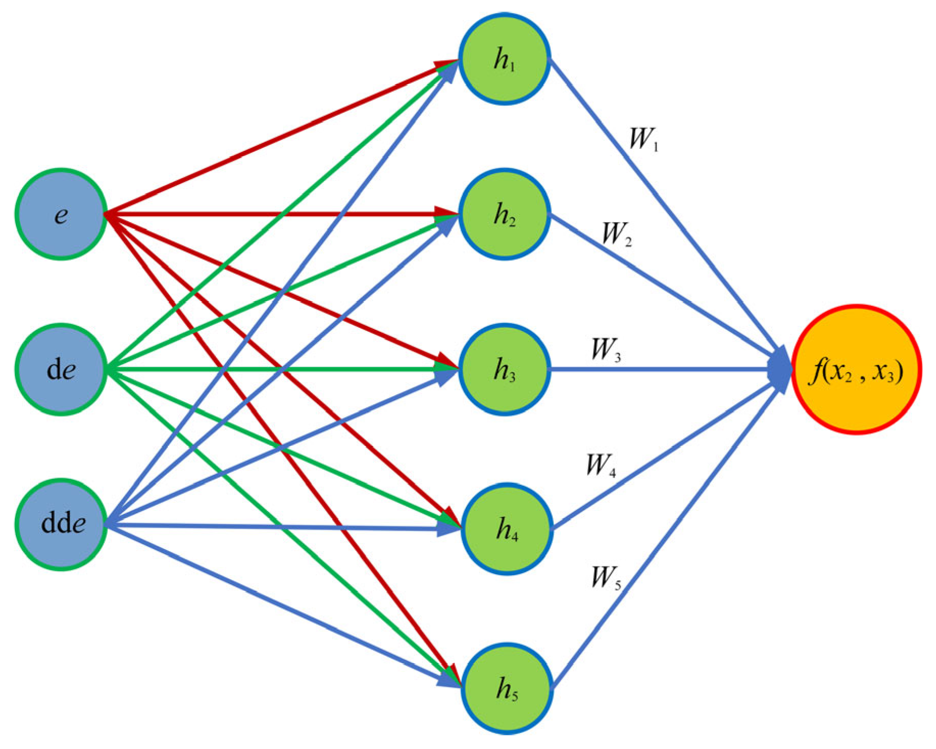Reference [35] demonstrated the application of an adaptive neural fuzzy inference system (ANFIS) combining particle swarm optimization, ant colony optimization, differential evolution, and genetic algorithm. The prediction performance and related uncertainties of scour depth under different scour conditions, including active beds and clean water, were evaluated. The uncertainty results showed that it was related to both the model structure and the combination of input variables. The RBF neural network, through the local response characteristics of radial basis functions, can achieve efficient nonlinear approximation with fewer hidden layer nodes. Compared with traditional fully connected networks (such as the BP network), it has a faster training speed and more stable convergence, making it especially adept at handling data with significant local features and dynamic system modeling. RBF neural network control has higher structural parallelism, efficient computing power, and the ability to preserve system information through neurons and neural weights.

The extended state observer (ESO) excels in estimating and compensating for system disturbances without relying on the specific model of the research object and disturbance. This capability significantly alleviates the negative effects of disturbances on controller performance, making it an indispensable tool adopted in high-precision control exploration of electro-hydraulic position servo systems [36,37]. In order to address the challenges of uncertainty, nonlinearity, and interference in robots, Reference [38] proposed an integrated sliding mode control (ISMC) based on multi input multi output ESO, which effectively solves the problems of uncertainty, nonlinearity, and interference in robotic systems through disturbance estimation and active compensation, dynamic sliding mode surface design, and low gain switching. Concurrently, a formation control strategy utilizing a linear extended state observer (LESO) and an estimated minimum learning parameter (EMLP) neural network was proposed in Reference [39] to address the issues of wind influence and model uncertainty. An adaptive controller based on LESO was designed to monitor and counteract system disturbances, thereby maintaining stability and accuracy of the entire formation flight system. In the context of unmanned surface vehicles (USVs) striving for high-precision trajectory tracking, Reference [40] presented a control strategy using predetermined time tracking control technology and established a predetermined time extended state observer to promptly and accurately reconstruct unmeasurable velocities and lumped disturbances, with the aim to monitor swift error convergence within the designated timeframe. Given their profound effectiveness at mitigating disturbance impacts on the controlled system, extended state observers have garnered widespread adoption within electro-hydraulic servo systems.

In order to tackle existing problems, this paper offers a digital valve-controlled hydraulic cylinder position control method that incorporates load port neural network sliding mode control. The variable structure sliding mode controller deployed in this method exhibited superior performance in regulating the hydraulic system with high-order nonlinear strong coupling and external interference. For the streamlining of the hydraulic control system model, the neural network algorithm with self-learning and self-adapting ability is integrated, which simplifies the hydraulic system model and notably enhances its control properties. The conventional valve-controlled hydraulic system relies on the direction valve to reverse hydraulic systems with the presence of throttling loss in the oil inlet and outlet, which in turn leads to the substantial energy consumption and compromised efficiency of the whole system. Based on this, this paper adopts the independent load port as the hydraulic control system [41,42].

The asymmetric hydraulic cylinder with differing structural parameters in its two cavities makes the modeling process complex. For the previous research on the digital valve-controlled hydraulic cylinder, the symmetric cylinder was mainly utilized as the control object. This paper simplifies the mathematical model based on the existing model of the digital valve-controlled asymmetric hydraulic cylinder.

In this study, the mathematical model of the hydraulic cylinder system is first established, and then analysis of its nonlinear characteristics and disturbance effects is performed to streamline the system. Subsequently, the high-order sliding mode controller in conformity with the provisions of sliding mode control is devised. With the assistance of the simplified model, the radial basis neural network is introduced to approximate the uncertainty aspect of the model online. Finally, the output of the controller is converted into signals that can be effectively used by high-speed switches. The efficacy of the proposed method is verified through simulation and experiment. As shown in the results, the proposed control strategy can significantly improve the accuracy, system response speed, and stability of hydraulic cylinder position control while exhibiting excellent robustness and adaptability under complex load and disturbance conditions.

The main contributions of this research can be categorized into the following three aspects:

• An innovative sliding mode control method is incorporated for the independent metering control system. The RBF neural network and generalized extended state observer are introduced into the model reference adaptive controller, which significantly enhances the accuracy and robustness of position tracking control.
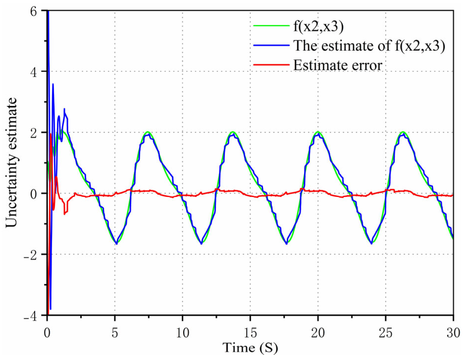
• The adaptive algorithm of the RBF neural network is proposed, with the parameter uncertainty terms estimated and compensated for through the online approximation of unknown matching parameters and the rectification of adaptive control law.
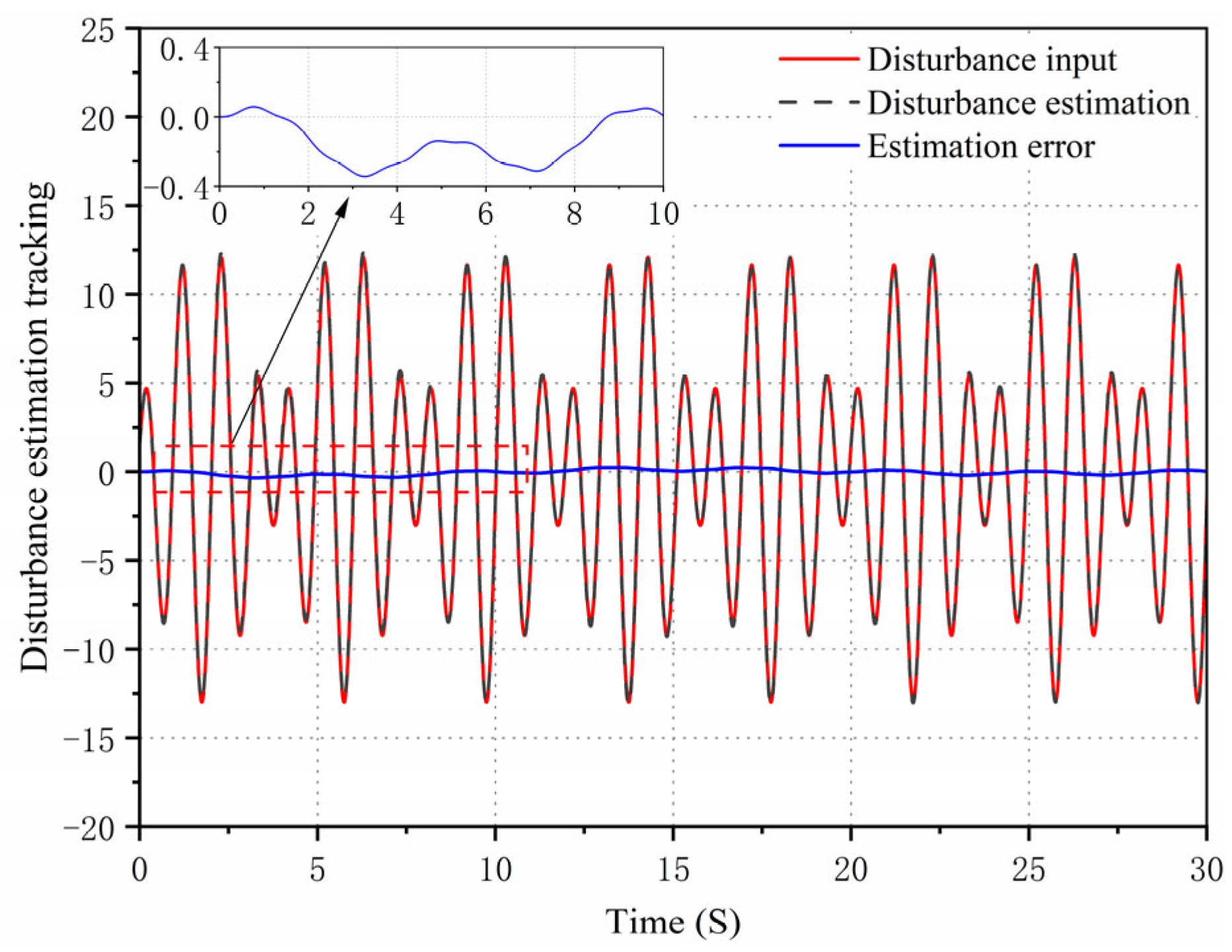
• A finite time generalized extended state observer is designed for real-time monitoring of external disturbances, and the observed values are delivered to the controller to inhibit high gain feedback in the control system.

The structure of this paper is outlined as follows: The Section 2 focuses on the independent metering control system of digital valves and establishes a hydraulic system model. The Section 3 introduces the design of the sliding mode controller based on the RBF neural network and generalized extended state observer in accordance to the hydraulic system model of the digital valve. The Section 4 mainly illustrates the establishment of the simulation model and provides a thorough analysis of the simulation results. The Section 5 constructs an independent metering control system experimental platform with digital valves and compares the control performance of the experiment. The Section 6 summarizes the key findings and contributions of this research.

2. Independent Metering Control System with Digital Valves

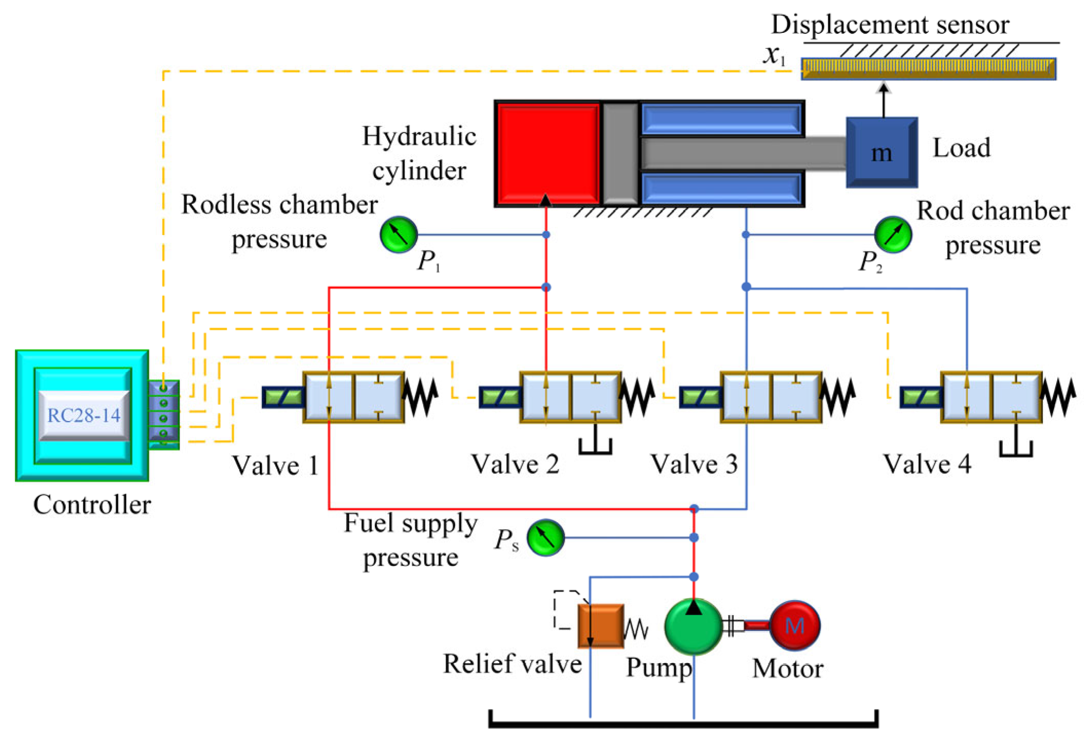
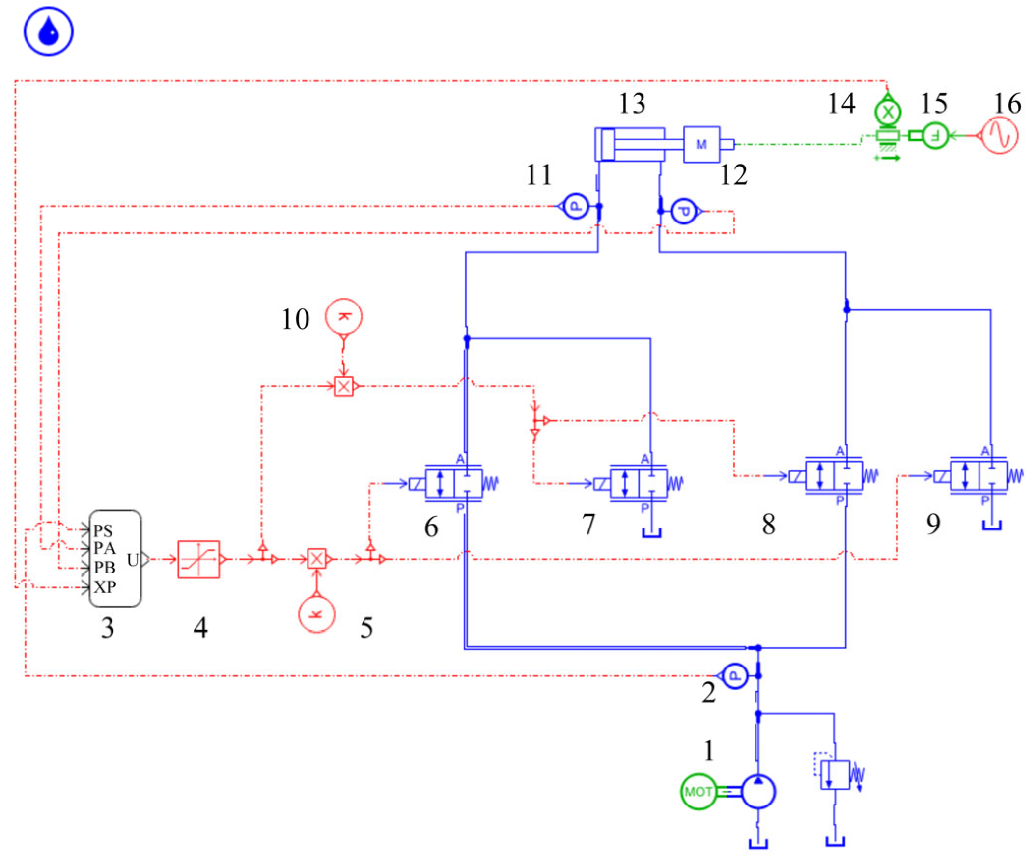
The position control principle for the digital valve-controlled hydraulic cylinder based on an independent metering control system is shown in Figure 1. This includes motors, oil pumps, asymmetric hydraulic cylinders, displacement and pressure sensors, and controllers.

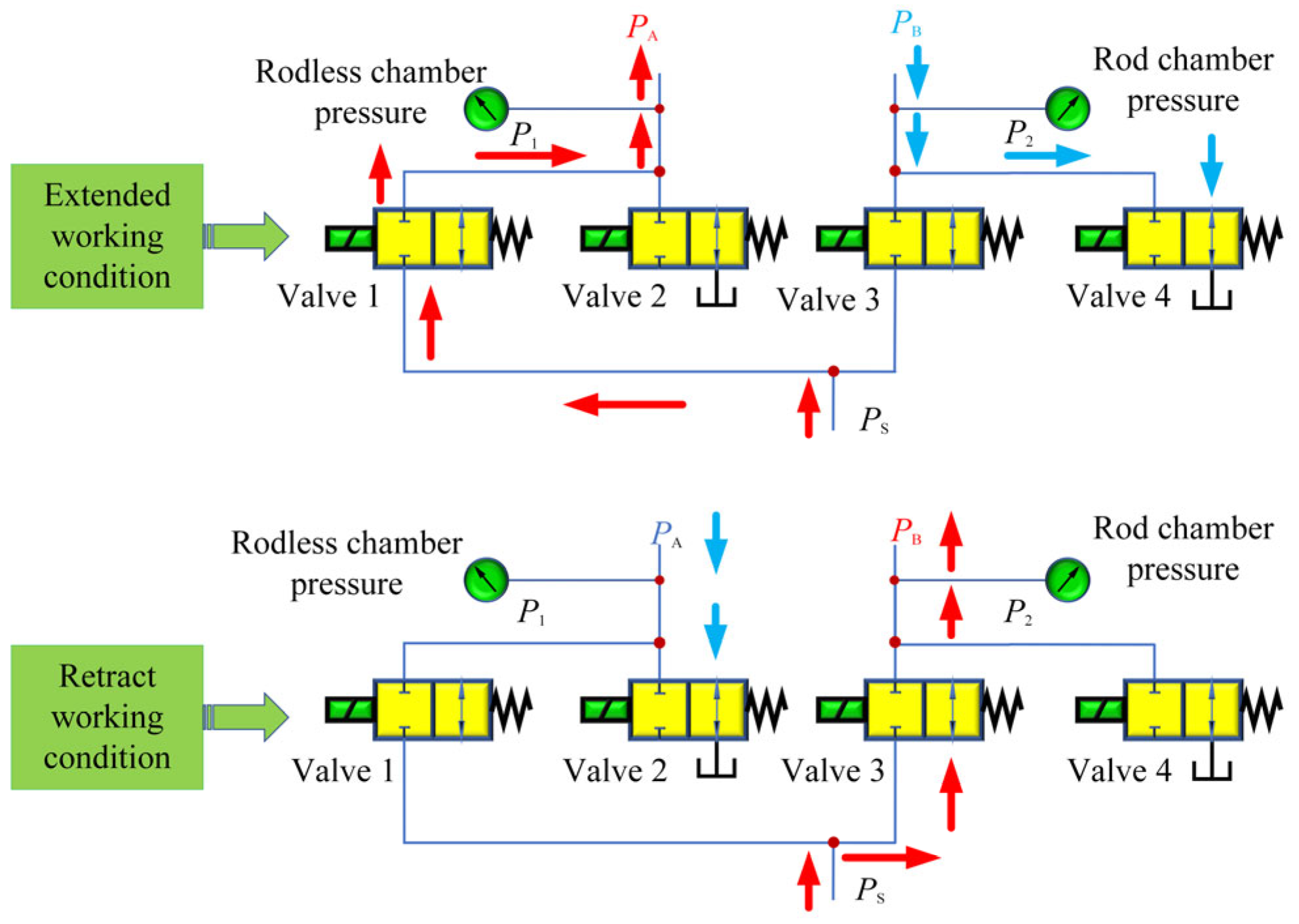
When the high-speed on-off valve 1 and 4 work at the same time, the high-pressure oil will enter from the rodless chamber of the asymmetrical hydraulic cylinder and flow back to the tank through the high-speed on-off valve 4. When the high-speed on-off valves 2 and 3 work at the same time, the high-pressure oil will enter from the rod chamber of the asymmetric hydraulic cylinder and flow back to the tank through the high-speed on-off valve 2. At the same time, the rod chamber pressure gauge will detect the working pressure and play a role in detecting pressure fluctuation. Only two solenoid valves can be powered simultaneously under any operating conditions, as shown in Figure 2.

The process of establishing a mathematical model for the above hydraulic system is as follows:

• It is assumed that $P_s$ is a constant-pressure source supplying oil to the system at a pressure of $P_s$.
• Hydraulic cylinders do not consider motion resistance and friction during their movement.
• It is assumed that the hydraulic oil is incompressible.

The analysis object of the hydraulic system is an asymmetric hydraulic cylinder, and the effective area ratio of the two cavities of the hydraulic cylinder is assumed to be $A_1=\eta A_2$.

The flow rate through the valve port can be expressed by the following formula:

$$Q_1=\left\{\begin{array}{c}{C_{dv}A}_{dv}\sqrt{{\displaystyle \frac{2\left(P_s-P_1\right)}{\rho }}} ,if u\ge 0\\ {C_{dv}A}_{dv}\sqrt{{\displaystyle \frac{2\left(P_1-P_0\right)}{\rho }}} ,if u<0\end{array}\right.$$

(1)

$$Q_2=\left\{\begin{array}{c}{C_{dv}A}_{dv}\sqrt{{\displaystyle \frac{2\left(P_2-P_0\right)}{\rho }}} ,if u\ge 0\\ {C_{dv}A}_{dv}\sqrt{{\displaystyle \frac{2\left(P_s-P_2\right)}{\rho }}} ,if u<0\end{array}\right.$$

(2)

where $A_1$ is the hydraulic cylinder rodless cavity area; $A_2$ is the hydraulic cylinder rod cavity area; $Q_1$ is the oil inlet flow; $Q_2$ is the oil outlet flow; $C_{dv}$ is the digital valve flow coefficient; $A_{dv}$ is the digital valve flow area; $P_s$ is the oil supply pressure; $P_0$ is the oil return pressure; $u$ is the controller signal output; $P_1$ is the hydraulic cylinder rodless cavity pressure; $P_2$ is the rod cavity pressure; $\rho$ is the hydraulic oil density.

For asymmetric hydraulic cylinders, the load force expression is $F_L=P_1{A}_1-P_2{A}_2$, the load pressure expression is $P_L={\displaystyle \frac{F_L}{A_1}}=P_1-\eta P_2$, and the pressure difference between the two chambers is $∆P=P_1-P_2$. By putting the expression into Formula (1), the relation expression of hydraulic cylinder pressure $P_1$ and $P_2$ is obtained as follows:

$$\left\{\begin{array}{c}{P}_1={\displaystyle \frac{P_s+{\eta }^2{P}_L}{\eta +{\eta }^2}} \\ P_2={\displaystyle \frac{P_s-P_L}{\eta +{\eta }^2}} \end{array}\right.$$

(3)

where $P_L$ represents the load pressure.

The output load force of the hydraulic cylinder is expressed as $P_L{A}_e$. $A_e$ is expressed as the equivalent area corresponding to the load pressure, and the equivalent area is obtained by combining this formula with (3).

$$A_e={\displaystyle \frac{\left({\eta }^3+1\right)P_L+\left(\eta -1\right)P_s}{\left(\eta +{\eta }^2\right)P_L}}{A}_2$$

(4)

Ignoring the influence of the length and diameter of the oil pipeline on the modeling, and ignoring the pressure loss of the fluid in the pipeline along the way, because the internal and external leakage are laminar flow, the flow continuity equation of the hydraulic system can be obtained as follows:

$$\left\{\begin{array}{c}{Q}_1=A_1{\dot{x}}_p+C_{ic}\left(P_1-P_2\right)+C_{ec}{P}_1+{\displaystyle \frac{V_1}{\beta }}{\dot{P}}_1\\ Q_2=A_2{\dot{x}}_p+C_{ic}\left(P_1-P_2\right)-C_{ec}{P}_2-{\displaystyle \frac{V_2}{\beta }}{\dot{P}}_2\end{array}\right.$$

(5)

where $x_p$ is the output displacement of the hydraulic cylinder. When the hydraulic cylinder piston rod is fully retracted, $x_p=0$. $C_{ic}$ is the leakage coefficient of the hydraulic cylinder; $C_{ec}$ is the leakage coefficient outside the hydraulic cylinder; $V_1$ is the rodless chamber volume of the hydraulic cylinder; $V_{2 }$ is the hydraulic cylinder’s rod-free cavity area volume; $\beta$ is the volume modulus of elasticity; $A_1$ is the hydraulic cylinder rodless cavity area; $A_2$ is the hydraulic cylinder rod cavity area.

In the hydraulic system, it is assumed that the initial volumes of the rod cavity and the rodless cavity of the hydraulic cylinder are $V_{10}$ and $V_{20}$, respectively. Thus, the volume change formula of the two cavities of the hydraulic cylinder are $V_1=V_{10}+x_p{A}_1$ and $V_2=V_{20}-x_p{A}_2$, and the total volume of the hydraulic cylinder is expressed as $V_t$. Thus, the relationship between the total volume and the initial volume is as follows:

$$V_t=V_{10}+x_p{A}_1+V_{20}+x_p{A}_2$$

(6)

The flow continuity equation of the hydraulic cylinder is expressed as $Q_L={\displaystyle \frac{1}{2}}(Q_1+Q_2)$. Simultaneously, (5) obtains the following expression:

$$\begin{array}{c}{Q}_L={\displaystyle \frac{1}{2}}\left(Q_1+Q_2\right)\\ ={\displaystyle \frac{1}{2}}\left(A_1{\dot{x}}_p+C_{ic}\left(P_1-P_2\right)+C_{ec}{P}_1+{\displaystyle \frac{V_1}{\beta }}{\dot{P}}_1\right)+{{\displaystyle \frac{1}{2}}(A}_2{\dot{x}}_p+C_{ic}\left(P_1-P_2\right)-C_{ec}{P}_2\\ -{\displaystyle \frac{V_2}{\beta }}{\dot{P}}_2)\\ ={\displaystyle \frac{1}{2}}{(A}_1+A_2){\dot{x}}_p+C_{ic}\left(P_1-P_2\right)+{\displaystyle \frac{1}{2}}{C}_{ec}\left(P_1-P_2\right)+{\displaystyle \frac{1}{2\beta }}\left(V_{10}{\dot{P}}_1-V_{20}{\dot{P}}_2\right)\\ +{\displaystyle \frac{1}{2\beta }}\left(x_p{A}_1{\dot{P}}_1+x_p{A}_2{\dot{P}}_2\right)\end{array}$$

(7)

If the external leakage of the hydraulic cylinder is ignored, it is assumed that the flow transformation between the rodless cavity and the roded cavity of the hydraulic cylinder can be expressed in the following formula:

$${\displaystyle \frac{V_1}{\beta }}{\dot{P}}_1=-\eta {\displaystyle \frac{V_2}{\beta }}{\dot{P}}_2\Rightarrow Q_1=\eta Q_2$$

(8)

The derivation of Formula (3) to time $t$ (assuming that the oil supply pressure $P_s$ is constant) is:

$$\left\{\begin{array}{c}{\dot{P}}_1={\displaystyle \frac{{\eta }^2{\dot{P}}_L}{\eta +{\eta }^2}}\\ {\dot{P}}_2={\displaystyle \frac{-{\dot{P}}_L}{\eta +{\eta }^2}}\end{array}\right.$$

(9)

Since the value of $x_p{A}_1$ is far less than the value of $V_{10}$, and $x_p{A}_2$ is far less than $V_{20}$, it can be ignored, simplifying the system modeling of the hydraulic cylinders. Thus, Formulas (8) and (9) become:

$$\left\{\begin{array}{c}{\displaystyle \frac{{(V}_{10}+x_p{A}_1)}{\beta }}{\displaystyle \frac{{\eta }^2{\dot{P}}_L}{\eta +{\eta }^2}}=-\eta {\displaystyle \frac{{(V}_{20}+x_p{A}_2)}{\beta }}{\displaystyle \frac{-{\dot{P}}_L}{\eta +{\eta }^2}}\\ \eta V_{10}=V_{20}\end{array}\right.$$

(10)

The derivation result of Equation (10) can be brought into (6) to obtain:

$$\left\{\begin{array}{c}{V}_{10}={\displaystyle \frac{1}{1+\eta }}{V}_t\\ V_{20}={\displaystyle \frac{\eta }{1+\eta }}{V}_t\end{array}\right.$$

(11)

Thus, Equations (9) and (11) can be brought into (7) and simplified to get the following expression:

$$\begin{array}{c}\hfill Q_L={\displaystyle \frac{1}{2}}{(A}_1+A_2){\dot{x}}_p+C_{ic}\left(P_1-P_2\right)+{\displaystyle \frac{1}{2}}{C}_{ec}\left(P_1-P_2\right)+{\displaystyle \frac{1}{2\beta }}\left(x_p{A}_1{\dot{P}}_1+x_p{A}_2{\dot{P}}_2\right)\hfill \\ +{\displaystyle \frac{1}{2\beta }}\left(x_p{A}_1{\dot{P}}_1+x_p{A}_2{\dot{P}}_2\right)\hfill \\ =A_P{\dot{x}}_p+C_{ic}{P}_L+{\displaystyle \frac{1}{2}}{C}_{ec}{P}_L+{\displaystyle \frac{1}{2\beta }}{\displaystyle \frac{V_t}{1+\eta }}{\dot{P}}_L+{\displaystyle \frac{1}{2\beta }}\left({\displaystyle \frac{{\eta }^3-1}{\eta +{\eta }^2}}{x}_p{A}_2{\dot{P}}_L\right)\hfill \end{array}$$

(12)

The fifth term in the expression can be ignored, so the expression is $Q_L$:

$$Q_L=A_P{\dot{x}}_p+C_{ic}{P}_L+{\displaystyle \frac{1}{2}}{C}_{ec}{P}_L+{\displaystyle \frac{1}{2\beta }}{\displaystyle \frac{V_t}{1+\eta }}{\dot{P}}_L$$

(13)

where $A_P$ is the equivalent area of the piston.

$$A_P={\displaystyle \frac{1}{2}}(A_1+A_2)$$

(14)

The balance equation of the output force and external load of the hydraulic cylinder is described as:

$$\begin{gathered} P_L{A}_e=m{\ddot{x}}_p+B_P{\dot{x}}_p+K{x}_p+F_L{A}_1{P}_1-A_2{P}_2=A_1{\displaystyle \frac{P_s+{\eta }^2{P}_L}{\eta +{\eta }^2}}-A_2{\displaystyle \frac{P_s-P_L}{\eta +{\eta }^2}} \\ ={\displaystyle \frac{A_2}{\eta +{\eta }^2}}\left(\left(\eta -1\right)P_s+\left({\eta }^3+1\right)P_L\right) \end{gathered}$$

(15)

Therefore, the expression of the balance equation is:

$$A_2{P}_L={\displaystyle \frac{\left(\eta +{\eta }^2\right)\left(m{\ddot{x}}_p+B_P{\dot{x}}_p+K{x}_p+F_L\right)-\left(\eta -1\right){A_{2}P}_s}{\left({\eta }^3+1\right)}}$$

(16)

Let the state variable of the system be $x_1=x_p$,$x_2={\dot{x}}_p$,$x_3={\ddot{x}}_p$, and use Formulas (1)–(12) to establish the state balance equation of the hydraulic cylinder as follows:

$$\left\{\begin{array}{c}{\dot{x}}_1=x_2 \\ {\dot{x}}_2=x_3 \\ {\dot{x}}_3=f\left(x_2,x_3\right)+Gu+F_D \end{array}\right.$$

(17)

In the above formula, $f\left(x_2,x_3\right)=a_1{x}_2+a_2{x}_3,a_1={\displaystyle \frac{1}{m}}{\displaystyle \frac{{(\eta }^3+1\left)\right(A_1^2+A_2)\beta }{\eta V_t}}$,$a_2=-{\displaystyle \frac{B_P}{m}}$. Assuming there is external interference from $F_D$ in the system, $G$ is defined as follows:

$$G=\left\{\begin{array}{c}{\displaystyle \frac{{(\eta }^3+1)\beta A_2}{\eta +1}}\left(C_{dv}{A}_{dv}\left(\sqrt{{\displaystyle \frac{2\left(P_{\mathrm{s}}-P_1\right)}{\rho }}}+\sqrt{{\displaystyle \frac{2\left(P_2-P_0\right)}{\rho }}}\right)\right), if u\ge 0\\ {\displaystyle \frac{{(\eta }^3+1)\beta A_2}{\eta +1}}\left(C_{dv}{A}_{dv}\left(\sqrt{{\displaystyle \frac{2\left(P_1-P_0\right)}{\rho }}}+\sqrt{{\displaystyle \frac{2\left(P_s-P_2\right)}{\rho }}}\right) \right), if u<0\end{array}\right.$$

(18)

In the above formula, $\rho$ is the hydraulic oil density; $\eta$ is the effective area ratio of the two chambers of the hydraulic cylinder; $\beta$ is the volume modulus of elasticity; $A_2$ is the hydraulic cylinder rod cavity area; $C_{dv}$ is the digital valve flow coefficient; $A_{dv}$ is the digital valve flow area.

3. Design of the Sliding Mode Controller Based on the RBF Neural Network and Generalized Extended State Observer

The entire control concept is to use radial basis function neural networks to fit the uncertainty of hydraulic system modeling while using generalized extended state observers to estimate external disturbances and simplify the complexity of the system. A high-order sliding mode controller is designed through the established mathematical model, which includes an equivalent control rate and switching control rate. In this paper, an exponential arrival rate is used as the switching control rate to reduce the chattering phenomenon of sliding mode switching. At the same time, the RBF neural network fits the data, and the generalized extended state observer estimates the disturbance, forming a feedback control with the sliding mode controller. The control principle diagram of the system is shown in Figure 3:

3.1. Design of the RBF Neural Network

There is some modeling uncertainty in the definition of $f\left(x_2,x_3\right)$ in Formula (13). Therefore, this paper designs a neural network with a structure of 3-5-1, as shown in Figure 4. The function $f\left(x_2,x_3\right)$ is subjected to nonlinear fitting. The network input is $x_i={\left[e,\dot{e},\ddot{e}\right]}^T$, and the network ideal weight vector is $W={\left[w_1,w_2,w_3,w_4,w_5\right]}^T$.

The radial basis vector is $h_i={\left[h_1,h_2,h_3,h_4,h_5\right]}^{\mathrm{T}}$, and the radial basis function $h\left(t\right)$ is a Gaussian basis function:

$$h\left(t\right)=\mathit{exp}\left(-{\displaystyle \frac{{\left|\left|x_i-c_i\right|\right|}^2}{2b_i^2}}\right) , (i\in \{\mathrm{1,2},\dots ,5\})$$

(19)

The network approximation algorithm is:

$$f(x_2,x_3)=W^{T}h+ϵ$$

(20)

where $c_i$ represents the node center point, $b_i$ represents the node width, and $\mathsf{ϵ}$ represents network approximation error. Then:

$$e=x_d-x_1$$

(21)

$$\dot{e}={\dot{x}}_d-x_2,\ddot{e}={\ddot{x}}_d-x_3$$

(22)

Therefore, the output of the neural network approximation result is:

$$\widehat{f}(x_2,x_3)={\widehat{W}}^{T}h\left(t\right)$$

(23)

3.2. Design of Finite Time Generalized Extended Observer

If $L\left(t\right)=x_4$, $\dot{L}\left(t\right)=x_5$, Equation (17) can be rewritten as:

$$\left\{\begin{array}{c}{\dot{x}}_1=x_2\\ {\dot{x}}_2=x_3\\ {\dot{x}}_3=x_4+Gu+f\left(x_2,x_3\right)+F_D\\ {\dot{x}}_4=x_5\\ {\dot{x}}_5=\ddot{L}\left(t\right)\end{array}\right.$$

(24)

For Equation (24), the finite time generalized extended state observer is designed as follows:

$$\left\{\begin{array}{c}{\dot{z}}_1=z_2-{\sigma }_1{\mathrm{s}\mathrm{g}\mathrm{n}}^{{\displaystyle \frac{\alpha +1}{2}}}\left(z_1-x_1\right)\\ {\dot{z}}_2=z_3-{\sigma }_2{\mathrm{s}\mathrm{g}\mathrm{n}}^{{\displaystyle \frac{\alpha +1}{2}}}\left(z_1-x_1\right)\\ {\dot{z}}_3=z_4-{\sigma }_3{\mathrm{s}\mathrm{g}\mathrm{n}}^{{\displaystyle \frac{\alpha +1}{2}}}\left(z_1-x_1\right)+Gu+f\left(x_2,x_3\right)+F_D\\ {\dot{z}}_4=z_5-{\sigma }_4{\mathrm{s}\mathrm{g}\mathrm{n}}^{{\displaystyle \frac{\alpha +1}{2}}}\left(z_1-x_1\right)\\ {\dot{z}}_5=-{\sigma }_5{\mathrm{s}\mathrm{g}\mathrm{n}}^{\alpha }\left(z_1-x_1\right)\end{array}\right.$$

(25)

In Equation (25), $\mathsf{\alpha }$ is a positive real number, $\alpha \in \left(0, 1\right)$; $z_i\left(t\right)$ is the observed value of $x_i\left(t\right)$; and ${\sigma }_i$ is the observed value gain, where $i=\mathrm{1,2},\mathrm{3,4},5$.

Let $e_i=z_i-x_i$, where $e_i$ is the observation error. According to Equations (24) and (25), the dynamic equation for the observer observation error is:

$$\left\{\begin{array}{c}{\dot{e}}_1=e_2-{\sigma }_1{\mathrm{s}\mathrm{g}\mathrm{n}}^{{\displaystyle \frac{\alpha +1}{2}}}\left(e_1\right)\\ {\dot{e}}_2=e_3-{\sigma }_2{\mathrm{s}\mathrm{g}\mathrm{n}}^{{\displaystyle \frac{\alpha +1}{2}}}\left(e_1\right)\\ {\dot{e}}_3=e_4-{\sigma }_3{\mathrm{s}\mathrm{g}\mathrm{n}}^{{\displaystyle \frac{\alpha +1}{2}}}\left(e_1\right)\\ {\dot{e}}_4=e_5-{\sigma }_4{\mathrm{s}\mathrm{g}\mathrm{n}}^{{\displaystyle \frac{\alpha +1}{2}}}\left(e_1\right)\\ {\dot{e}}_5=-\ddot{L}\left(t\right)-{\sigma }_5{\mathrm{s}\mathrm{g}\mathrm{n}}^{\alpha }\left(e_1\right)\end{array}\right.$$

(26)

Theorem 1.

For the Hurwitz matrix${ A}_0$, there exists a corresponding positive definite matrix, real symmetric matrix$Q$, satisfying${ A}_0^{T}P+P{A}_0=-Q,Q>0$, where$P$is a positive symmetric matrix. The following inequality holds:

$${\delta }_{\mathrm{m}\mathrm{i}\mathrm{n}}\left(Q\right)=2{\delta }_{min}\left\{-A_{0}P\right\}\ge 2{\delta }_{min}\left\{-A_0\right\}{\delta }_{min}\left\{P\right\}$$

(27)

Theorem 2.

Consider the following nonlinear system:

$${\dot{x}}_a\left(t\right)=f\left(x_a\left(t\right)\right)$$

(28)

Assuming the existence of a continuous function${ V}_a\left(x_a\left(t\right)\right)$, it satisfies:

$${\dot{V}}_a\left(x_a\left(t\right)\right)+c{\left(V_a\left(x_a\left(t\right)\right)\right)}^{\varsigma }\le 0$$

(29)

Among them, the real number$c>0, \varsigma \in \left(\mathrm{0,1}\right)$.

The system shown in Equation (28) is finite time stable, and the convergence time is:

$$T_1\le \left(1/c\left(1-\varsigma \right)\right){\left(V_a\left(x_a\left(t_0\right)\right)\right)}^{1-\varsigma }$$

(30)

Among them,${ V}_a\left(x_a\left(t_{0 }\right)\right)$is the initial value of${ V}_a\left(x_a\left(t\right)\right)$.

Theorem 3.

When the finite time generalized extended state observer (25) satisfies the assumption, there exists ${\sigma }_i>0, 0<\alpha <1, t_r>0$ such that:

$${‖\xi ‖}_2\le {\left[{\displaystyle \frac{2GM}{\left(\alpha +1\right){\delta }_{\mathrm{m}\mathrm{i}\mathrm{n}}\left\{A_b\right\}{\delta }_{\mathrm{m}\mathrm{i}\mathrm{n}}\left\{P\right\}}}\right]}^{{\displaystyle \frac{\alpha +1}{2\alpha }}}, \forall t>t_r$$

(31)

In Equation (31), there are:

$$\xi ={\left[{\xi }_1,{\xi }_2,{\xi }_3,{\xi }_4,{\xi }_5\right]}^T={\left[{\mathrm{s}\mathrm{g}\mathrm{n}}^{{\displaystyle \frac{\alpha +1}{2}}}\left(e_1\left(t\right)\right),e_2\left(t\right),e_3\left(t\right),e_4\left(t\right),e_5\left(t\right)\right]}^T$$

(32)

$$G=\sqrt{{\sigma }_5^2+4}$$

(33)

$$A_b=-\left[\begin{array}{c}{-\sigma }_1\\ {-\sigma }_2\\ {-\sigma }_3\\ {-\sigma }_4\\ {-\sigma }_5\end{array} \begin{array}{c}1\\ 0\\ 0\\ 0\\ 0\end{array} \begin{array}{c}0\\ 1\\ 0\\ 0\\ 0\end{array} \begin{array}{c}0\\ 0\\ 1\\ 0\\ 0\end{array} \begin{array}{c}0\\ 0\\ 0\\ 1\\ 0\end{array}\right]$$

(34)

$$P=\left[\begin{array}{c}d\\ {-\sigma }_2\\ {-\sigma }_3\\ {-\sigma }_4\\ {-\sigma }_5\end{array} \begin{array}{c}{-\sigma }_2\\ 2\\ 0\\ 0\\ 0\end{array} \begin{array}{c}{-\sigma }_3\\ 0\\ 2\\ 0\\ 0\end{array} \begin{array}{c}{-\sigma }_4\\ 0\\ 0\\ 2\\ 0\end{array} \begin{array}{c}{-\sigma }_5\\ 0\\ 0\\ 0\\ 2\end{array}\right]$$

(35)

Among them,$d={\displaystyle \frac{2{\sigma }_1}{\alpha +1}}+{\sigma }_2^2+{\sigma }_3^2+{\sigma }_4^2+{\sigma }_5^2$. In addition, when selecting appropriate observer gain${ \sigma }_{i }$and real number$\alpha$to satisfy$GM\ll {\delta }_{min}\left\{A_b\right\}{\sigma }_{min}\left\{P\right\}$, a sufficiently small observation error${ ‖\xi ‖}_{2 }$can be obtained within the finite time${ t}_r$.

Proof.

The Lapunov function can be defined as follows:

$$V\left(\xi \right)={\xi }^{T}P\xi$$

(36)

The matrix in Equation (36) is a positive definite matrix.

From Equations (34)–(36), we can obtain:

$$V\left(\xi \right)={\displaystyle \frac{2{\sigma }_1}{\alpha +1}}{\left|e_1\right|}^{\alpha +1}+\sum _{i=2}^5\left[e_i^2+{\left(e_i+{\sigma }_i{\mathrm{s}\mathrm{g}\mathrm{n}}^{{\displaystyle \frac{\alpha +1}{2}}}\left(e_1\right)\right)}^2\right]>0$$

(37)

From Equations (34) and (35) above, it can be seen that:

$${\displaystyle \frac{d\left[{\mathrm{s}\mathrm{g}\mathrm{n}}^{\frac{\alpha +1}{2}}\left(e_1\right)\right]}{dt}}={\displaystyle \frac{\left(\alpha +1\right){\left|e_1\right|}^{\frac{\alpha -1}{2}}{\dot{e}}_1}{2}}$$

(38)

By taking the derivative of $\xi$, we can obtain:

$$\dot{\xi }=\left[\begin{array}{ccc}-r\mu {\sigma }_1& r\mu & \begin{array}{ccc}0& 0& 0\end{array}\\ {-\sigma }_2& 0& \begin{array}{ccc}1& 0& 0\end{array}\\ \begin{array}{c}{-\sigma }_3\\ {-\sigma }_4\\ {-\sigma }_5\end{array}& \begin{array}{c}0\\ 0\\ 0\end{array}& \begin{array}{ccc}\begin{array}{c}0\\ 0\\ 0\end{array}& \begin{array}{c}1\\ 0\\ 0\end{array}& \begin{array}{c}0\\ 1\\ 0\end{array}\end{array}\end{array}\right]\xi -\left[\begin{array}{c}0\\ \begin{array}{c}0\\ 0\\ 0\end{array}\\ 1\end{array}\right]\ddot{L}\left(t\right)=A_0\xi -B_0\ddot{L}\left(t\right)$$

(39)

${\displaystyle \frac{1}{2}}<r={\displaystyle \frac{\alpha +1}{2}}<1, \mu ={\left|e_1\right|}^{{\displaystyle \frac{\alpha -1}{2}}}>0$ in Equation (39).

According to Equation (39), the characteristic polynomial of $A_0$ is as follows:

$$A_0\left(\lambda \right)={\lambda }^5+\sum _{i=1}^{4}r\mu {\sigma }_i{\lambda }^{5-i}+r{\mu }^2{\sigma }_5$$

(40)

If ${\sigma }_i, e_1\ne 0$ exists, then $A_0$ is a Hurwitz matrix. According to Theorem 1:

$$A_0^{T}P+P{A}_0=-Q$$

(41)

From Equation (36), it can be seen that:

$${\lambda }_{\mathrm{m}\mathrm{i}\mathrm{n}}\left\{P\right\}{‖\xi ‖}_2^2\le V\left(\xi \right)\le {\lambda }_{\mathrm{m}\mathrm{a}\mathrm{x}}\left\{P\right\}{‖\xi ‖}_2^2$$

(42)

In Equation (42), there is ${‖\xi ‖}_2^2={\left|e_1\right|}^{\alpha +1}+e_2^2+e_3^2+e_4^2+e_5^2$, from which we can obtain:

$${‖\xi ‖}_2\ge {\left|e_1\right|}^{{\displaystyle \frac{\alpha +1}{2}}}$$

(43)

By taking the derivative of Equation (36), we can obtain:

$$\dot{V}\left(\xi \right)={\xi }^T\left(A_0^{T}P+P{A}_0\right)\xi +2\ddot{L}\left(t\right){\widehat{B}}_0^T\xi$$

(44)

In Equation (44), ${\widehat{B}}_0^T=-B_0^{T}P=\left[\begin{array}{ccc}{\sigma }_5& 0& \begin{array}{ccc}0& 0& -2\end{array}\end{array}\right]$.

Therefore, there exists $G={‖{\widehat{B}}_0‖}_2=\sqrt{{\sigma }_5^2+4}$. From Equations (41) and (44), we can obtain:

$$\dot{V}\left(\xi \right)\le -\left({\lambda }_{\mathrm{m}\mathrm{i}\mathrm{n}}\left\{Q\right\}{‖\xi ‖}_2-2GM\right){‖\xi ‖}_2$$

(45)

There exists ${\delta }_{\mathrm{m}\mathrm{i}\mathrm{n}}\left\{Q\right\}={\lambda }_{\mathrm{m}\mathrm{i}\mathrm{n}}\left\{Q\right\}$, and Theorem 1 states:

$${\lambda }_{\mathrm{m}\mathrm{i}\mathrm{n}}\left\{Q\right\}\ge 2{\delta }_{\mathrm{m}\mathrm{i}\mathrm{n}}\left\{-A_0\right\}{\delta }_{\mathrm{m}\mathrm{i}\mathrm{n}}\left\{P\right\}$$

(46)

In Equation (46), ${\delta }_{\mathrm{m}\mathrm{i}\mathrm{n}}\left\{Q\right\}$ and ${\lambda }_{\mathrm{m}\mathrm{i}\mathrm{n}}\left\{Q\right\}$ are, respectively, the minimum singular value and minimum eigenvalue of $Q$.

From Equation (39), $-A_0$ can be organized as follows:

$$-A_0=A_a{A}_b$$

(47)

The value of $A_a$ in the above equation is defined as follows:

$$A_a=\left[\begin{array}{ccc}r\mu & 0& \begin{array}{ccc}0& 0& 0\end{array}\\ 0& 1& \begin{array}{ccc}0& 0& 0\end{array}\\ \begin{array}{c}0\\ 0\\ 0\end{array}& \begin{array}{c}0\\ 0\\ 0\end{array}& \begin{array}{ccc}\begin{array}{c}1\\ 0\\ 0\end{array}& \begin{array}{c}0\\ 1\\ 0\end{array}& \begin{array}{c}0\\ 0\\ \mu \end{array}\end{array}\end{array}\right]$$

(48)

From Equation (47), it can be inferred that:

$${\delta }_{\mathrm{m}\mathrm{i}\mathrm{n}}\left\{-A_0\right\}={\delta }_{\mathrm{m}\mathrm{i}\mathrm{n}}\left\{A_a{A}_b\right\}\ge {\delta }_{\mathrm{m}\mathrm{i}\mathrm{n}}\left\{A_a\right\}{\delta }_{\mathrm{m}\mathrm{i}\mathrm{n}}\left\{A_b\right\}$$

(49)

Since $A_a$ is a diagonal matrix, $r\mu <\mu ,{\sigma }_{\mathrm{m}\mathrm{i}\mathrm{n}}\left\{A_a\right\}$ can be divided into the following two parts:

$${\delta }_{\mathrm{m}\mathrm{i}\mathrm{n}}\left\{A_a\right\}=\left\{\begin{array}{c}r\mu , \left|e_1\left(t\right)\right|<{\left({\displaystyle \frac{2}{\alpha +1}}\right)}^{{\displaystyle \frac{2}{\alpha -1}}}\\ 1, \left|e_1\left(t\right)\right|\ge {\left({\displaystyle \frac{2}{\alpha +1}}\right)}^{{\displaystyle \frac{2}{\alpha -1}}}\end{array}\right.$$

(50)

From Equation (43), it can be concluded that if $\left|e_1\left(t\right)\right|<{\left({\displaystyle \frac{2}{\alpha +1}}\right)}^{{\displaystyle \frac{2}{\alpha -1}}}$, then there is ${‖\xi ‖}_2\ge {\left({\displaystyle \frac{2}{\alpha +1}}\right)}^{{\displaystyle \frac{\alpha +1}{\alpha -1}}}$. From Equations (47), (49) and (50), it can be determined that:

$${\lambda }_{\mathrm{m}\mathrm{i}\mathrm{n}}\left\{Q\right\}\ge 2{\delta }_{\mathrm{m}\mathrm{i}\mathrm{n}}\left\{A_b\right\}{\delta }_{\mathrm{m}\mathrm{i}\mathrm{n}}\left\{P\right\}$$

(51)

From Equation (51), it can be concluded that:

$${\eta }_1={\lambda }_{\mathrm{m}\mathrm{i}\mathrm{n}}\left\{Q\right\}{‖\xi ‖}_2-2GM\ge 2{\left({\displaystyle \frac{2}{\alpha +1}}\right)}^{{\displaystyle \frac{\alpha +1}{\alpha -1}}}{\delta }_{\mathrm{m}\mathrm{i}\mathrm{n}}\left\{A_b\right\}{\delta }_{\mathrm{m}\mathrm{i}\mathrm{n}}\left\{P\right\}-2GM$$

(52)

Due to $\alpha \in \left(\mathrm{0,1}\right)$, the following inequality holds:

$$2{\left({\displaystyle \frac{2}{\alpha +1}}\right)}^{{\displaystyle \frac{\alpha +1}{\alpha -1}}}\ge \gamma$$

(53)

In Equation (53), $\gamma$ is a positive real number, and the following relationship equation holds:

$${\eta }_1\ge \gamma {\delta }_{\mathrm{m}\mathrm{i}\mathrm{n}}\left\{A_b\right\}{\delta }_{\mathrm{m}\mathrm{i}\mathrm{n}}\left\{P\right\}-2GM={\eta }_{1,\mathrm{m}\mathrm{i}\mathrm{n}}$$

(54)

By selecting an appropriate observer gain ${\sigma }_i$, such that $\dot{\mathrm{V}}\left(\mathsf{\xi }\right)<0$, there is:

$$\gamma {\delta }_{\mathrm{m}\mathrm{i}\mathrm{n}}\left\{A_b\right\}{\delta }_{\mathrm{m}\mathrm{i}\mathrm{n}}\left\{P\right\}>2GM$$

(55)

From Equations (42), (45), (53) and (54), we can obtain:

$$\dot{V}\left(\xi \right)\le -{\displaystyle \frac{{\eta }_{1,\mathrm{m}\mathrm{i}\mathrm{n}}}{\sqrt{{\lambda }_{\mathrm{m}\mathrm{i}\mathrm{n}}\left\{P\right\}}}}{V}^{{\displaystyle \frac{1}{2}}}\left(\xi \right)=-C_1{V}^{{\displaystyle \frac{1}{2}}}\left(\xi \right)$$

(56)

Due to $V\left(\xi \right)\ge 0, \dot{V}\left(\xi \right)<0$, $\xi$ will gradually converge towards zero. According to Theorem 2, ${‖\xi ‖}_2<{\left({\displaystyle \frac{2}{\alpha +1}}\right)}^{{\displaystyle \frac{\alpha +1}{\alpha -1}}}$ can be achieved within a finite time $t_{r1}$:

$$t_{r1}\le {\displaystyle \frac{2}{C_1}}{V}^{{\displaystyle \frac{1}{2}}}\left({\xi }_0\right)$$

(57)

It can be obtained from Equation (43). If ${‖\xi ‖}_2<{\left({\displaystyle \frac{2}{\alpha +1}}\right)}^{{\displaystyle \frac{\alpha +1}{\alpha -1}}}$, then there is ${\left|e_1\right|<\left({\displaystyle \frac{2}{\alpha +1}}\right)}^{{\displaystyle \frac{\alpha +1}{\alpha -1}}}$. From Equations (46), (48) and (49), we can obtain:

$${\lambda }_{\mathrm{m}\mathrm{i}\mathrm{n}}\left\{Q\right\}\ge 2r\mu {\delta }_{\mathrm{m}\mathrm{i}\mathrm{n}}\left\{A_b\right\}{\delta }_{\mathrm{m}\mathrm{i}\mathrm{n}}\left\{P\right\}$$

(58)

From Equations (43), (45) and (58), we can obtain:

$${\eta }_2={\lambda }_{\mathrm{m}\mathrm{i}\mathrm{n}}\left\{Q\right\}{‖\xi ‖}_2-2GM$$

(59)

If the following relationship exists:

$$\left(\alpha +1\right){\left|e_1\right|}^{\alpha }>{\displaystyle \frac{2GM}{{\delta }_{\mathrm{m}\mathrm{i}\mathrm{n}}\left\{A_b\right\}{\delta }_{\mathrm{m}\mathrm{i}\mathrm{n}}\left\{P\right\}}}=W$$

(60)

Thus, ${\eta }_2>{\delta }_{\mathrm{m}\mathrm{i}\mathrm{n}}\left\{A_b\right\}{\delta }_{\mathrm{m}\mathrm{i}\mathrm{n}}\left\{P\right\}W-2GM=0, \dot{V}\left(\xi \right)<0$ is established, at this point:

$${\left({\displaystyle \frac{2}{\alpha +1}}\right)}^{{\displaystyle \frac{\alpha +1}{\alpha -1}}}>{‖\xi ‖}_2>{\left[{\displaystyle \frac{2GM}{\left(\alpha +1\right){\delta }_{\mathrm{m}\mathrm{i}\mathrm{n}}\left\{A_b\right\}{\delta }_{\mathrm{m}\mathrm{i}\mathrm{n}}\left\{P\right\}}}\right]}^{{\displaystyle \frac{\alpha +1}{2\alpha }}}$$

(61)

From Equations (42), (44) and (59), we can obtain:

$$\dot{V}\left(\xi \right)\le -{\displaystyle \frac{{\eta }_2}{\sqrt{{\lambda }_{\mathrm{m}\mathrm{a}\mathrm{x}}\left\{P\right\}}}}{V}^{{\displaystyle \frac{1}{2}}}\left(\xi \right)=-C_2{V}^{{\displaystyle \frac{1}{2}}}\left(\xi \right)$$

(62)

Therefore, Equation (31) can be obtained within a finite time $t_{r2}$:

$$t_{r2}\le {\displaystyle \frac{2}{C_2}}{V}^{{\displaystyle \frac{1}{2}}}\left(\xi \left(t_0\right)\right)$$

(63)

According to Equations (57) and (63), the following inequality will satisfy within a finite time $t_r=t_{r1}+t_{r2}$:

$${‖\xi ‖}_2\le {\left[{\displaystyle \frac{2GM}{\left(\alpha +1\right){\delta }_{\mathrm{m}\mathrm{i}\mathrm{n}}\left\{A_b\right\}{\delta }_{\mathrm{m}\mathrm{i}\mathrm{n}}\left\{P\right\}}}\right]}^{{\displaystyle \frac{\alpha +1}{2\alpha }}}$$

(64)

Obviously, by selecting appropriate observer gains ${\sigma }_i$ and real numbers $\alpha$ such that ${\delta }_{\mathrm{m}\mathrm{i}\mathrm{n}}\left\{A_b\right\}{\delta }_{\mathrm{m}\mathrm{i}\mathrm{n}}\left\{P\right\}$ is large enough and observation error ${‖\xi ‖}_2$ is small enough to be obtained within a finite time, the finite time generalized state observer has convergence.

When adjusting the finite time generalized extended state observer ${\sigma }_i$, it is necessary to simultaneously satisfy the conditions in Equations (55) and (61). The larger ${\sigma }_i$, the faster the observed value can track the actual value of the system, but when ${\sigma }_i$ is too large, it may cause system instability. Therefore, it is necessary to increase the value of ${\sigma }_i$ as much as possible while ensuring system stability. □

3.3. The Design of the Sliding Mode Controller

The design of the third-order sliding mode surface is:

$$s={\mu }_{1}e+{\mu }_2\dot{e}+\ddot{e}={\mu }_1\left(x_d-x_1\right)+{\mu }_2\left({\dot{x}}_d-x_2\right)+ {\ddot{x}}_d-x_3$$

(65)

In order to ensure the stability of the sliding die surface, both ${\mu }_1$ and ${\mu }_2$ should be greater than zero during design.

The first derivative with respect to $s$ is:

$$\begin{array}{c}\dot{s}={\mu }_1\left({\dot{x}}_d-x_2\right)+{\mu }_2\left({\ddot{x}}_d-x_3\right)+{\stackrel{⃛}{x}}_d-{\dot{x}}_3\hfill \\ \hfill ={\mu }_1\left({\dot{x}}_d-x_2\right)+{\mu }_2\left({\ddot{x}}_d-x_3\right)+{\stackrel{⃛}{x}}_d-{\widehat{W}}^{T}h-Gu-F_D\end{array}$$

(66)

The Lyapunov function is defined as:

$$V={\displaystyle \frac{1}{2}}{s}^2+{\displaystyle \frac{1}{2\tau }}{\tilde{W}}^T\tilde{W} , \tau >0$$

(67)

The derivative of the above formula can be brought into (16) to obtain:

$$\begin{array}{c}\dot{V}=s\left({\mu }_1\left({\dot{x}}_d-x_2\right)+{\mu }_2\left({\ddot{x}}_d-x_3\right)+{\stackrel{⃛}{x}}_d-f(x_2,x_3)-Gu-F_D\right)+{\displaystyle \frac{1}{\tau }}{\tilde{W}}^T\dot{\tilde{W}}\end{array}$$

(68)

The equivalent reaching rate of the sliding mode surface is:

$$u_{ep}={\displaystyle \frac{1}{G}}\left({\mu }_1\left({\dot{x}}_d-x_2\right)+{\mu }_2\left({\ddot{x}}_d-x_3\right)+{\stackrel{⃛}{x}}_d-{\widehat{W}}^{T}h\right)$$

(69)

The switching control rate selection index reach rate is:

$$u_{zs}=-k_1\mathrm{s}\mathrm{g}\mathrm{n}\left(s\right)-k_{2}s$$

(70)

where $k_1>0,k_2>0$ is the constant of the switching function.

Thus, the output of the sliding mode controller is:

$$u={\displaystyle \frac{1}{G}}\left({\mu }_1\left({\dot{x}}_d-x_2\right)+{\mu }_2\left({\ddot{x}}_d-x_3\right)+{\stackrel{⃛}{x}}_d-\widehat{f}(x_2,x_3)\right)+k_1\mathrm{s}\mathrm{g}\mathrm{n}\left(s\right)+k_{2}s$$

(71)

Formula (28) can be brought into (25) to get:

$$\begin{array}{c}\dot{V}=s\left(\widehat{f}\left(x_2,x_3\right)-f\left(x_2,x_3\right)-k_1\mathrm{s}\mathrm{g}\mathrm{n}\left(s\right)-k_{2}s\right)+{\displaystyle \frac{1}{\tau }}{\tilde{W}}^T\dot{\tilde{W}}\hfill \\ =s\left({{\widehat{W}}^{T}h-W}^{T}h\left(i\right)-ϵ-k_1\mathrm{s}\mathrm{g}\mathrm{n}\left(s\right)-k_{2}s\right)+{\displaystyle \frac{1}{\tau }}{\tilde{W}}^T\dot{\tilde{W}}\hfill \\ ={-k}_1\left|s\right|-k_2{s}^2-ϵs-s\tilde{W}h\left(i\right)+{\displaystyle \frac{1}{\tau }}{\tilde{W}}^T\dot{\tilde{W}}\hfill \\ ={-k}_1\left|s\right|-k_2{s}^2-ϵs+{\tilde{W}}^T\left({\displaystyle \frac{1}{\tau }}\dot{\tilde{W}}-s\ast h\left(t\right)\right)\hfill \end{array}$$

(72)

Due to ${\mathrm{W}}^{\mathrm{T}}h\left(t\right)-{\widehat{\mathrm{W}}}^{\mathrm{T}}h\left(t\right)={\tilde{\mathrm{W}}}^{\mathrm{T}}h\left(t\right)$:

$$\widehat{f}\left(x_2,x_3\right)-f\left(x_2,x_3\right)=-\tilde{W}h\left(t\right)-ϵ$$

(73)

According to the Lyapunov stability condition, to make $\dot{V}\le 0$, $k_1>{\left|ϵ\right|}_{\mathrm{m}\mathrm{a}\mathrm{x}}$ must be satisfied.

The weight update rate is:

$$\dot{\tilde{W}}=s\tau h\left(t\right)$$

(74)

where $\tau$ is the update rate constant of the weight vector, so the first derivative of the Lyapunov function satisfies the following relation:

$$\dot{V}={-k}_1\left|s\right|-k_2{s}^2-ϵs\le 0$$

(75)

From this, it can be judged that the design of the system control rate satisfies the Lyapunov asymptotic stability condition.

4. Simulation Analysis

4.1. Simulation Model Establishment

In order to verify the control performance of the high-order sliding mode controller based on a neural network and generalized extended state observer designed in this paper, the controller program was first written using MATLAB/Simulink (2023b), and then an independent metering control system with digital valves was established using AMESim to control the hydraulic rod displacement of the hydraulic system model. Finally, a joint simulation was conducted on the MATLAB/Simulink model and AMESim model. The specific parameters of the hydraulic simulation model are shown in

Table 1. Parameter table of hydraulic simulation model.

Name	Symbols	Parameter Values
Rodless cavity area	$A_1$	$1.9\times {10}^{-3} {\mathrm{m}}^2$
Rod cavity area	$A_2$	$9.4\times {10}^{-4} {\mathrm{m}}^2$
Effective stroke of hydraulic cylinder	$L$	$1 \mathrm{m}$
Total volume of hydraulic cylinder	$V_t$	$2.53\times {10}^{-3} {\mathrm{m}}^3$
Hydraulic cylinder leakage coefficient	$C_{ic}$	$1\times {10}^{-12} {\mathrm{m}}^3/\left(\mathrm{s}·\mathrm{P}\mathrm{a}\right)$
Mass block	$m$	$100 \mathrm{k}\mathrm{g}$
Volume modulus of elasticity	$\beta$	$7\times {10}^8 \mathrm{P}\mathrm{a}$
Digital valve flow coefficient	$C_{dv}$	$0.8$
Digital valve flow area	$A_{dv}$	$7.85\times {10}^{-5} {\mathrm{m}}^2$
Maximum flow of digital valve	$Q_{max}$	$30 \mathrm{L}/\mathrm{m}\mathrm{i}\mathrm{n}$
Oil supply pressure	$P_s$	$10 \mathrm{M}\mathrm{P}\mathrm{a}$
Hydraulic oil density	$\rho$	$850 \mathrm{k}\mathrm{g}/{\mathrm{m}}^3$

.

In MATLAB/Simulink, the s-function is used to build a controller model combined with AMESim. The specific implementation process is shown in Figure 5.

At the same time, the hydraulic system model of the hydraulic cylinder displacement controlled by the digital valve based on the load port was built in AMESim, and the specific implementation process is shown in Figure 6. The model comprises a hydraulic power unit; a load port hydraulic control circuit composed of four digital valve control elements; and an actuator, which is an asymmetric hydraulic cylinder with a mass block. Additionally, the model includes sensors for inlet pressure, rodless chamber pressure, rod chamber pressure, and displacement as well as a Simulink (co-simulation) model data switching module.

4.2. Comparative Analysis of Simulation Results

To demonstrate the superiority of the control method proposed in this paper, two types of controllers are selected, and their control performance is compared with that of the controller proposed herein through simulation verification. The controllers are presented below.

Controller 1.

PID controller. The output of the PID controller can be expressed as $u_{PID}=K_p\left(x_p-x_1\right)+K_i{\int }_0^t\left(x_p-x_1\right)d\tau +K_{d}d\left(x_p-x_1\right)/d\tau$. Among them, $K_p$, $K_i$, and $K_d$ represent the proportional coefficient, integral coefficient, and derivative coefficient, respectively. The parameters of the PID control are determined as $K_p=3000$, $K_i=50$, and $K_d=10$ through debugging.

Controller 2.

SMC controller without RBF neural network and generalized extended state observer. The output of the SMC controller is $u_{ep}={\displaystyle \frac{1}{G}}\left({\mu }_1\left({\dot{x}}_d-x_2\right)+{\mu }_2\left({\ddot{x}}_d-x_3\right)+{\stackrel{⃛}{x}}_d\right)$, and its control parameters are identical with those of the controller proposed in this paper.

In order to quantitatively evaluate the control performance of the proposed control method, three statistical indicators are adopted for performance evaluation, namely the maximum value, average value, and standard deviation of the tracking error. These criteria are defined as follows.

The maximum absolute value tracking error is described as:

$$M_e=\underset{i=\mathrm{1,2},\dots ,N}{\max }\left\{\left|e\left(i\right)\right|\right\}$$

(76)

The average value of the tracking error is described as:

$${\mu }_e={\displaystyle \frac{1}{N}}\sum _{i=1}^N\left|e\left(i\right)\right|$$

(77)

The standard deviation of the tracking error is described as:

$${\sigma }_e=\sqrt{{\displaystyle \frac{1}{N}}\sum _{i=1}^N{\left(\left|e\left(i\right)\right|-\mu \right)}^2}$$

(78)

The nonlinear disturbance observer designed in this article estimates external disturbances online and eliminates the impact of disturbances on the control system through disturbance compensation and adaptive laws. Nonlinear disturbances can be incorporated into the simulation model of the electro-hydraulic position control system, as shown below:

$$d\left(t\right)=8\mathrm{s}\mathrm{i}\mathrm{n}\left(2\pi t\right)+5\mathrm{c}\mathrm{o}\mathrm{s}\left(1.5\pi t+0.4\pi \right)$$

(79)

Figure 7 shows the estimation performance of external disturbances, and the generalized extended state observer can accurately estimate the external disturbances of the system. The observer tracks the target with a mean error of 0.096. Among them, the generalized extended state observer can improve the control performance of the system and reduce the impact of external disturbances.

In order to ensure that the neural network accurately fits the modeling uncertainties, the parameters of the neural network are designed as follows: node center point, node width, and weight update coefficient value $c_i=[-2-1.5 0 1.5 2;-2-1.5 0 1.5 2;-2-1.5 0 1.5 2]$, $b_i=0.5$, $\mathsf{\tau }=0.015$. The fitting results of the modeling part of the system by the RBF neural network are shown in Figure 8.

According to the fitting result curve analysis, the RBF neural network can better fit the uncertainty of the system by comparing the fitting result curve with the target curve. Therefore, the estimated value of the neural network can replace the modeling uncertainty of the system so as to ensure that the control system has better control performance.

To verify the response speed and steady-state error of the control strategy mentioned in this article in the electro-hydraulic position control system, step signals need to be loaded for testing. To verify the accuracy of displacement tracking, it is necessary to load sine displacement signals for testing. Performance tests were conducted on the proposed control strategy from two aspects. The first aspect started with the step response, and the second aspect began with the sinusoidal response.

Firstly, the step signal was loaded. The step size was set to 50 mm. The response curves of the three control strategies are shown in Figure 9, while the tracking error curves of the three control strategies are shown in Figure 10.

The performance indicators of the three controllers are shown in

Table 2. Comparison of simulation results of step control signals.

Parameter	PID	SMC	RBF-GESO-SMC
$\mathrm{Maximum} \mathrm{step} \mathrm{error} M_s$ (mm)	3.11	2.32	0.48
$\mathrm{Steady}-\mathrm{state} \mathrm{error} s_e$ (mm)	0.84	0.32	0.04
$\mathrm{Steady}-\mathrm{state} \mathrm{time} t_s$$\left(\mathrm{s}\right)$	2.32	1.76	1.52

. Obviously, all three controllers can ensure that the system effectively responds to the target signal in the presence of parameter uncertainties and external disturbances. As evident from Figure 9, under the conditions of external disturbances and parameter uncertainties, when the signal changes abruptly, the overshoot and the speed of reaching the specified position of the RBF-GESO-SMC controller were significantly superior to those of the SMC and the traditional PID controllers. As obvious in Figure 10 and Table 2, compared with the SMC controller, the response time of the RBF-GESO-SMC controller was reduced by approximately 13.6%. Compared with the traditional PID controller, the response time of the RBF-GESO-SMC controller demonstrated a notable reduction by approximately 34.5%, indicating a better response speed. The RBF-GESO-SMC controller experienced less chattering. Compared with the SMC controller, its maximum step error was reduced by approximately 79.3%. Compared with the traditional PID controller, the maximum step error decreased by about 84.5%. Moreover, the steady-state error of the RBF-GESO-SMC controller was 0.04. In contrast, the RBF-GESO-SMC controller required less time to track the given position. Additionally, the system stabilized more quickly, and the tracking process did not experience drastic changes. It exhibited strong anti-interference capabilities and good dynamic characteristics of the closed-loop system. In other words, the RBF-GESO-SMC controller can achieve fast, smooth, and accurate tracking of the position signal.

The control performance indicators of the PID controller, SMC controller, and RBF-GESO-SMC controller under the simulated step signal are detailed in Table 2.

Through comparing the performance indicators of the three controllers in Table 2, under the simulated step signal, it can be inferred that the maximum step error, steady-state error, and steady-state time of the RBF-GESO-SMC controller were reduced by 84.5%, 95.2%, and 34.5%, respectively, compared with the PID controller, and by 79.3%, 87.5%, and 13.6%, respectively, compared with the SMC controller. The results indicate that the RBF-GESO-SMC controller outperforms the other two controllers in the output of step signals.

Next, a sinusoidal signal was loaded. The target signal was set as a sinusoidal signal with an amplitude of 110 mm and a frequency of 0.1 Hz. The displacement response curves pertaining to the three control strategies are depicted in Figure 11, while the displacement tracking error curves of the three control strategies are depicted in Figure 12.

Obviously, all three controllers can ensure that the system effectively tracks the target signal in the presence of parameter uncertainties and external disturbances. As can be seen from the curves in Figure 11 and Figure 12, under the sinusoidal loading signal, the displacement tracking performance of the RBF-GESO-SMC controller was profoundly superior to that of the SMC controller and the traditional PID controller. Furthermore, due to external disturbances and parameter uncertainties, the errors of the traditional PID controller and the SMC controller increased at the peaks and valleys. The displacement tracking error of the traditional PID controller was relatively substantial, with the maximum tracking displacement error reaching 4.00 mm. The maximum displacement tracking error of the SMC controller reached 2.23 mm. The displacement tracking error of the RBF-GESO-SMC controller was confined within 0.88 mm, indicating a better tracking effect. Compared with the traditional PID controller, the maximum displacement tracking error underwent a decrease by approximately 78.0%, while compared to the SMC controller, it was reduced by about 60.5%. In contrast, the tracking error of the RBF-GESO-SMC controller was more stable. This indicates that the RBF neural network and the generalized extended state observer enhanced the tracking performance and robustness of the system.

The control performance indicators of the PID controller, SMC controller, and RBF-GESO-SMC controller under the sinusoidal signal are detailed in

Table 3. Comparison of simulation results of sinusoidal control signals.

Parameter	PID	SMC	RBF-GESO-SMC
$\mathrm{Maximum} \mathrm{absolute} \mathrm{error} M_e$ (mm)	4.00	2.23	0.88
$\mathrm{Average} \mathrm{value} {\mu }_e$ (mm)	2.08	1.25	0.57
$\mathrm{Standard} \mathrm{deviation} {\sigma }_e$$\left(\mathrm{mm}\right)$	1.10	0.59	0.26

.

By comparing the performance indicators of the three controllers in Table 3, under the simulated sinusoidal signal, it can be observed that the maximum absolute tracking error, average tracking error, and standard deviation of the tracking error of the RBF-GESO-RBF controller were reduced by 78.0%, 72.6%, and 76.4%, respectively, compared with the PID controller, and by 60.5%, 54.4%, and 55.9%, respectively, compared with the SMC controller. The results demonstrate that the RBF-GESO-SMC controller outperformed the other two controllers in the output of sinusoidal signals.

The comparison of signal outputs between the RBF-GESO-SMC control strategy, SMC control strategy, and traditional PID control strategy mentioned in this article is as follows.

Figure 13 shows the control output results for the PID controller, SMC controller, and RBF-GESO-SMC controller during the sinusoidal signal displacement tracking process. From the figure, it can be seen that the output curve of the RBF-GESO-SMC controller was smoother compared to the PID controller and SMC controller, and the PID controller exhibited more pronounced chattering, which is reflected in the pressure shock generated by specific hydraulic systems. The displacement tracking accuracy was affected, resulting in poor robustness of the control system.

5. Experimental Research

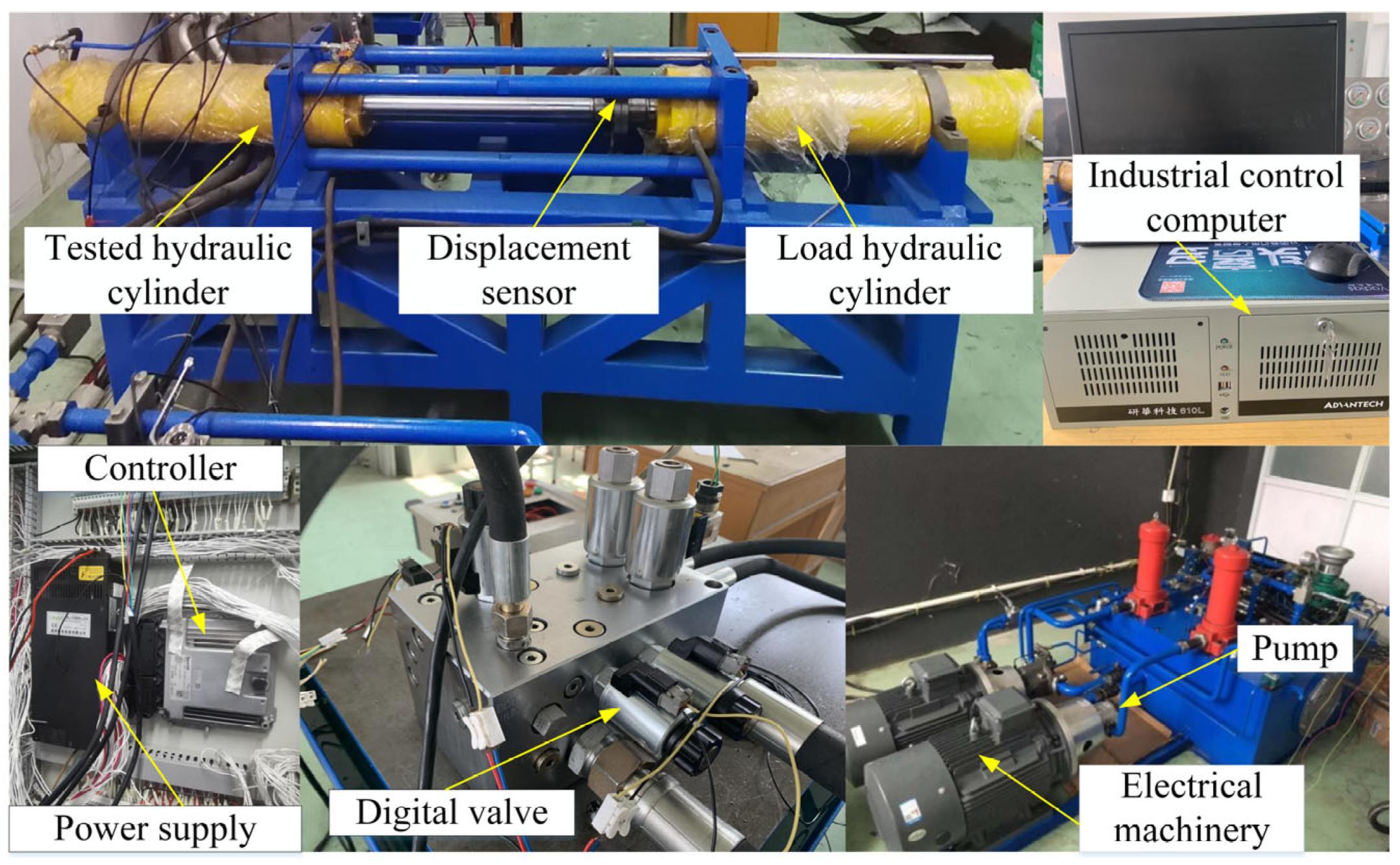
In order to further assess the effectiveness and applicability of the proposed control strategy, comparative experiments were carried out on a digital valve-controlled hydraulic cylinder test bench. Figure 14 illustrates the experimental platform, which was comprised mainly of a hydraulic system consisting of a position test system and a load simulation system. The digital valve in the position test system was WS22GD, whose control voltage signal was 12 V. The maximum stroke of the piston rod was 0.6 m, and the displacement of the piston rod was measured by the drawstring displacement transducer MPS-S-650 mm-MA from Shenzhen Miran Technology Co., Ltd. in Shenzhen, China, whose stroke was in the range of 0–0.35 m. The output signal was 4–20 mA, and the proportional relief valve was DBE10-30B/200YM. The motor was Y160L-4-B35, and the variable pump was HA10Vs045DFLR/31R-PPA12N00. The industrial computer was the standard industrial computer of Advantech Technology, and the motion controller was the RC28-14 from Rexroth.

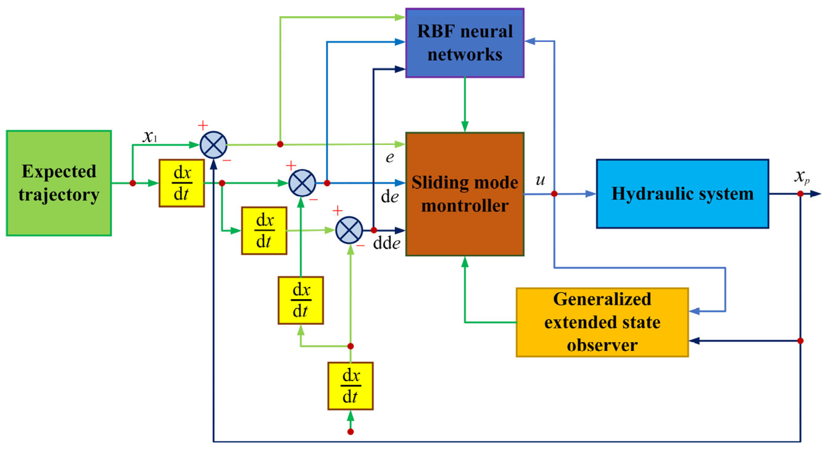
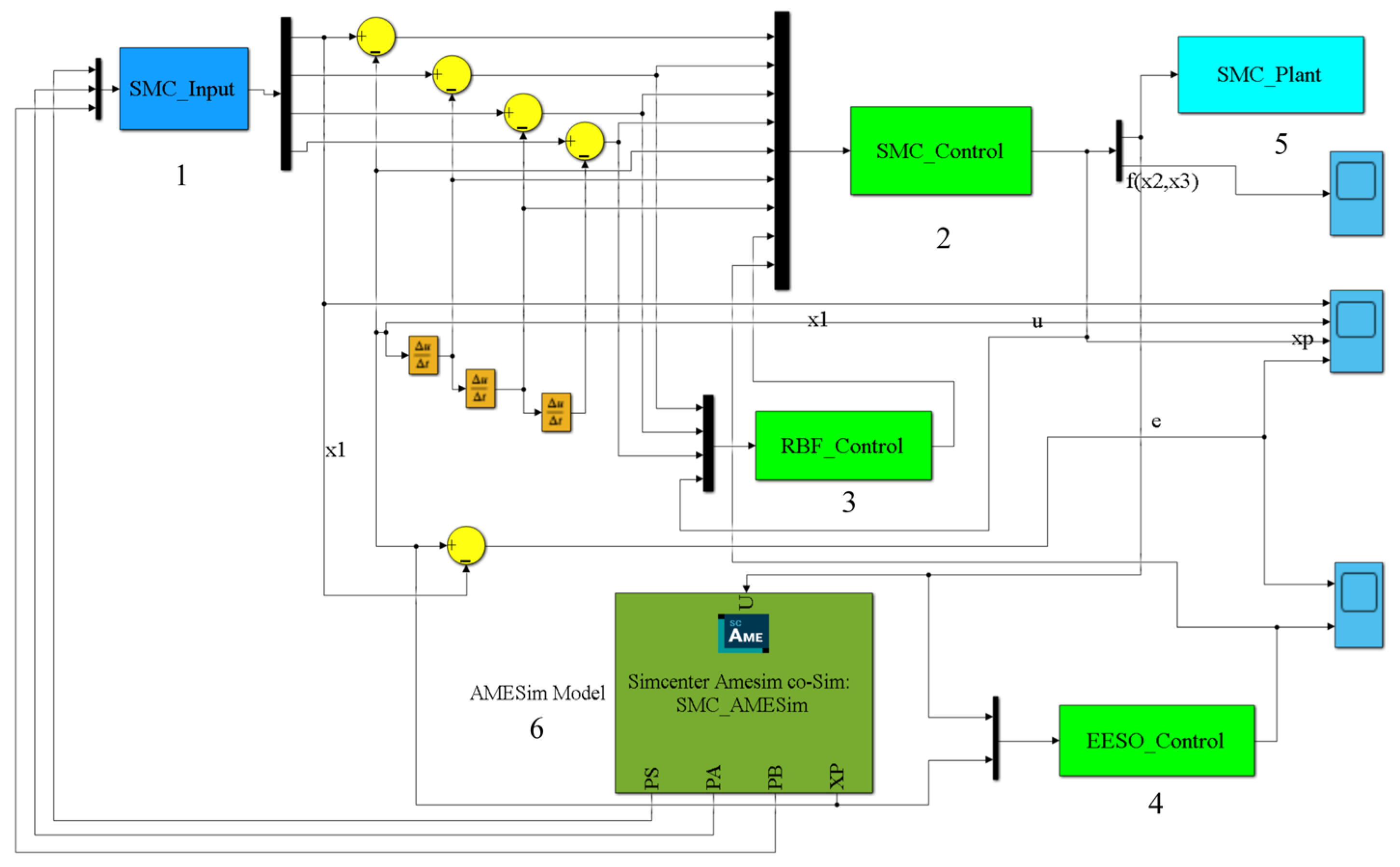
In this paper, the motion controller RC28-14 was utilized as the lower-level computer, and the industrial computer installed with MATLAB served as the upper-level computer. The control algorithm is depicted in Figure 3. Communication between Simulink and the RC28-14 controller was achieved through PeakCAN, with the communication mode being CAN communication. Simulink was used to send high-speed switching digital valve CAN messages to the RC28-14 controller to control the valve’s operation. The RC28-14 controller, in turn, emitted sensor CAN messages to Simulink to provide the necessary parameters for the control algorithm. The control sampling period lasted for 2 ms, enabling closed-loop tracking control of the actual loading displacement and the target loading displacement of the load hydraulic cylinder.

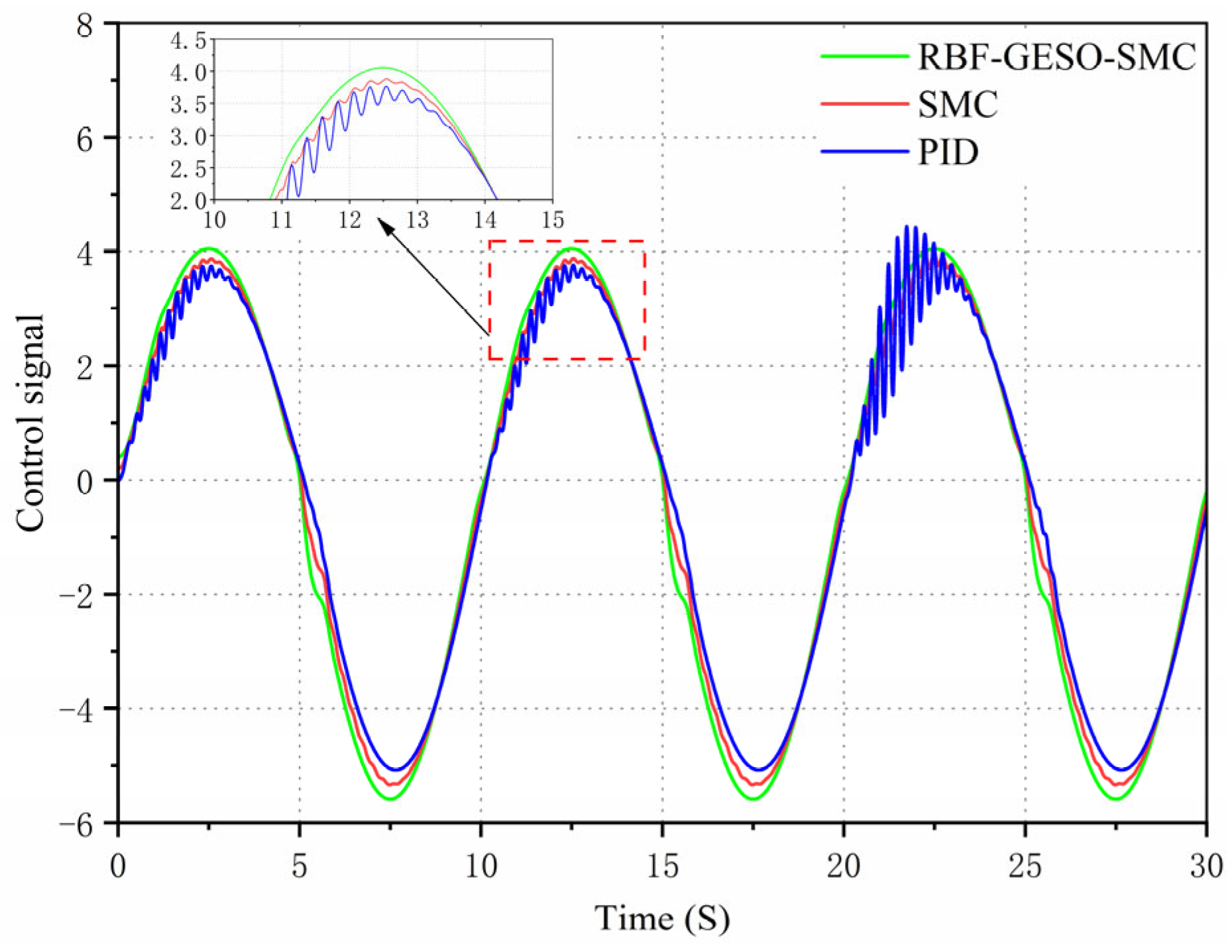
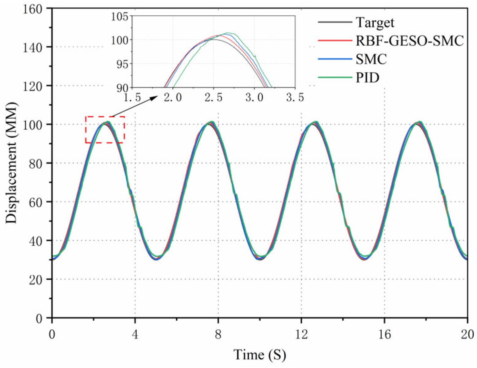
To ascertain the control effect of the RBF-GESO-SMC controller on the load hydraulic cylinder, two experiments were implemented to validate the software simulation results presented earlier. The control strategy proposed in this paper was compared with a traditional PID controller whose parameters were optimized using the Z-N method and an unoptimized SMC controller for verification purposes. The first experiment adopted a sinusoidal signal with an amplitude of 100 mm and a frequency of 0.2 Hz as the target signal, thereby verifying the tracking performance of the three control strategies for the target signal. The second experiment employed a ramp signal with a period of 20 s, a lower limit of 50 mm, and an upper limit of 120 mm as the target signal to verify the tracking performance and transient response characteristics of the three control strategies for the target signal.

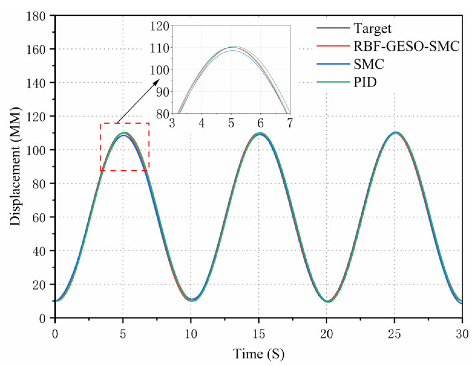
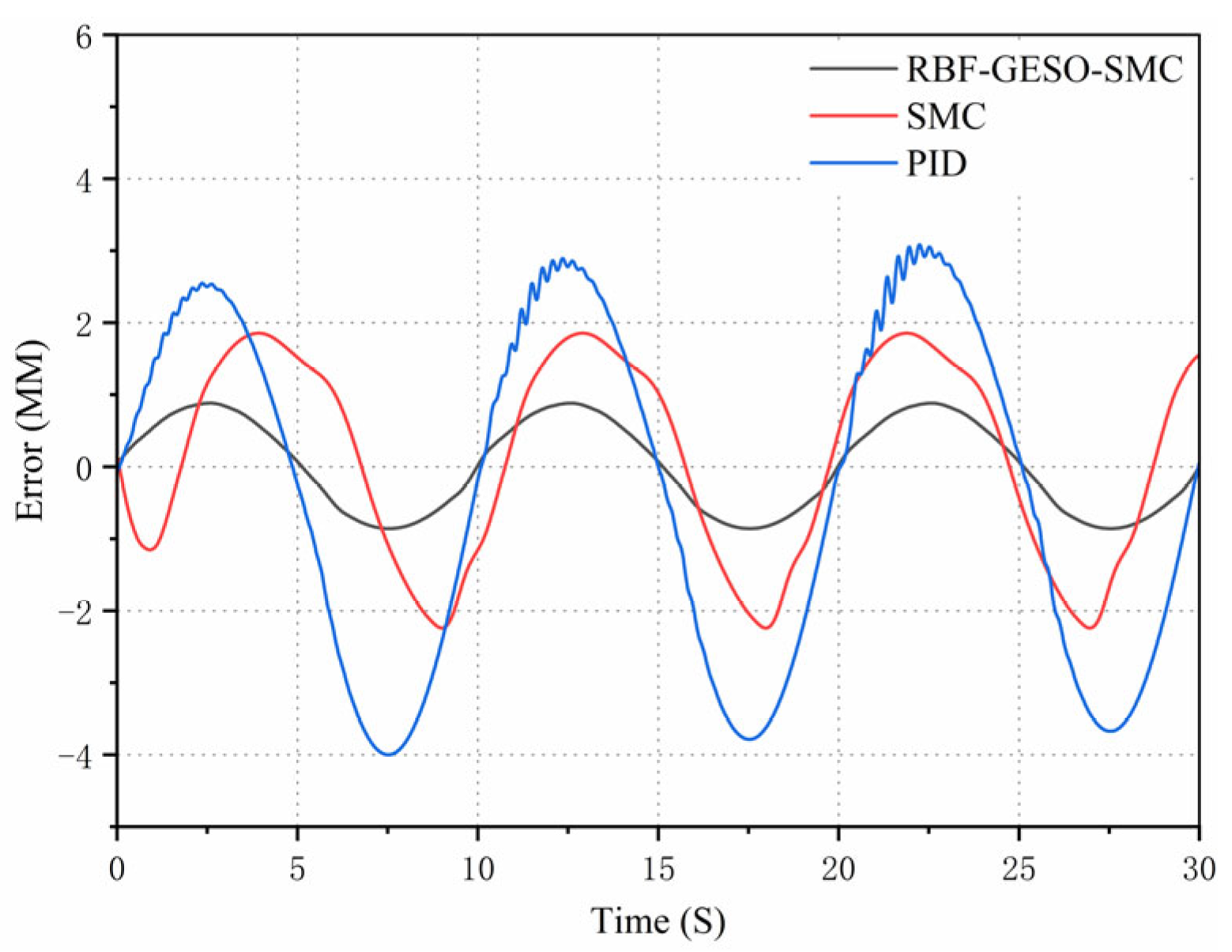
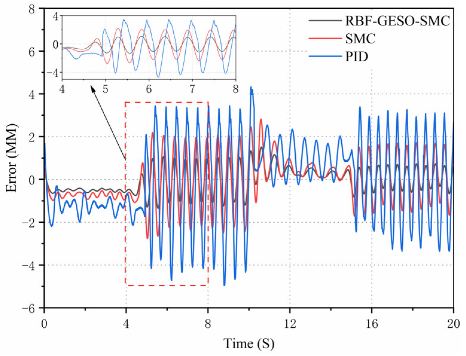
Firstly, to verify the displacement tracking performance of the RBF-GESO-SMC controller, the target signal was configured as a sinusoidal signal with an amplitude of 100 mm and a frequency of 0.2 HZ. The displacement response curves and error curves of the hydraulic cylinders under the three types of control are shown in Figure 15 and Figure 16.

As evident from the curves in Figure 15 and Figure 16, the tracking curve of the RBF-GESO-SMC controller closely aligned with the target curve, and the error amplitude of the peak-valley values was relatively small. Under the RBF-GESO-SMC controller, the maximum displacement tracking error was confined to be approximately 1.05 mm, with no discernible lead or lag in response. For the SMC controller, the maximum displacement tracking error was approximately 2.89 mm, and the lag phenomenon was quite obvious. Under the traditional PID controller, the maximum displacement tracking error was approximately 4.79 mm, accompanied by a conspicuous lag phenomenon. Compared with the SMC controller, the maximum displacement tracking error of the RBF-GESO-SMC controller was reduced by approximately 63.7%. Compared with the traditional PID controller, the maximum displacement tracking error of the RBF-GESO-SMC controller was diminished by approximately 78.1%. From the above analysis, it can be concluded that the RBF-GESO-SMC controller exhibited better performance in adapting to parameter uncertainties and nonlinear external disturbances. This enhanced the controller’s capabilities, effectively suppressing external disturbances.

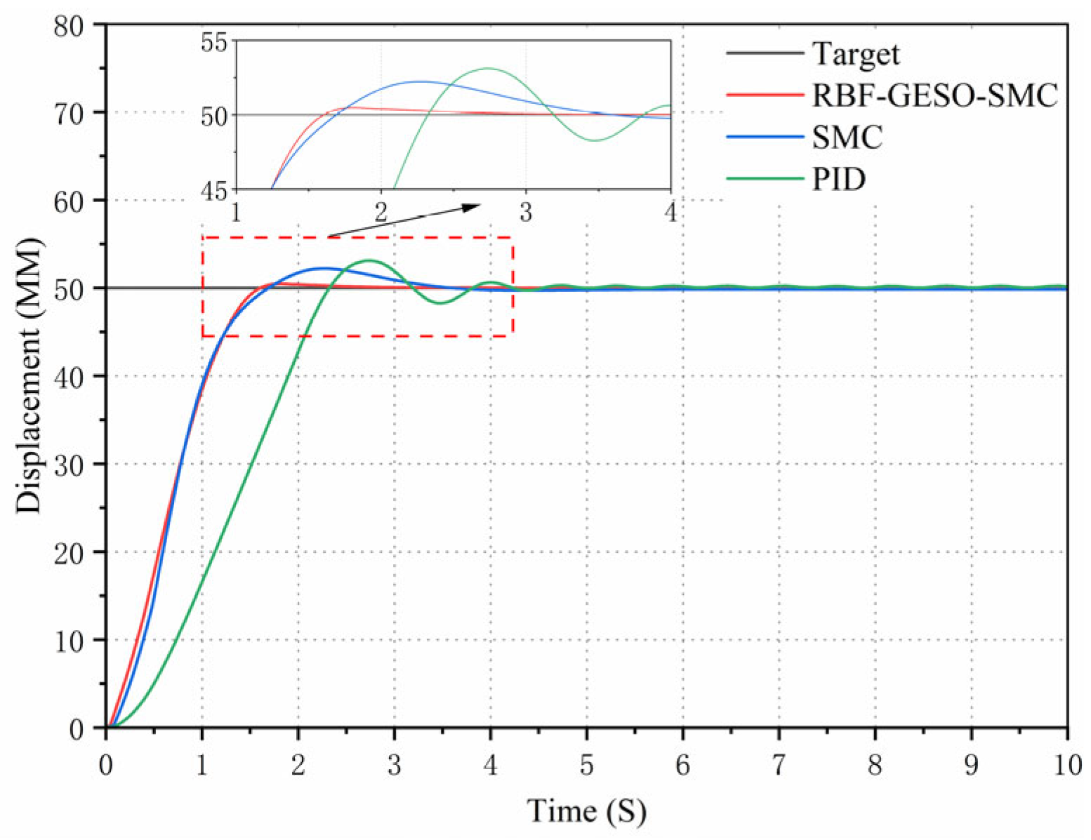
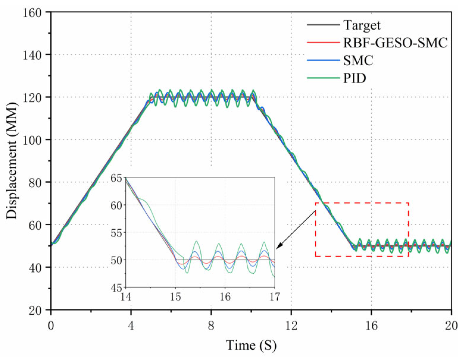
Finally, to validate the tracking performance of the RBF-GESO-SMC controller under external disturbances, a ramp signal with a period of 20 s and an amplitude ranging from 50 mm to 120 mm was employed as the target signal. The displacement response curves and error curves of the hydraulic cylinders under the three types of control are depicted in Figure 17 and Figure 18.

As can be seen from the curves in Figure 17 and Figure 18, the tracking curve of the RBF-GESO-SMC controller exhibited minimal susceptibility to external disturbances. Under the RBF-GESO-SMC controller, the disturbance tracking error was confined within 1.51 mm, and the response was rapid. For the SMC controller, the disturbance tracking error was 2.82 mm, and the response was relatively slow. Under the traditional PID controller, the disturbance tracking error was 4.95 mm, with a significantly lagged response. According to the experimental analysis, it can be inferred that the RBF-GESO-SMC controller possessed superior dynamic characteristics. That is, the system’s robustness to combined disturbances was enhanced, allowing for rapid and precise signal tracking, thus fulfilling the predefined tracking control objectives of the system.

The control performance indicators of the PID controller, SMC controller, and RBF-GESO-SMC controller in the experiment are detailed in

Table 4. Comparison of experimental control signal results.

Signal	Parameter	PID	SMC	RBF-GESO-SMC
Sinusoidal Signal	$\mathrm{Maximum} \mathrm{absolute} \mathrm{error} M_e$ (mm)	4.79	2.89	1.05
	$\mathrm{Average} \mathrm{value} {\mu }_e$ (mm)	2.56	1.15	0.51
	$\mathrm{Standard} \mathrm{deviation} {\sigma }_e$ (mm)	1.23	0.68	0.25
Ramp Signal	$\mathrm{Maximum} \mathrm{absolute} \mathrm{error} M_e$ (mm)	4.95	2.82	1.51
	$\mathrm{Average} \mathrm{value} {\mu }_e$ (mm)	1.62	0.94	0.48
	$\mathrm{Standard} \mathrm{deviation} {\sigma }_e$ (mm)	1.02	0.62	0.30

.

By comparing the performance indicators of the three controllers in Table 4, under the experimental sinusoidal signal, the RBF-GESO-SMC controller demonstrated notable performance enhancements, with the maximum tracking error, average tracking error, and standard deviation of the tracking error of the RBF-GESO-RBF controller reduced by 78.1%, 80.1%, and 79.7%, respectively, compared with the PID controller, and by 63.7%, 55.7%, and 63.2%, respectively, compared with the SMC controller. Similarly, under the experimental ramp signal, it can be found that the maximum tracking error, average tracking error, and standard deviation of the tracking error of the RBF-GESO-RBF controller were reduced by 69.5%, 70.9%, and 70.6%, respectively, compared with the PID controller, and by 46.5%, 48.9%, 51.6%, respectively, compared with the SMC controller. The findings reveal that the RBF-GESO-SMC controller outperformed the other two controllers in the output of the three target signals.

6. Conclusions

This article addresses issues such as jitter, unknown dead zone nonlinearity, and time variance in electro-hydraulic proportional systems in hydraulic cylinder position control. An independent metering control system with digital valves was employed to regulate the position control of the hydraulic cylinder within the hydraulic system, and a high-order sliding mode digital valve control strategy was incorporated based on an RBF neural network and generalized extended state observer. Among them, the introduction of the RBF neural network and generalized extended state observer aimed to mitigate the effects caused by uncertainty and external disturbances of digital valve control systems. The RBF neural network enabled the estimation and compensation for parameter uncertainty through online approximation of unknown matching parameters and correction of adaptive control laws. Additionally, the generalized extended state observer offered real-time observation of external disturbances and fed the observed values back to the controller for prompt disturbance compensation. Finally, the Lyapunov function was utilized to verify the stability of the proposed control strategy; however, practical implementation of this proposed technology may encounter some obstacles in actual engineering scenarios. Therefore, it is imperative to enhance the robustness of digital valve control models and adjustable models to navigate the uncertainty of actual systems and meet the rapid response requirements of practical engineering. Meanwhile, optimizing the parameter settings of the controlled system is crucial for minimizing computational complexity and enhancing real-time observation capabilities. Looking forward, these challenges are expected to be surmounted progressively, thereby promoting further advancement and broader application of related technologies.

Then, through MATLAB/Simulink simulation, under conditions of parameter uncertainties and unknown external disturbances within the system, the simulation results suggest that the proposed control strategy exhibited a higher expected trajectory tracking accuracy compared with the SMC controller and the traditional PID controller. Compared with the SMC controller, the response speed increased by 13.6%, and the displacement tracking control accuracy error decreased by 60.5%. In contrast to the traditional PID controller, the response speed increased by 34.5%, and the error in displacement tracking control accuracy was reduced by 78.0%. Based on the analysis of simulation data, the control strategy proposed in this paper outperformed both the SMC controller and the traditional PID controller in terms of tracking performance and transient response performance under different operating conditions. However, the simulation results were obtained by using theoretical values for many system parameters, which means they are somewhat idealistic. Therefore, it is still crucial to establish a digital valve-controlled hydraulic cylinder test bench for displacement loading testing to verify the practical feasibility of the control strategy proposed in this paper.

Finally, the control strategy proposed in this article was applied to the digital valve-controlled hydraulic cylinder system for displacement loading testing for experimental verification. The results of the step and sine experiments revealed that this control strategy significantly enhanced the tracking accuracy and anti-interference performance of the electro-hydraulic servo system. Compared with the SMC controller, the error in displacement tracking control accuracy was decreased by 63.7%. Compared with the traditional PID controller, the displacement tracking control accuracy error was decreased by 78.1%. According to the above experiment, this control method significantly improved the tracking accuracy and anti-interference robustness of the digital valve-controlled hydraulic cylinder system. Its tracking accuracy, transient response speed, and anti-interference ability can effectively meet the accuracy and transient response performance requirements in actual hydraulic cylinder operation.

References

1. Jia, R.; Zhang, J.; Ding, R.; Zhang, F.; Shen, J.; Xu, B. Active Damping Control of the Large-scale Flexible Hydraulic Manipulators with Independent Metering System. Int. J. Fluid Power 2024, 25, 163–182. [Google Scholar] [CrossRef]
2. Zhang, J.; Wang, D.; Ding, R.; Chen, Z.; Yang, C.; Xu, B.; Chen, M. A fault detection and isolation method for independent metering control system based on adaptive robust observer. Measurement 2025, 241, 115707. [Google Scholar] [CrossRef]
3. Yavuz Coskun, M.; Itik, M. Position control of a digital electrohydraulic system with limited sensory data using double deep q-network controller. Expert Syst. Appl. 2024, 252, 24275. [Google Scholar]
4. Cecchin, L.; Ohtsuka, T.; Trachte, A.; Diehtl, M. Model Predictive Controller for Hydraulic Cylinders with Independent Metering Control Valves. IFAC Pap. 2024, 58, 281–287. [Google Scholar] [CrossRef]
5. Milecki, A.; Ortman, J. Electrohydraulic linear actuator with two stepping motors controlled by overshoot-free algorithm. Mech. Syst. Signal Process. 2017, 96, 45–57. [Google Scholar] [CrossRef]
6. Chen, J.; Jiang, H.; Kong, X.; Ai, C. Mode switching control of independent metering fluid power systems. ISA Trans. 2025, 158, 735–748. [Google Scholar] [CrossRef]
7. Nguyen, T.H.; Do, T.C.; Phan, V.D.; Ahn, K.K. Working Performance Improvement of a Novel Independent Metering Valve System by Using a Neural Network-Fractional Order-Proportional-Integral-Derivative Controller. Mathematics 2023, 11, 4189. [Google Scholar] [CrossRef]
8. Yan, H.; Liu, Y.; Ma, L. Mechanism of Temperature’s Acting on Electro-Hydraulic Servo Valve. IEEE Access 2019, 7, 80465–80477. [Google Scholar] [CrossRef]
9. Yang, X.; Cui, Y.; Yuan, Z.; Hang, J. RISE-based adaptive control of electro-hydraulic servo system with uncertain compensation. Math. Biosci. Eng. 2023, 20, 9288–9304. [Google Scholar] [CrossRef]
10. De Matos Torre, N.M.; Bonamigo, A. Action research of lean 4.0 application to the maintenance of hydraulic systems in steel industry. J. Qual. Maint. Eng. 2024, 30, 341–366. [Google Scholar]
11. Yang, Z.; Hu, X.; Xu, F.; Wu, D.; Liu, Y. Large-range dynamic characteristic adjustment of high-speed on-off valve for water hydraulic manipulators based on multistage voltage and double sliding mode control. Measurement 2025, 242, 116094. [Google Scholar] [CrossRef]
12. Zhang, Q.; Kong, X.; Yu, B.; Ba, K.; Jin, Z.; Kang, Y. Review and Development Trend of Digital Hydraulic Technology. Appl. Sci. 2020, 10, 579. [Google Scholar] [CrossRef]
13. Meng, L.; Wu, D.; Gao, H.; Ye, X.; Liu, H.; Liu, Y. Multi-objective optimization of a wet electromagnet-driven water hydraulic high-speed on/off valve for underwater manipulator in deep sea. Measurement 2025, 239, 115443. [Google Scholar] [CrossRef]
14. Bruno, N.; Zhu, Y.; Liu, H.; Gao, Q.; Li, Y. Development of a piezoelectric high speed on/off valve and its application to pneumatic closed-loop position control system. J. Mech. Sci. Technol. 2019, 33, 2747–2759. [Google Scholar] [CrossRef]
15. Yang, G.; Jiang, P.; Lei, L.; Wu, Y.; Du, J.; Li, B. Adaptive Backstepping Control of Vacuum Servo System Using High-Speed on-off Valves. IEEE Access 2020, 8, 129799–129812. [Google Scholar] [CrossRef]
16. Xu, Y.X.; Zhu, S.Q. Dual Piezoelectric-Driving Pneumatic Digital Valve Control Method Simulation Research. Adv. Mater. Res. 2013, 816, 367–370. [Google Scholar] [CrossRef]
17. Qi, Z.; Xu, E.; Xie, G.; Wang, X.; Li, Y. Dynamic performance and temperature rising characteristic of a high-speed on/off valve based on pre-excitation control algorithm. Chin. J. Aeronaut. 2023, 36, 445–458. [Google Scholar]
18. He, W.; Chen, Z.; Huang, J.; Quan, L.; Zhao, B. Development of High-Speed On–Off Valves and Their Applications. Chin. J. Mech. Eng. 2022, 35, 67. [Google Scholar]
19. Qiu, H.; Qi, S. Simulation Research of Hydraulic Stepper Drive Technology Based on High Speed On/Off Valves and Miniature Plunger Cylinders. Micromachines 2021, 12, 438. [Google Scholar] [CrossRef]
20. Yao, J.; Wang, P.; Dong, Z.; Jiang, D.; Sha, T. A novel architecture of electro-hydrostatic actuator with digital distribution. Chin. J. Aeronaut. 2020, 34, 224–238. [Google Scholar] [CrossRef]
21. Liu, Z.-H.; Gao, Q.-H.; Deng, G.; Niu, H.-L.; Li, J.-Y. The position control of hydraulic cylinder based on high-speed on-off valve. Int. J. Model. Identif. Control 2014, 22, 54–67. [Google Scholar] [CrossRef]
22. Gao, Q.; Liu, H.; Lan, B.; Zhu, Y. A model-based sliding mode control with intelligent distribution for a proportional valve driven by digital valve arrays. ISA Trans. 2024, 151, 312–323. [Google Scholar] [CrossRef] [PubMed]
23. Kong, X.; Majmudar, H.; Zhang, W. A multi-switching mode intelligent hybrid control of electro-hydraulic proportional systems. Proc. Inst. Mech. Eng. Part C J. Mech. Eng. Sci. 2019, 233, 120–131. [Google Scholar] [CrossRef]
24. Lee, C.; Jeon, C.-W.; Han, X.; Kim, J.H.; Kim, H.-J. Application of Electrohydraulic Proportional Valve for Steering Improvement of an Autonomous Tractor. J. Biosyst. Eng. 2022, 47, 167–180. [Google Scholar] [CrossRef]
25. Thien, T.D.; Xuan, B.D.; Kyoung Kwan, A. Adaptive Backstepping Sliding Mode Control for Equilibrium Position Tracking of an Electrohydraulic Elastic Manipulator. IEEE Trans. Ind. Electron. 2020, 67, 3860–3869. [Google Scholar]
26. Hao, H.; Yan, H. The pressure control of independent load port electro-hydraulic load simulation system using fixed time integral sliding mode active disturbance rejection. Sci. Rep. 2024, 14, 29064. [Google Scholar] [CrossRef]
27. Sun, C.; Li, J.; Tan, Y.; Duan, Z. Proposed Feedback-Linearized Integral Sliding Mode Control for an Electro-Hydraulic Servo Material Testing Machine. Machines 2024, 12, 164. [Google Scholar] [CrossRef]
28. Liu, R.; Wang, Z.; Jia, P.; Yan, G.; Zhang, T.; Jia, C.; Chen, G. Research on Pressure Control of an Electro-Hydraulic Servo System Based on Sliding-Mode Variable-Structure Direct Torque Control. Processes 2022, 11, 92. [Google Scholar] [CrossRef]
29. Van Chuong, L.; Sy Phuong, H.; Dinh Tu, D.; Van Du, P.; Thai Son, D.; Van Nam, D. Adaptive Terminal Sliding Mode Control Using RBF Neural Network for Industrial Robot Manipulators. In Advances in Information and Communication Technology, Proceedings of the 3rd International Conference ICTA 2024, Thai Nguyen, Vietnam, 16–17 November 2024; Springer: Berlin/Heidelberg, Germany, 2025; pp. 591–598. [Google Scholar]
30. Yao, Z.; Yao, J.; Yao, F.; Xu, Q.; Xu, M.; Deng, W. Model reference adaptive tracking control for hydraulic servo systems with nonlinear neural-networks. ISA Trans. 2020, 100, 396–404. [Google Scholar] [CrossRef]
31. Jiang, S.; Hui, W.; Guochao, Z. Research on neural network model reference adaptive disturbance rejection control of digital hydraulic cylinder. Adv. Mech. Eng. 2022, 14. [Google Scholar] [CrossRef]
32. Fang, Q. Estimation of Navigation Mark Floating Based on Fractional-Order Gradient Descent with Momentum for RBF Neural Network. Math. Probl. Eng. 2021, 2021, 6681651. [Google Scholar] [CrossRef]
33. Yun, C.-G.; Sin, Y.-C.; Ri, H.-R.; Jo, K.-N. Trajectory tracking control of a three-wheeled omnidirectional mobile robot using disturbance estimation compensator by RBF neural network. J. Braz. Soc. Mech. Sci. Eng. 2023, 45, 432. [Google Scholar] [CrossRef]
34. Sharafati, A.; Tafarojnoruz, A.; Shourian, M.; Yaseen, Z.M. Simulation of the depth scouring downstream sluice gate: The validation of newly developed data-intelligent models. J. Hydro-Environ. Res. 2019, 29, 20–30. [Google Scholar] [CrossRef]
35. Sharafati, A.; Tafarojnoruz, A.; Motta, D.; Yaseen, Z.M. Application of nature-inspired optimization algorithms to ANFIS model to predict wave-induced scour depth around pipelines. J. Hydroinform. 2020, 22, 1425–1451. [Google Scholar] [CrossRef]
36. Xiong, J.; Liu, S.; Zhang, H. Design and validation of ADRC-based variable thrust control for a low-cost ethanol-oxygen rocket engine. Control. Eng. Pract. 2025, 156, 106200. [Google Scholar] [CrossRef]
37. Zhuang, X.; Tian, Y.; Wang, H.; Sofiane, A.-A. Event-triggered joint adaptive high-gain observer design for delayed output-sampled nonlinear systems with unknown parameters and output injection. Commun. Nonlinear Sci. Numer. Simul. 2025, 142, 108541. [Google Scholar] [CrossRef]
38. Ling, Z.; Qi, L.; Liu, B.; Cheng, H. Trajectory Tracking Control of a One Degree of Freedom Manipulator Based on a Switched Sliding Mode Controller With a Novel Extended State Observer Framework. IEEE Trans. Syst. Man Cybern. Syst. 2019, 49, 1110–1118. [Google Scholar]
39. Li, Y.; Li, A.; Pang, K.; Zhang, Z.; Song, G. Fault-tolerant control of nonlinear quadrotor formation based on linear extended state observer and estimated minimum learning parameter. Aerosp. Sci. Technol. 2025, 158, 109909. [Google Scholar] [CrossRef]
40. Sui, B.; Zhang, J.; Liu, Z. Extended state observer based prescribed-time trajectory tracking control for USV with prescribed performance constraints and input saturation. Ocean. Eng. 2025, 316, 120005. [Google Scholar] [CrossRef]
41. Yang, T.; Zhang, B.; Hong, H.; Chen, Y.; Yang, H.; Tongman, W. Motion control for earth excavation robot based on force pre-load and cross-coupling compensation. Autom. Constr. 2022, 141, 104402. [Google Scholar] [CrossRef]
42. Liu, Z.H.; Gao, Q.H.; Niu, H.L. The Position Control of the Hydraulic Cylinder Controlled by the High-Speed On-off Valve. Sens. Transduc. 2013, 160, 590–601. [Google Scholar]
Figure 1. Digital valve-controlled hydraulic cylinder position control schematic.
Actuators 14 00221 g001
Figure 2. Schematic diagram of oil flow direction under various operating conditions.
Actuators 14 00221 g002
Figure 3. Schematic diagram of sliding mode control of hydraulic cylinder using RBF neural network and generalized extended state observer.
Actuators 14 00221 g003
Figure 4. Schematic diagram of RBF neural network structure.
Actuators 14 00221 g004
Figure 5. Simulink simulation model. 1—Expected trajectory and feedback input; 2—sliding mode controller; 3—RBF neural network; 4—generalized extended state observer; 5—theoretical model of hydraulic system; 6—co-simulation interface.
Actuators 14 00221 g005
Figure 6. Simulation model of the hydraulic system. 1—Hydraulic station; 2—system fuel supply pressure sensor; 3—co-simulation interface; 4—signal conversion module; 5—gain; 6~9—digital valve; 10—gain; 11—A chamber pressure sensor; 12—B chamber pressure sensor; 13—hydraulic cylinder; 14—displacement sensor; 15—disturbance form; 16—disturbing signal.
Actuators 14 00221 g006
Figure 7. Generalized extended state observer for estimating external disturbances.
Actuators 14 00221 g007
Figure 8. RBF neural network fitting uncertain terms.
Actuators 14 00221 g008
Figure 9. Step signal simulation response curve.
Actuators 14 00221 g009
Figure 10. Step signal simulation error curve.
Actuators 14 00221 g010
Figure 11. Sinusoidal signal simulation response curve.
Actuators 14 00221 g011
Figure 12. Sinusoidal signal simulation error curve.
Actuators 14 00221 g012
Figure 13. Control strategy signal output curve.
Actuators 14 00221 g013
Figure 14. The control platform of the hydraulic system.
Actuators 14 00221 g014
Figure 15. Sinusoidal signal response curve.
Actuators 14 00221 g015
Figure 16. Sinusoidal signal error curve.
Actuators 14 00221 g016
Figure 17. Ramp signal response curve.
Actuators 14 00221 g017
Figure 18. Ramp signal error curve.
Actuators 14 00221 g018