Efficient CoM Motion Planning for Quadruped Robots’ Quasi-Static Walking

Abstract

With the popularity of quadruped robots, the main challenge they must overcome is traversing unstructured environments. Current methods that allow modern robots to traverse challenging terrain are unsuitable for situations at the edge of robot performance, where torque limits and contact forces must be carefully considered. This paper will investigate a way of generating feasible center of mass (CoM) trajectories applicable in such cases. A feasible CoM trajectory is one that the robot can perform considering contact, torque, and reachability constraints. We improve the existing method for finding feasible CoM regions, yielding a thirty times speedup so that it can run under 1 ms. Based on that improvement, we introduce a new iterative CoM planner that sequentially solves prioritized constrained IK and computes feasible regions. That way, we guarantee the satisfaction of contact constraints, torque constraints, and reachability. The planned motion was performed using a whole-body controller. We tested the approach on high-fidelity simulation and on real Solo12 quadruped, achieving the control loop frequency of 1 kHz. The whole codebase has been disclosed on GitHub.

1. Introduction

Based on the means of locomotion, mobile robots can be classified into three categories: legged robots, wheeled robots, and tracked robots [1]. The locomotion system is an essential design characteristic and depends on the intended use of the robot due to the significant differences in maneuverability, controllability, efficiency, and stability. There are different subtypes of locomotion systems, each with advantages and disadvantages that have been explored in the past [2]. The main advantage of legged robots lies in the potential to traverse a lot of different terrains, similar to a human or an animal. There are many types of legged robots based on the number of legs. The most important include biped (humanoid) robots, quadruped (four-legged) robots, and hexapod (six-legged) robots. Quadruped robots present the best choice among legged robots in terms of mobility and stability of locomotion, as the robot’s four legs are easily controlled, designed, and maintained compared to two or six legs.

Recently, quadrupeds started becoming ubiquitous as several different robotics platforms like Boston Dynamics’ Spot and Unitree’s Go2 became available in the market, with the latter costing no more than a few thousand dollars. ANYbotics, a spin-off from ETH Zuerich, started providing end-to-end industrial inspection services using their in-house developed quadruped ANYmal [3].

The prime challenge all mentioned robots must overcome is traversing unstructured environments. Two distinct approaches arose, those based on model predictive control [4,5] and those based on reinforcement learning [6,7], and even some hybrid ones combining both approaches [8]. These approaches could accommodate swift and dynamic motions on different types of terrain. Although terrain and obstacles were challenging, these methods do not apply to cases at the edge of the robot’s performance, where torque constraints and contact forces must be carefully considered. The need to move in a challenging terrain has been recognized by the robotics society, resulting in a Quadruped Robotics Challenge (QRC) [9]. In that challenge, the robot is supposed to scale different types of obstacles including steps, sloped rails and steps. That is why planning feasible trajectories becomes essential to the robot control system. A feasible trajectory is one that ensures contact stability while respecting joint torque and kinematic limits. This paper will consider a way of generating feasible CoM trajectories that are applicable when moving across very challenging terrain.

2. Related Works

More than half a century ago, Vukobratovć introduced the first indicator of dynamic balance called Zero Moment Point (ZMP) [10]. It stated that the walking mechanism is dynamically balanced if a point within the support polygon (excluding its edge) exists, such that the total moment acting at that point in the horizontal plane equals zero, hence the name Zero Moment Point [11,12]. This notion assumed that the robot was walking on a flat surface and that friction was sufficiently large.

Initially, the hardware was the limitation for walking robots, but as hardware started catching up, it was evident that this indicator was insufficient. As a result, attempts to generalize the ZMP notion started to appear. In [13], Harada et al. studied the case with multiple contacts where the robot was touching the wall with its hands. The authors computed a polyhedron containing all contact points and conducted a geometric study to see if a robot could rotate around the edge of a polyhedron. Also, Generalized ZMP (GZMP) was introduced as a point on the ground surface for which the total moment in a horizontal plane from all contact forces equals zero. The robot is dynamically balanced if GZMP is within the support area obtained by the polyhedron projection on the ground surface. In a study that came out the same year, Hirukawa et al. [14] developed a criterion for multi-contact motion feasibility with arbitrary contact placement. The number and placement of contacts define a set of feasible wrenches applied to the system’s center of mass (CoM). It turned out that wrenches must be within the convex cone, and the motion is feasible if the sum of gravity and inertial forces is within that cone (gravity-inertial wrench cone (GIWC)). Although an improvement to ZMP, these criteria still assumed sufficient friction (implicitly assuming an infinite friction coefficient), and their applicability was showcased in only a few elementary cases, such as a robot walking up the stairs while holding a handrail or a robot leaning against the wall.

S. Caron et al. in [15] considered limited friction by approximating friction cones with a four-sided pyramid and assuming a rectangular shape of the contact patch, closely resembling the contact of a humanoid’s foot and the ground. Under such assumptions, they could derive closed-form formulae for the stability of planar contact with Coulomb friction. In [16], authors have found a general procedure for computing planar contact stability criteria for the arbitrary shape of the foot and arbitrary approximation of the friction cone. It shows that the contact wrench acting on the foot normalized by normal force is within a 5D convex polygon. Hence, constraint computation is reduced to calculating a convex hull of points in 5D. The same paper shows how tangential forces, vertical torque, and friction cone approximation influence the effective shape of the foot. The big tangential forces, normal torque, and coarse approximation lead to a smaller size of the effective area of the foot.

In [17], the authors have described how to compute GIWC using the double descriptor method [18]. That was the first time a technique addressed a general case with multiple arbitrarily spatially distributed contacts with limited friction. It is reported that computation of the gravito-inertial wrench cone for the case of a robot standing with both feet on the ground and four-sided friction pyramids as an approximation of the friction cone takes around 5 ms. Although significant progress has been made, the procedure is NP-complete, potentially slowing computation times for more complex cases. The same authors have used computed GIWC to derive an entire support area containing all ZMPs generated by valid contact forces [19]. After that, using the linear pendulum model LPM, the authors synthesized a walking controller, which was tested in simulation on an HRP-4 humanoid robot.

To overcome the NP-completeness of the double descriptor method, a polynomial time method for GIWC computation was developed in [20]. It describes reducing the spatially distributed contact to the planar case described in [16]. The GIWC is computed from a convex hull of points in 5D space, which has polynomial time complexity [21]. It reports the time of 1.6 ms for the robot standing with both feet on the ground and four-sided friction pyramids. It also considers more complex cases with three planar contacts with the environment (two feet and a hand) with eight-sided friction pyramids taking around 8 ms, proving that there is no explosion in computation time as the problem becomes complex. In [22], the same authors have described several typical cases with ground support surfaces for such cases. Authors have shown that in the case of multiple non-coplanar contacts, ZMP might go out of the convex hull of projected contact points while the system is still dynamically balanced.

The methods described until now are only considered if the nature of contact allows a specific motion. Actuation constraints were not considered at all, reducing the applicability of methods to real-life robots. One of the first methods considering actuation constraints was [23]. The authors have computed a convex Feasible Wrench Polytope (FWP), considering both actuation and contact constraints. They do so by first intersecting friction cones and force polytopes (a set of forces that actuators can produce at a contact point) for each contact, obtaining a bounded friction cone. Then, FWP is computed as a Minkowski sum of all bounded friction cones. The method produced a 6D convex polytope, which was hard to comprehend and use for planning; hence, in subsequent publications, the same authors have looked into a way to project it in a 2D plane, limiting themselves to quasi-static locomotion [24]. In that paper, the authors have modified the Iterative Projection method first introduced in [25] to define feasible region, an actuation-aware extension of the support region. The IP, in essence, is an efficient way of finding the intersection of a 6D polytope with a 2D plane. The further improvement of a method is given in [26]. The technique has been extended to cases where the external force (apart from gravity) is acting on the robot, the intersection plane is not necessarily horizontal as in [24], and most importantly, motion feasibility from the IK perspective is considered for the first time. That new indicator is used to plan quasi-static CoM motion.

Although the final improvement is potent, it still suffers from several issues. The feasible region is just a local approximation, as it depends on the joint configuration for computing the Jacobian. Also, its computation is relatively slow (reported to be around 18 ms in [26]) for having some sequential refinement of the feasible region or having the ability to perform multiple computations during a single planning step. Ultimately, because of that, no guaranteed planned motion is possible. The feasible region is approximated around the starting point but never recomputed for the final CoM position. That led to the introduction of big margins when motion is planned.

The contribution of this research is twofold:

• We introduce the Recursively Expanding Iterative Projection (IP) method that outperforms previous methods, described in Section 3.1, by 15 times and allows us to compute feasible regions in less than 1 ms.
• Leveraging an increase in computation efficiency, we introduce a new iterative CoM planner that solves iteratively inverse kinematics (IK) and computes feasible regions. In this way, we ensure the robot can reach its destination and maintain static equilibrium.

3. Improving Feasible Region Computation

Before describing the improvements, let us revisit the actuation-aware IP algorithm from [24]. That is the method we are trying to improve.

3.1. IP Revisited

The region is generated by the algorithm described in Algorithm 1. It starts from two coarse approximations of the projected region: the inner approximation, which is always smaller than the projection, and the outer approximation, which is bigger than the projection. The algorithm iteratively expands the inner approximation in a direction ${\mathbf{a}}_i$ while shrinking the outer approximation in the opposite direction, as illustrated in Figure 1. In each iteration, the linear program (LP) is solved, finding a new extremal ${\mathbf{c}}_{xy}^{*}$ point along ${\mathbf{a}}_i$; this is added to the inner approximation while an edge with normal ${\mathbf{a}}_i$ passing through ${\mathbf{c}}_{xy}^{*}$ is added to the outer approximation [24].

The algorithm ensures the static stability of the robot via equality constraint (III.a), which states that the total wrench (denoted by $\mathbf{u}$) computed for point ${\mathbf{c}}_{xy}$ in the horizontal plane has total force equal to gravity and total torque equal to 0. Note that this program is independent of the position of the reference point in the vertical direction $c_z$. Matrix ${\mathbf{A}}_1\in {\mathbb{R}}^{6\times 3n_c}$ is a grasp matrix of all $n_c$ contacts, mapping the contact forces to the wrench at the reference point. ${\mathbf{A}}_2$ computes the angular component of the gravity wrench. The values of these matrices are:

$$\begin{gathered} \begin{array}{cc}\hfill {\mathbf{A}}_1& =\left[\left[\begin{array}{c}{\mathbf{I}}_{3\times 3}\\ {\left[{\mathbf{p}}_1\right]}_{\times }\end{array}\right],\cdots ,\left[\begin{array}{c}{\mathbf{I}}_{3\times 3}\\ {\left[{\mathbf{p}}_{n_c}\right]}_{\times }\end{array}\right]\right]\hfill \end{array} \\ \begin{array}{cc}\hfill {\mathbf{A}}_2& ={\left[\begin{array}{cccccc}0& 0& 0& 0& -mg& 0\\ 0& 0& 0& mg& 0& 0\end{array}\right]}^T\hfill \\ \hfill \mathbf{u}& ={\left[\begin{array}{cccccc}0& 0& 0& 0& 0& -mg\end{array}\right]}^T,\hfill \end{array} \end{gathered}$$

(1)

where ${\mathbf{p}}_i$ is position of contact i in world frame, m is the total mass of the robot and g is gravitational acceleration. Vector $\mathbf{f}\in {\mathbb{R}}^{3n_c}$ is a vector of all vertically stacked contact forces ${\mathbf{f}}_i$.

Inequality constraint III.b ensures that all contacts are stable by enforcing that all contact forces are within their respective friction cones. The contact constraint matrix is $\mathbf{B}\in {\mathbb{R}}^{n_s{n}_c\times 3n_c}$ is a block diagonal matrix where each block represents a friction cone for each contact given in span form ${\mathbf{S}}_{\mu }\in {\mathbb{R}}^{n_s\times 3}$:

$$\begin{array}{cc}\hfill \mathbf{B}& =\mathrm{diag}\left({\mathbf{B}}_1,{\mathbf{B}}_2,\cdots ,{\mathbf{B}}_{n_c}\right)\hfill \\ \hfill {\mathbf{B}}_i& =\left[\begin{array}{c}-{\mathbf{S}}_{\mu }{\mathbf{R}}_i^T\end{array}\right].\hfill \end{array}$$

(2)

${\mathbf{R}}_i$ is a rotation matrix representing the surface orientation of i-th contact. Each row of ${\mathbf{S}}_{\mu }$ is [16]:

$${\mathbf{S}}_{\mu k}=\left[\begin{array}{ccc}sin{\displaystyle \frac{2k\pi }{m}}& -cos{\displaystyle \frac{2k\pi }{m}}& \mu \end{array}\right];k=0\dots n_s-1,$$

(3)

where $n_s$ is the number of sides in a friction cone.

Algorithm 1 Feasible region IP algorithm.

Inputs: ${\mathbf{c}}_{xy},{\mathbf{p}}_1,\cdots ,{\mathbf{p}}_{n_c},{\mathbf{S}}_1^{\mu },\cdots ,{\mathbf{S}}_{n_c}^{\mu },{\underline{\mathit{\tau }}}_1\cdots {\underline{\mathit{\tau }}}_{n_j},{\overline{\mathit{\tau }}}_1\cdots {\overline{\mathit{\tau }}}_{n_j},$ Result: Local feasible region ${\mathcal{Y}}_{fa}$ Initialization: ${\mathcal{Y}}_{outer}$ and ${\mathcal{Y}}_{inner}$ while  $area\left({\mathcal{Y}}_{outer}\right)-area\left({\mathcal{Y}}_{inner}\right)>ϵ$  do     (I) Compute edges of ${\mathcal{Y}}_{inner}$     (II) Pick ${\mathbf{a}}_i$ based on the edge cutting off the largest fraction of ${\mathcal{Y}}_{outer}$     (III) Solve the linear problem:           ${\mathbf{c}}_{xy}^{*}=\mathrm{argmax}{\mathbf{a}}_i^T{\mathbf{c}}_{xy}$           such that:                 (III.a) ${\mathbf{A}}_1\mathbf{f}+{\mathbf{A}}_2{\mathbf{c}}_{xy}=\mathbf{u}$                 (III.b) $\mathbf{B}\mathbf{f}\le 0$                 (III.c) $\mathbf{G}\mathbf{f}\le \mathbf{d}$     (IV) Update the outer approximation ${\mathcal{Y}}_{outer}$     (V) Update the inner approximation ${\mathcal{Y}}_{inner}$ end while

Finally, inequality constraint III.c ensures that torque constraints in all joints are fulfilled, where upper and lower bounds on torque in joint i are denoted as ${\underline{\mathit{\tau }}}_i$ and ${\overline{\mathit{\tau }}}_i$, respectively. For quadruped robots, there is a 1-to-1 mapping between joint torques in the leg and contact forces if that leg is in contact with the environment. The assumption is that the leg is in a non-singular configuration and that the legs are 3DoF, which is a property of most, if not all, quadrupeds. Due to joint limits, most of them cannot find themselves in a singular configuration. The mapping is through a transpose Jacobian of the contact ${\mathbf{J}}_i$ and gravitational load on the leg ${\mathbf{g}}_i$ coming from the general model of multi-body system dynamics:

$${\mathit{\tau }}_{Li}+{\mathbf{J}}_i^T{\mathbf{f}}_{\mathbf{i}}={\mathbf{g}}_i,$$

(4)

where ${\mathit{\tau }}_{Li}$ represents the vector of torques in the leg forming i-th contact. Hence, matrix $\mathbf{G}\in {\mathbf{R}}^{6n_c\times 3n_c}$ and vector $\mathbf{d}$ assume forms:

$$\begin{array}{cc}\hfill \mathbf{G}& =\mathrm{diag}\left(\left[\begin{array}{c}{\mathbf{J}}_1^T\\ -{\mathbf{J}}_1^T\end{array}\right],\cdots ,\left[\begin{array}{c}{\mathbf{J}}_{n_c}^T\\ -{\mathbf{J}}_{n_c}^T\end{array}\right]\right)\hfill \end{array}$$

(5)

$$\begin{array}{cc}\hfill \mathbf{d}& =\left[\begin{array}{c}{\mathbf{g}}_1-{\underline{\mathit{\tau }}}_{L1}\\ -{\mathbf{g}}_1+{\overline{\mathit{\tau }}}_{L1}\\ ⋮\\ {\mathbf{g}}_{n_c}-{\underline{\mathit{\tau }}}_{L{n}_c}\\ -{\mathbf{g}}_{n_c}+{\overline{\mathit{\tau }}}_{L{n}_c}\end{array}\right]\hfill \end{array}$$

(6)

It is important to point out the slight difference between the presented algorithm and the original one described in [24]:

• Only point contacts are considered here, where the original can also accommodate surface contacts.
• Unlike the original version, where the number of sides in the friction pyramid is 4, there is no such assumption in the presented version.

These slight changes to the original algorithm do not influence its general applicability to quadruped robots.

3.2. Recursively Expanding IP

Since the friction cones are approximated with friction pyramids and joint torques have box constraints, the Feasible Contact Wrench is a convex polytope in 6D [23,24]. As a result, its projection to a 2D plane will be a convex polygon. The implication is that the solutions of LPs in Algorithm 1 are exactly the corners of the convex polygon of the feasible area. So, if we run the LP a sufficient number of times, we will perfectly reconstruct the feasible area ${\mathcal{Y}}_{fa}$, and ${\mathcal{Y}}_{fa}={\mathcal{Y}}_{outer}={\mathcal{Y}}_{inner}$ will be all equal. For this reason, we decided to remove the outer approximation altogether.

The recursive expanding IP algorithm is shown in Algorithm 2 and illustrated in Figure 2. Firstly, min and max points of the feasible region in some direction, e.g., x, are computed (steps I and II from Algorithm 2). After that, we recursively expand the surface by solving the previously noted LP starting from the midpoint of the already existing edge of the approximation ${\mathcal{Y}}_{fa}$, going in a direction normal to the edge (method ExpandFromLine). Once LP is solved and the new ${\mathbf{c}}_{xyi}^{*}$ is found, the point will be added to ${\mathcal{Y}}_{fa}$ if its distance from the starting edge is more than ${ϵ}_d$, and recursion will resume by expanding from two new edges of approximation ${\mathcal{Y}}_{fa}$. The LP would be solved exactly $2n_e$ times, where $n_e$ is the number of edges of the resulting feasible area.

Assuming we are using an optimization problem solver with warm starting to solve LPs, warm starting optimization from the mid-point of two known solutions yields significant speedup for two reasons:

• The solver will start from a feasible point, thus removing the need for computing the initial guess
• The optimization problem starts close to the solution, significantly reducing the number of iterations during optimization, thus reducing computation time.

Algorithm 2 Feasible region by recursive expansion IP algorithm.

Inputs: ${\mathbf{c}}_{xy},{\mathbf{p}}_1,\cdots ,{\mathbf{p}}_{n_c},{\mathbf{S}}_1^{\mu },\cdots ,{\mathbf{S}}_{n_c}^{\mu },{\underline{\mathit{\tau }}}_1\cdots {\underline{\mathit{\tau }}}_{n_j},{\overline{\mathit{\tau }}}_1\cdots {\overline{\mathit{\tau }}}_{n_j},$ Result: Local feasible region ${\mathcal{Y}}_{fa}$ function SolveLP($\mathbf{a}$, $\mathbf{p}$, $\mathbf{f}$)       Starting from $\mathbf{p}$ and $\mathbf{f}$ solve linear problem:        ${\mathbf{p}}^{*},{\mathbf{f}}^{*}=\mathrm{argmax}{\mathbf{a}}^T\mathbf{p}$        such that: ${\mathbf{A}}_1\mathbf{f}+{\mathbf{A}}_2\mathbf{p}=\mathbf{u}$             $\mathbf{B}\mathbf{f}\le 0$             $\mathbf{G}\mathbf{f}\le \mathbf{d}$ return ${\mathbf{p}}^{*}$, ${\mathbf{f}}^{*}$ end function procedure ExpandFromLine(${\mathbf{p}}_0$, ${\mathbf{f}}_0$, ${\mathbf{p}}_1$, ${\mathbf{f}}_1$, ${\mathcal{Y}}_{fa}$)       ${\mathbf{p}}_{mid}\leftarrow 0.5\left({\mathbf{p}}_0+{\mathbf{p}}_1\right);{\mathbf{f}}_{mid}\leftarrow 0.5\left({\mathbf{f}}_0+{\mathbf{f}}_1\right)$       Find $\mathbf{a}$ as a unit normal to vector ${\mathbf{p}}_1-{\mathbf{p}}_2$       ${\mathbf{p}}^{*}$, ${\mathbf{f}}^{*}\leftarrow \mathrm{SolveLP}\left(\mathbf{a},{\mathbf{p}}_{mid},{\mathbf{f}}_{mid}\right)$       if ${\mathbf{a}}^T\left({\mathbf{p}}^{*}-{\mathbf{p}}_{mid}\right)\ge {ϵ}_d$ then          ExpandFromLine(${\mathbf{p}}_0$, ${\mathbf{f}}_0$, ${\mathbf{p}}_{mid}$, ${\mathbf{f}}_{mid}$, ${\mathcal{Y}}_{fa}$)          ExpandFromLine(${\mathbf{p}}_{mid}$, ${\mathbf{f}}_{mid}$, ${\mathbf{p}}_1$, ${\mathbf{f}}_1$, ${\mathcal{Y}}_{fa}$)       else          Append ${\mathbf{p}}_0$ to ${\mathcal{Y}}_{fa}$       end if end procedure Initialize ${\mathcal{Y}}_{fa}$ to empty set (I) ${\mathbf{p}}_{left}$, ${\mathbf{f}}_{left}\leftarrow \mathrm{SolveLP}\left({\left[10\right]}^T,\mathbf{0},\mathbf{0}\right)$ (II) ${\mathbf{p}}_{right}$, ${\mathbf{f}}_{right}\leftarrow \mathrm{SolveLP}\left({\left[-10\right]}^T,{\mathbf{p}}_{left},{\mathbf{f}}_{left}\right)$ (III) ExpandFromLine(${\mathbf{p}}_{left}$, ${\mathbf{f}}_{left}$, ${\mathbf{p}}_{right}$, ${\mathbf{f}}_{right}$, ${\mathcal{Y}}_{fa}$) (IV) ExpandFromLine(${\mathbf{p}}_{right}$, ${\mathbf{f}}_{right}$, ${\mathbf{p}}_{left}$, ${\mathbf{f}}_{left}$, ${\mathcal{Y}}_{fa}$)

In our implementation, we have used ProxQP [27], which, according to benchmarking tests, has superior performance compared to other famous solvers like MOSEK, GUROBI, qpOASES, etc., while still being open-source and providing all necessary features.

Figure 3 illustrates the feasible region obtained using the algorithm above. We were considering a case where quadruped robot Solo12 [28] stands with its front feet against a ${60}^{\circ }$ slope, while its back feet are on a horizontal surface. The friction cones are approximated with 6-sided friction pyramids. In Figure 3a,b, we can see the robot in two different configurations, one with its back legs facing forward and one with its knees facing backwards. The last subfigure shows the contact points (black circles) and the contact support area. It can be easily noted that contact support does not coincide with the convex hull of the contact points, which follows [16,20,22].

Secondly, let us note that although the contact support area is the same, the feasible area differs for the two depicted configurations. That shows the dependence of the feasible area on the robot configuration. Although the CoM position and feet placement for configurations shown in Figure 3a,b are the same, the feasible areas are very different. When the knees are facing outwards, the load from gravity on the knees of the back legs is more prominent due to the bigger distance from CoM, resulting in a smaller feasible region. The desired CoM can be within a feasible area for some configurations but outside of it for others. That brings a vital conclusion; although the desired CoM projection can be within a feasible area, we cannot tell if the robot can be statically balanced until we know the complete robot configuration and can compute a feasible region around the desired CoM.

4. CoM Motion Planning

When creating a quasi-static walk, we have two distinct phases during a single step. In the first phase, the robot moves its CoM while all four legs are in contact with the environment. In the second, swing phase, the robot keeps CoM fixed while stepping with an appropriate leg based on the contact sequence. Due to its complexity, in this paper, we omit discussion about the walking pattern generator and contact sequence and consider it an input. Moving the foot from one location to another is relatively trivial. This section will focus on computing the desired CoM position, given the contact configuration and the next stepping leg.

We have developed a way of efficiently computing a feasible region given contact distribution, robot configuration, and torque limits. However, as previously stated, a feasible region is just an approximation around a given robot configuration.

4.1. Iterative CoM Computation

Our goal is to compute the desired CoM motion given a contact sequence such that:

• The motion of the robot is quasi-statically stable.
• The desired CoM pose is reachable.

So far, we have addressed just the first bullet point, but the second one is equally important. We must ensure the robot can reach the CoM pose while keeping all joints within their limits. As the reachability criterion is very complex, non-linear, and dependent on goal pose and feet placement, we decided not to create any 2D representation of the reachable region as in [26]. Another significant reason is that we need a complete robot configuration to guarantee static stability, not just a CoM goal in the 2D plane.

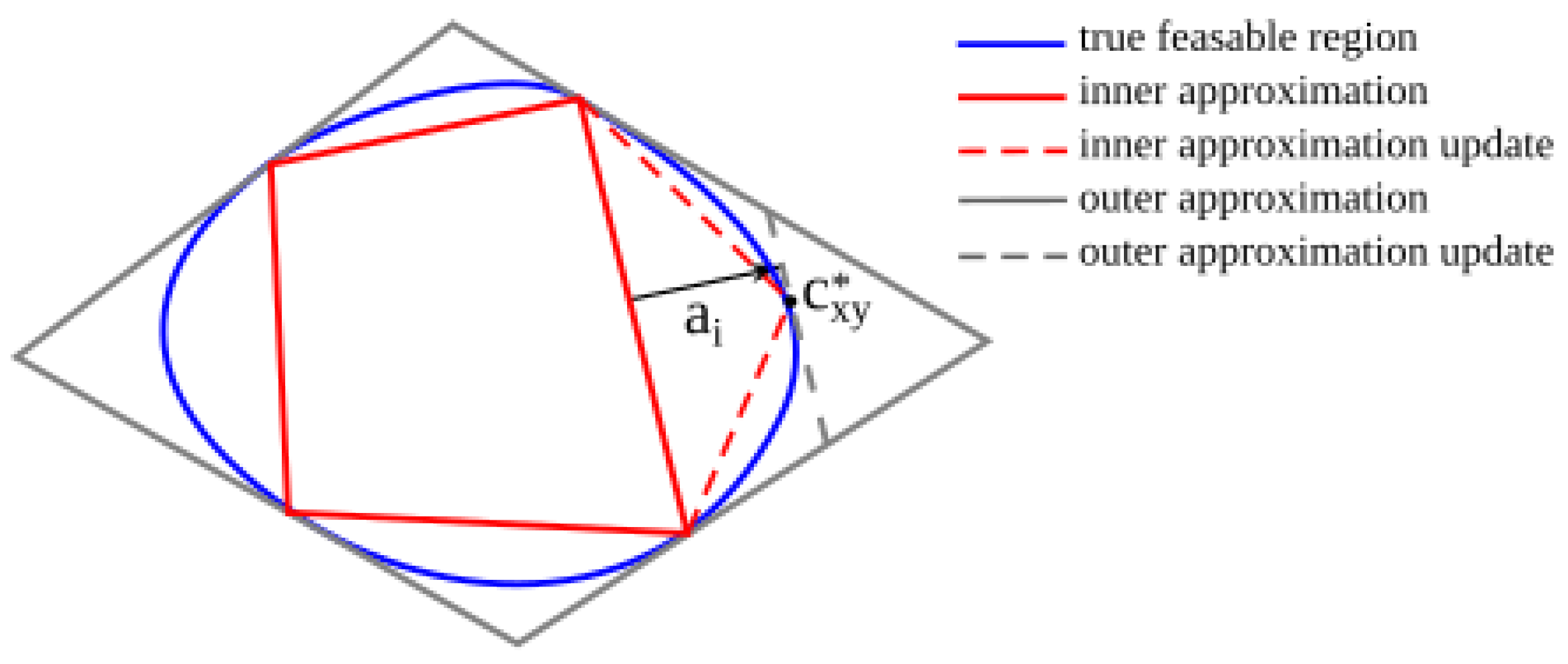
Considering all that, we decided to choose the CoM position by iteratively computing the desired CoM position and solving IK until we found a satisfactory CoM position along with a complete robot configuration. The procedure is described in Algorithm 3. In step (I), the feasible area around the current joint configuration is computed. Then, in step (II), we compute the centroid of contact positions ${\mathbf{c}}_{mid}$. After that, we go in a loop where we first find the desired position of CoM along x and y directions in step (III) by finding the closest point from the feasible region ${\mathcal{Y}}_{fa}$ to ${\mathbf{c}}_{mid,xy}$. After computing the desired CoM position, we solve the IK in step (IV). As the desired CoM motion might not be reachable, IK would lead us to the closest point to it. So in the next step (V), CoM position in x and y directions from IK is computed, followed by recomputation of the feasible region around the IK solution in step (VI). The procedure ends when the CoM position in x and y directions from IK is within ${\mathcal{Y}}_{fa}$ computed at the same robot state $\mathbf{q}$. We might apply some safety margin when checking if CoM is within a feasible region. The illustration of one step of a procedure is given in Figure 4. The big difference between two consecutive feasible regions is proof of the necessity for a described algorithm.

When computing the feasible region ${\mathcal{Y}}_{fa}$, we consider three feet that will stay in contact during the whole step. If the robot is statically balanced with three feet in contact during the swing phase, it will also be balanced with all four legs during the CoM translation phase. Conversely, when considering reachability, the CoM translation phase is more constraining, so for solving IK, we still consider all four legs.

Algorithm 3 carries out CoM motion planning while ensuring reachability by explicitly solving the IK problem. Static stability is ensured by computing the feasible region ${\mathcal{Y}}_{fa}$ for the IK solution. The enabler for this sequential procedure is the ability to efficiently compute ${\mathcal{Y}}_{fa}$.

Algorithm 3 Sequential CoM computation.

Inputs: ${\mathbf{c}}_{xy},{\mathbf{p}}_1,\cdots ,{\mathbf{p}}_{n_c},{\mathbf{S}}_1^{\mu },\cdots ,{\mathbf{S}}_{n_c}^{\mu },{\underline{\mathit{\tau }}}_1\cdots {\underline{\mathit{\tau }}}_{n_j},{\overline{\mathit{\tau }}}_1\cdots {\overline{\mathit{\tau }}}_{n_j}$ Result: Desired position of CoM in x and y directions function FindCoMXY(${\mathcal{Y}}_{fa},{\mathbf{c}}_{mid}$)        ${\mathbf{c}}_{des}=\mathrm{argmin}{\parallel {\mathbf{c}}_{xy}-{\mathbf{c}}_{mid,xy}\parallel }^2$          such that: ${\mathbf{c}}_{xy}\in {\mathcal{Y}}_{fa}$ return  ${\mathbf{c}}_{des}$ end function (I) Compute ${\mathcal{Y}}_{fa}$ using recursive IP (II) ${\mathbf{c}}_{mid}=\mathrm{mean}\left({\mathbf{p}}_1,\cdots ,{\mathbf{p}}_{n_c}\right)$ repeat      (III) ${\mathbf{c}}_{des}=\mathrm{FindComXY}\left({\mathcal{Y}}_{fa},\mathbf{d}\right)$      (IV) $\mathbf{q}=\mathrm{IK}\left({\mathbf{c}}_{des},{\mathbf{p}}_1,\cdots ,{\mathbf{p}}_{n_c}\right)$      (V) ${\mathbf{c}}_{IK}=\mathrm{ComputeCom}\left(\mathbf{q}\right)$      (VI) Compute ${\mathcal{Y}}_{fa}$ using recursive IP until  ${\mathbf{c}}_{IK}\in {\mathcal{Y}}_{fa}$ return  $c_{IK}$

4.2. Prioritized IK

The robot has 18 DoF, but only fourteen constraints are specified, with locations of four feet (three constraints per foot, twelve in total) and positions of CoM in the horizontal plane (two constraints). To fully define the IK problem, we have added two more requirements:

• The base of the robot has to be at a preset height above the instantaneous walking plane (one constraint).
• The base of the robot has to have a preset orientation relative to the instantaneous walking plane (three constraints).

With that, the IK is fully defined. We define the instantaneous walking plane as the plane with minimal distance to all contact points between the robots’ feet and the environment. Of course, if only three feet are in contact with the environment, we can compute a plane that contains all the contact points. The priority of these two tasks is lower than moving CoM or stepping while keeping feet in contact. For this reason, we have developed a constrained prioritized IK scheme. The method is given in Algorithm 4.

The input to the algorithm is a constraint and tasks with their given priorities. The task is defined by the way of computing task errors and the associated Jacobian matrix. Together with that, a robot state $\mathbf{q}$ that includes joint angles and pose of free-floating base and bounds on joint angles, lower bound $\underline{\mathbf{q}}$ and upper bound $\overline{\mathbf{q}}$ are given. The algorithm is iterative, where in each iteration, we solve a quadratic program (QP) for each task from the highest- to the lowest-priority task. QP computes an update on joint state ${\mathbf{v}}^{*}$ such that joint angles will be within joint bounds after the update (inequality constraint III.b), and it does not influence the constraint (equality constraint III.a). After computing the coordinate update in step (IV), the constraint matrix is updated in step (V) by appending the task Jacobian ${\mathbf{J}}_i$ to the constraint matrix $\mathbf{J}$. Because of that, all subsequent lower-priority tasks are solved without influencing current and all higher-priority tasks and constraints.

By giving the highest priority to CoM motion and giving everything else (base motion, EEF motion) a lower priority when solving IK, we have maximized the CoM reachability region as we pushed other tasks to be solved with lower priority.

Algorithm 4 Constrained multi-priority IK solver.

Input: Tasks with priorities, $\underline{\mathbf{q}}$, $\overline{\mathbf{q}}$ Result: Joint coordinates $\mathbf{q}$ $done=\mathrm{False}$ ${\mathbf{q}}^{*}=\mathbf{q}$ while  $\neg done$  do     $success=\mathrm{True}$     Compute constraint Jacobian ${\mathbf{J}}_C$     $\mathbf{J}={\mathbf{J}}_C,\mathbf{a}=\mathbf{0}$     for priority i in all priorities do           (I) Compute error ${\mathbf{e}}_i$           (II) Compute task Jacobian ${\mathbf{J}}_i$           (III) Solve quadratic program:            ${\mathbf{v}}^{*}=\mathrm{argmax}\parallel {\mathbf{J}}_i\mathbf{v}-{\mathbf{e}}_j\parallel$            such that:              III.a) $\mathbf{J}\mathbf{v}=\mathbf{a}$              III.b) $\underline{\mathbf{q}}\le {\mathbf{q}}^{*}+\alpha \mathbf{v}\le \overline{\mathbf{q}}$           (IV) ${\mathbf{q}}^{*}={\mathbf{q}}^{*}+\alpha {\mathbf{v}}^{*}$           (V) $\mathbf{J}={\left[{\mathbf{J}}^T{\mathbf{J}}_i^T\right]}^T$$\mathbf{a}={\left[{\mathbf{a}}^T{\left({\mathbf{J}}_i{\mathbf{v}}^{*}\right)}^T\right]}^T$           (VI) $done=done\wedge \left(\parallel {\mathbf{e}}_i\parallel <{ϵ}_e\vee \parallel {\mathbf{v}}^{*}\parallel <{ϵ}_v\right)$     end for end while return  ${\mathbf{q}}^{*}$

5. Implementation

In this section, we will go through the implementation details, allowing us to run the approach efficiently in simulation.

As previously stated, the contact sequence is given in advance, and for each segment of the motion, we have two phases:

• Moving the CoM while all four feet are in contact with the environment
• Moving the foot while CoM is stationary and the other three feet are in contact with the environment

What is common for both phases is that we have both kinematic constraints and force constraints coming from (three or four) feet in contact with the environment. While maintaining constraints, we must move some reference points (CoM or foot). Also, Solo12 is a torque-controlled robot, meaning that we are supposed to present a set of torque commands in each step. For this purpose, we have used a custom whole-body controller.

5.1. Whole-Body Controller

Whole-body control has been extensively studied by robotics research in the past. Some great examples of multi-priority whole-body controllers were presented in [29,30]. Those control schemes were able to solve multi-priority equality and inequality-constrained problems. Unfortunately, such methods require several optimization problems to be solved in each step, making them computationally inefficient. As noted in [31], it is hard to achieve the high frequencies needed for torque control when using multiple priorities. It is stated that only when using a single priority 1 kHz control loop can it be achieved. On the other hand, machine learning-based controllers cannot guarantee the fulfillment of the constraints. Hence, they cannot guarantee the static stability of the system. For these reasons, we decided to define the whole body controller as a single-priority multi-objective constrained quadratic program. The QP is as follows:

$$\begin{array}{cc}\hfill \underset{\ddot{\mathbf{q}},\mathit{\tau },{\mathbf{f}}_1\cdots {\mathbf{f}}_{{\mathrm{n}}_{\mathrm{c}}}}{min}& \parallel {\mathbf{J}}_T\ddot{\mathbf{q}}-{\mathbf{a}}_T\parallel +{\lambda }_{\mathit{\tau }}\parallel \mathit{\tau }\parallel +{\lambda }_f\sum _{i=1}^{n_c}\parallel {\mathbf{T}}_i{\mathbf{f}}_i\parallel \hfill \\ \hfill \mathrm{s}.\mathrm{t}& \mathbf{M}\ddot{\mathbf{q}}+\mathbf{C}\dot{\mathbf{q}}+\mathbf{g}=\left[\begin{array}{c}{\mathbf{0}}_{6\times n_j}\\ {\mathbf{I}}_{n_j\times n_j}\end{array}\right]\mathit{\tau }+\sum _{i=1}^{n_c}{\mathbf{J}}_i^T{\mathbf{f}}_i\hfill \\ \hfill & {\mathbf{J}}_i\ddot{\mathbf{q}}+{\dot{\mathbf{J}}}_i\dot{\mathbf{q}}=\mathbf{0},i=1\dots n_c\hfill \\ \hfill & {\mathbf{B}}_i{\mathbf{f}}_i<\mathbf{0},i=1\dots n_c\hfill \\ \hfill & \underline{\mathit{\tau }}<\mathit{\tau }<\overline{\mathit{\tau }}\hfill \end{array}$$

(7)

The objective function is composed of three parts. The first part tries to minimize deviation from the desired motion where ${\mathbf{J}}_T$ is a task Jacobian and ${\mathbf{a}}_T$ is the desired acceleration. The second term is used to minimize joint torques $\mathit{\tau }$, while the third term is used to reduce contact forces ${\mathbf{f}}_i$ multiplied by the weighing matrix ${\mathbf{T}}_i$. In the case we have considered, we were trying to minimize only forces tangential to the surface, so the weighing matrix assumes the form:

$${\mathbf{T}}_i=\left[\begin{array}{ccc}1& 0& 0\\ 0& 1& 0\end{array}\right]{\mathbf{R}}_i^T.$$

(8)

That way, we are trying to minimize the possibility of sliding.

The first equality constraint from QP given by (7) is a general equation dynamics of multi-body systems, with matrix $\mathbf{M}$ representing inertia matrix, $\mathbf{C}$ representing matrix of Coriolis and centrifugal effects and $\mathbf{g}$ is a gravitational load. The next equality constraint is a contact constraint, saying the acceleration of the contact point should be 0. The last two inequality constraints are the same as III.b and III.c from Algorithm 1, with the first one being the constraint of force coming from point contact with Coulomb friction, and the second one being a constraint on actuation torques. All Jacobians, inertia and Coriolis matrices and gravitational load were computed using Pinocchio [32], a library providing fast and efficient Rigid Body Algorithms. With ProxQP and C++ implementation, the QP is solved in less than 0.15 ms, while the computation of Jacobians and other necessary matrices in Equation (7) takes less than 0.05 ms on computer running Ubuntu 24.04 with AMD Ryzen7 5800H processor with 16 GB of ram memory. The whole-body controller can be run at even faster rates, up to 5 kHz, which is 20 times faster than the whole-body controller from [26], but we decided to go with 1 kHz due to the communication bandwidth between the PC and the real robot.

5.2. Moving CoM Phase

In this phase, the emphasis is on moving CoM while all four legs are in contact with the ground. The CoM has to follow a trajectory in 2D, the base has to keep its orientation parallel to the instantaneous walking plane, and the base has to be at a given height. Thus, the task Jacobian and desired acceleration assume the form:

$$\begin{array}{cc}\hfill {\mathbf{J}}_T& =\left[\begin{array}{c}{\mathbf{J}}_{CoM,xy}\\ \mathbf{S}{\mathbf{J}}_B\end{array}\right]\hfill \end{array}$$

(9)

$$\begin{array}{cc}\hfill {\mathbf{a}}_T& =\left[\begin{array}{c}{\mathbf{a}}_{CoM,xy}^{des}-{\dot{\mathbf{J}}}_{CoM,xy}\dot{\mathbf{q}}\\ \mathbf{D}\left({\mathbf{a}}_B^{des}-{\dot{\mathbf{J}}}_B\dot{\mathbf{q}}\right)\end{array}\right],\hfill \end{array}$$

(10)

where ${\mathbf{J}}_{CoM,xy}\in {\mathtt{R}}^{2\times 18}$ and ${\dot{\mathbf{J}}}_B\in {\mathtt{R}}^{6\times 18}$ are Jacobians associated with CoM in xy plane and translational and rotational motion of the base, respectively. Matrix $\mathbf{D}=\left[{\mathbf{0}}_{4\times 2}{\mathbf{I}}_{4\times 4}\right]\mathrm{diag}\left(R_W^T,R_W^T\right)$ rotates the base motion to instantaneous walking plane and selects just translation in z direction and rotation part by dropping the first two rows. Vectors ${\mathbf{a}}_{CoM,xy}^{des}$ and ${\mathbf{a}}_B^{des}$ are desired CoM and base accelerations. The accelerations are obtained so that those two reference points follow the defined trajectory computed during CoM motion planning. Based on the current state and output of the Sequential CoM computation, linear CoM and base trajectories are defined. Desired accelerations are computed as a combination of reference accelerations ${\mathbf{a}}^{ref}$ computed from the trajectory and PD components. The equations for both desired accelerations follow the same form:

$${\mathbf{a}}^{des}={\mathbf{a}}^{ref}+K_p\mathbf{e}+K_d\dot{\mathbf{e}}.$$

(11)

In the former equation, the tracking error is denoted by $\mathbf{e}$, while $K_p$ and $K_d$ are position and derivative gains.

As we need precise CoM motion to maintain static balance, the highest-priority task in IK during the sequential CoM computation was CoM positioning. Since having a flat base or being at some distance from the feet is not of fundamental importance, the base movement task in the IK was the second priority. Both are flattened and assigned the same priority in our whole-body controller, but with values resulting from prioritized IK, guaranteeing that the robot can fulfill both tasks.

5.3. Swing Phase

As in the previous phase in each control cycle, the optimization problem given by Equation (7) is given. The only difference is that one less contact is present, $n_c=3$, and that we need to take care of the trajectory of the foot. Before starting this phase, prioritized IK was solved once more, with CoM position and swing foot positioning having the highest priority, while base position still had lower priority. That way, we guarantee that CoM will stay at the previously computed statically stable position while reaching the foot placement at the expense of base height and orientation.

The task Jacobian, in this case, assumes the form:

$$\begin{array}{cc}\hfill {\mathbf{J}}_T& =\left[\begin{array}{c}{\mathbf{J}}_{CoM,xy}\\ \mathbf{S}{\mathbf{J}}_B\\ {\mathbf{J}}_s\end{array}\right]\hfill \end{array}$$

(12)

$$\begin{array}{cc}\hfill {\mathbf{a}}_T& =\left[\begin{array}{c}{\mathbf{a}}_{CoM,xy}^{des}-{\dot{\mathbf{J}}}_{CoM,xy}\dot{\mathbf{q}}\\ \mathbf{D}\left({\mathbf{a}}_B^{des}-{\dot{\mathbf{J}}}_B\dot{\mathbf{q}}\right)\\ {\mathbf{a}}_s^{des}-{\dot{\mathbf{J}}}_s\dot{\mathbf{q}}\end{array}\right],\hfill \end{array}$$

(13)

where s is the index of the swinging foot, the trajectory of the foot is obtained by fitting a cubic spline to an initial, intermediate, and desired location of the foot. The intermediate point is computed from the desired point and the normal to the new contact surface.

6. Experimental Results

For the experimental validation, we chose the high-torque and high-friction cases. The first one is when the robot is supposed to walk up the slope inclined at 60° degrees. In that case, frictional forces must be carefully considered to avoid sliding the feet in contact with the slope. In the other case, we consider a case where a robot walks with its front feet up a vertical wall. Besides the high frictional forces, a huge load is exerted on the back legs as they have to carry the whole weight of the robot and additionally push against the wall to avoid sliding. If we used coarse four-sided friction pyramids and robots with not enough torque, these motions would not be possible. Improved computation times of the feasible region allow us to use finer six- and eight-sided friction pyramids, making planning and control of these motions possible.

The simulation of our approach was performed using Mujoco [33], as its physics simulation engine is considered the most accurate [34]. For such a purpose and easy transfer from the sim to the real, we had to develop our infrastructure. The whole software was designed as two different ROS2 packages, where ROS2 itself was used mainly to organize the codebase, dependencies, and for visualization through RViz. The entire control stack, together with the Mujoco simulator or the real robot drivers, runs as a single ROS2 node. We kept everything running as a single process to avoid copying data, serialization/deserialization overhead, and communication delays in a typical publisher/subscriber architecture. That way, the control loop could achieve a frequency of 1 kHz. The friction coefficient set for simulation was $\mu =1$. All previously denoted algorithms are implemented in C++, using Pinocchio [35] to compute the kinematics and dynamics of Solo12 robot [28]. Solo12 is a torque-controlled, open-source modular robot. It was designed so that it can be 3D-printed and built in-house. It has 12 motors, each outputting a maximum 2.5 Nm at each joint. The robot weighs around 2 kg and its legs are approximately 20 cm long. The control and simulation model fully respected all joint and torque limits. When computing the control torques, we used six-sided friction pyramids with a friction coefficient of $0.9$. The whole control and simulation code has been disclosed at Github (https://github.com/ajsmilutin/ftn_solo, accessed on 22 April 2025).

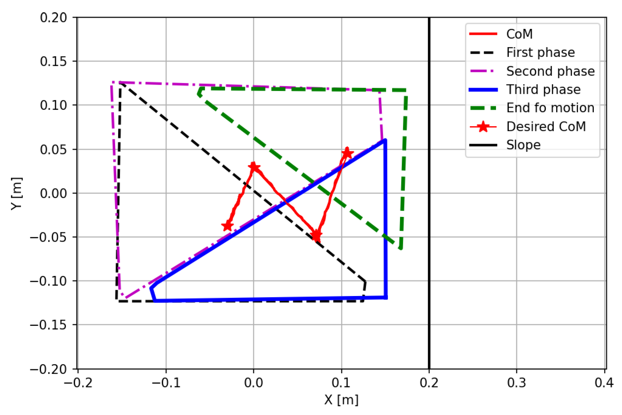
6.1. Walking Up the 60-Degree Slope

In this case, the robot should walk up the slope of ${60}^{\circ }$. As it is impossible to stand on such a slope without any adhesion, the case is tailored so that at least one of the robot’s feet is in contact with the horizontal plane (either ground or top surface). However, in such a case, high tangential friction forces are present, especially when two feet are in contact with the slope and just one with the horizontal plane. The shape of the feasible region for one segment in such a case is already depicted in Figure 4. 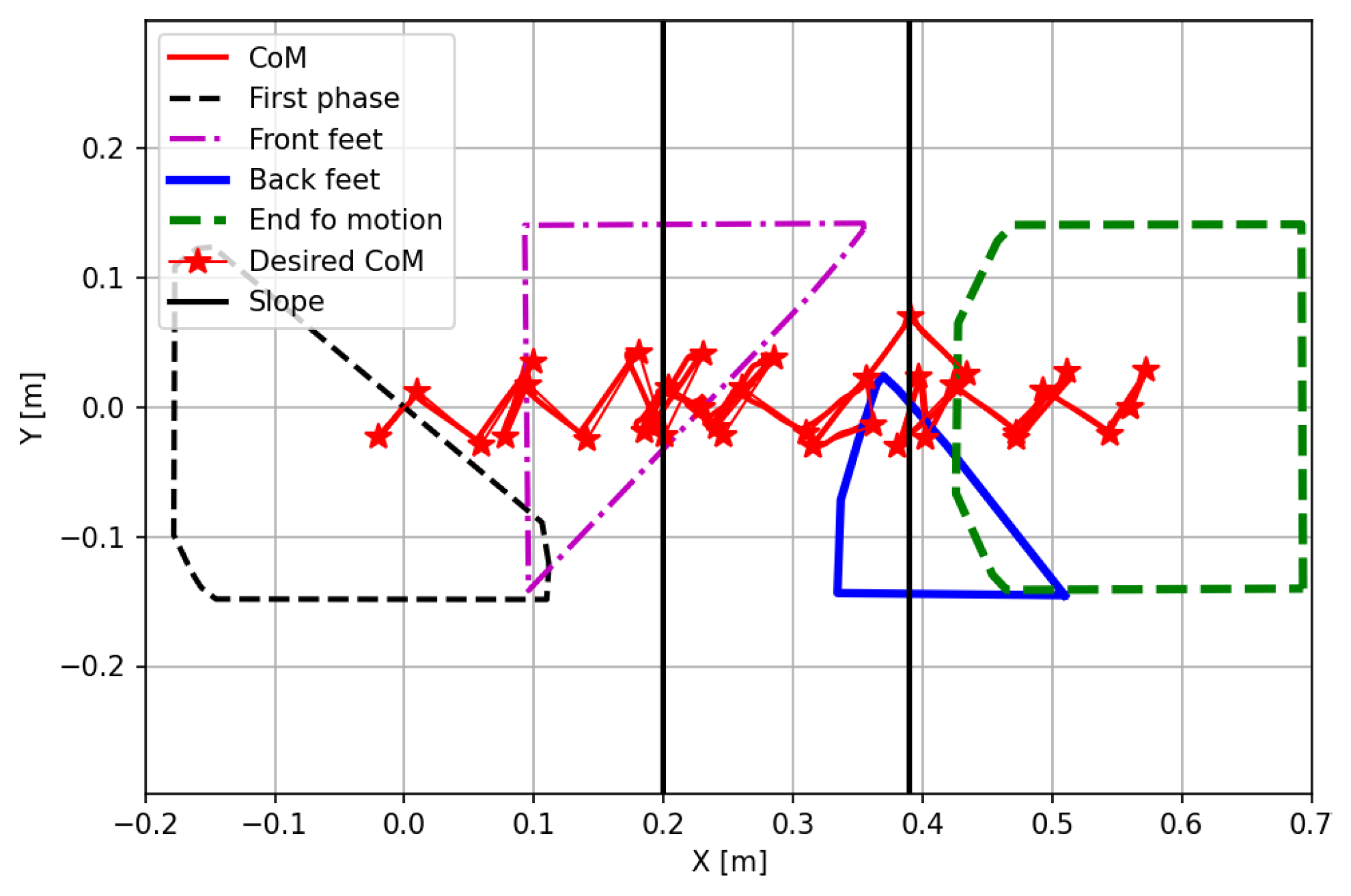Figure 5 shows the whole motion sequence. It presents the robot in four phases: the initial pose, with front feet against the slope, back feet against the slope, and the final pose. 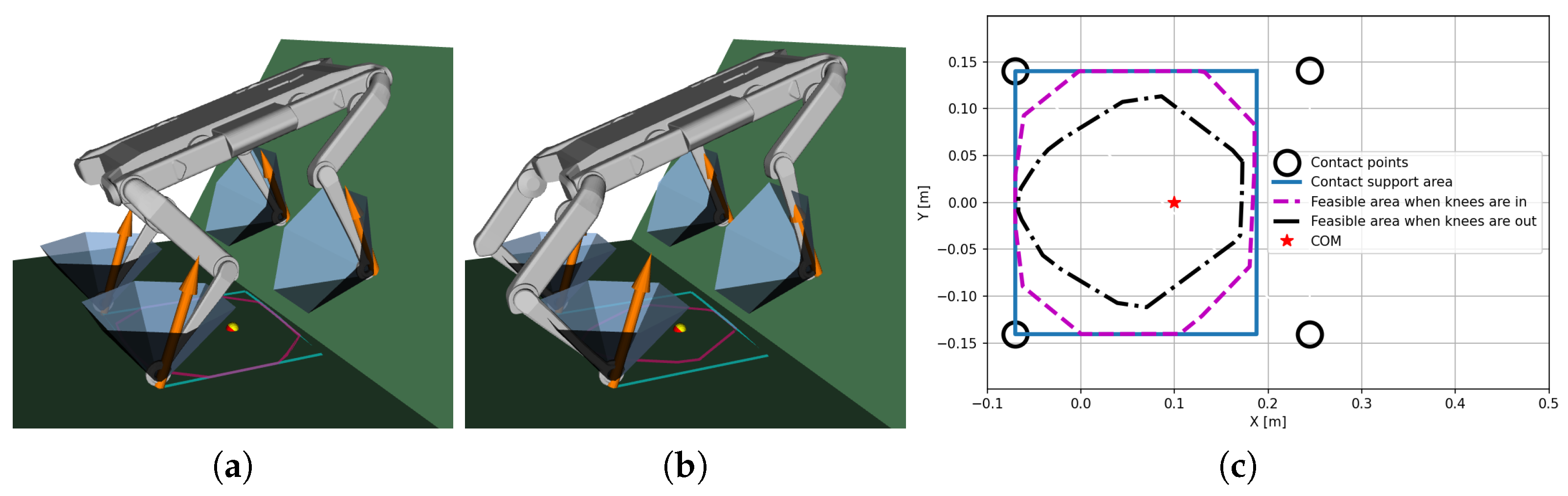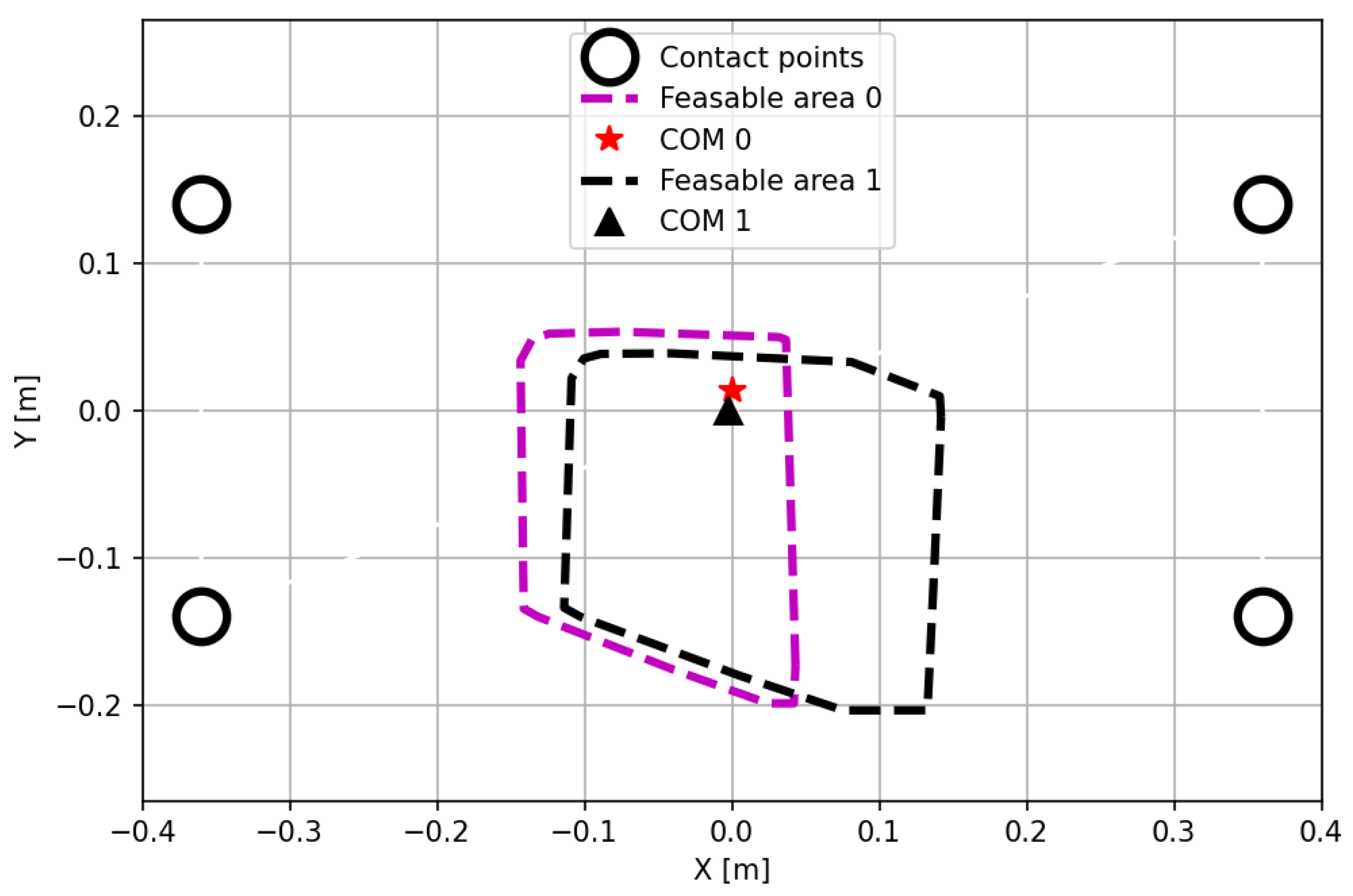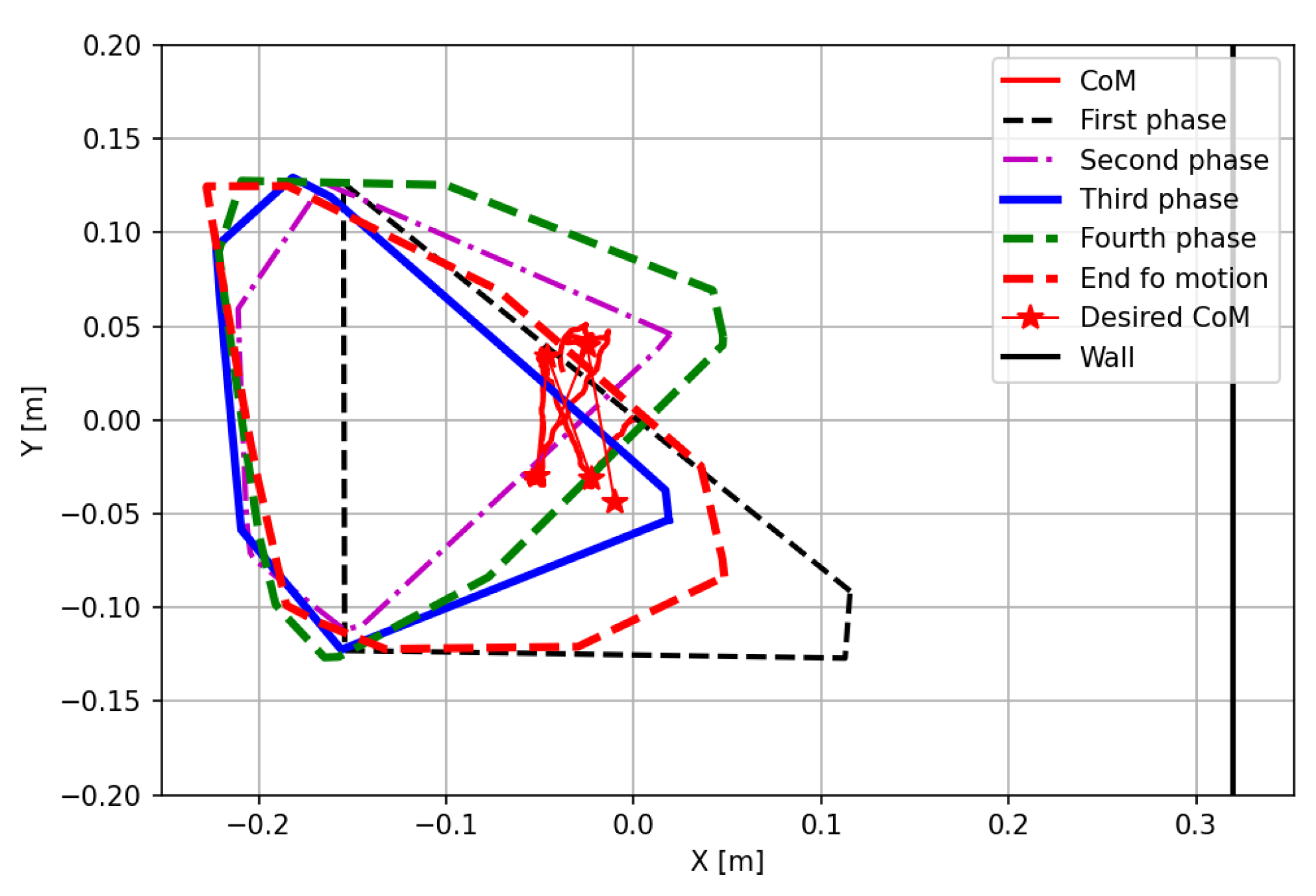Figure 6 shows the CoM trajectory and planned CoM motion, together with several feasible regions. It can be seen that feasible regions change shape and size drastically based on the phase. Also, when two back feet are in contact with the slope, and just one front foot is in contact with the top surface, the feasible region is the smallest. During one phase of the motion, the robot changes the configuration of the back knees from knees inwards to knees outwards to avoid collision with the slope.

6.2. Walking Up the Wall

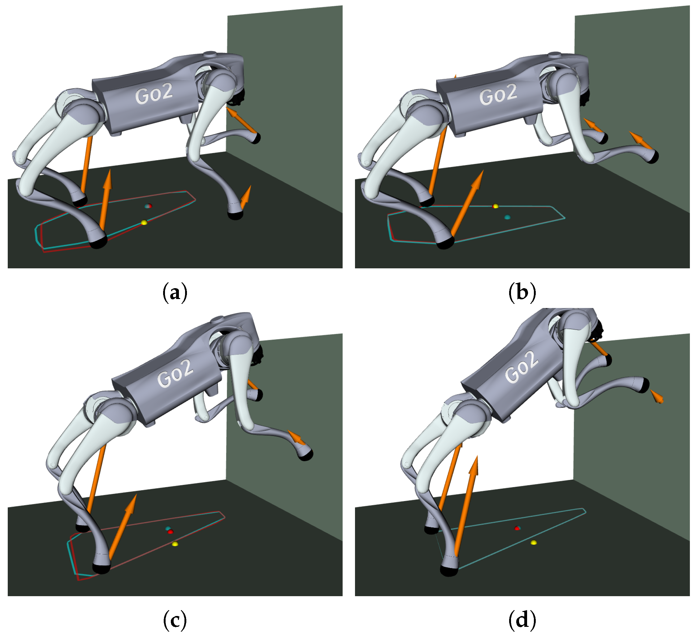
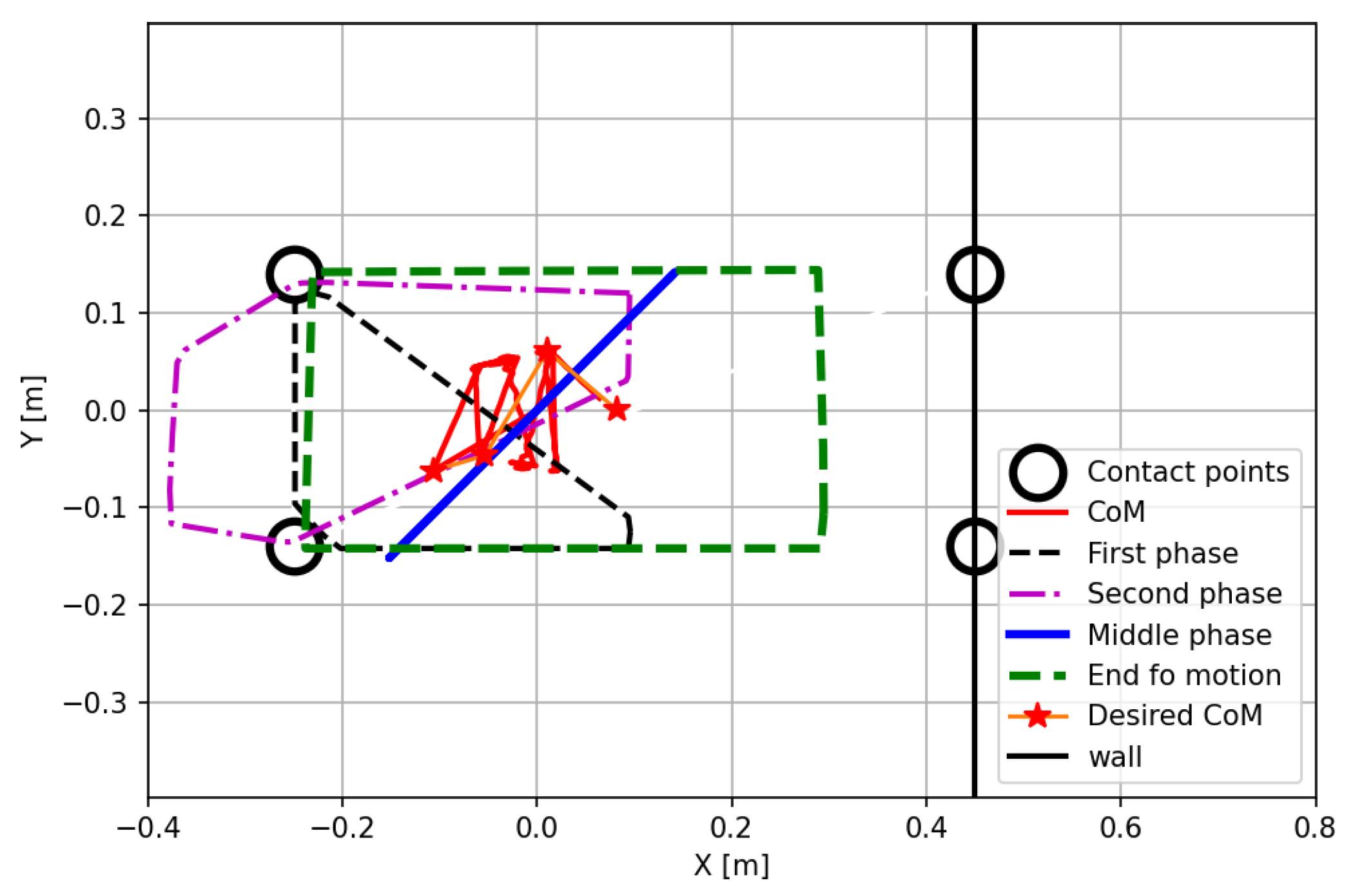
In this case, the robot is walking with its front feet up the vertical wall. This case requires high friction forces to avoid sliding. Our method only requires that the robot be torque-controlled and have four 3-degree-of-freedom legs. To prove the generality of our approach, the simulation is performed using the model of Unitree Go2 robot. That robot weighs around 15 kg with 23 Nm max joint torque, thus having a better power-to-weight ratio than Solo12. Figure 7 shows the whole motion sequence, while Figure 8 shows the CoM trajectory and planned CoM motion, together with several feasible regions. It is interesting to note that in some cases, the feasible region expands outside of the convex hull of the contact points. That contradicts the classical ZMP theory, which assumes that all contacts are in the horizontal plane.

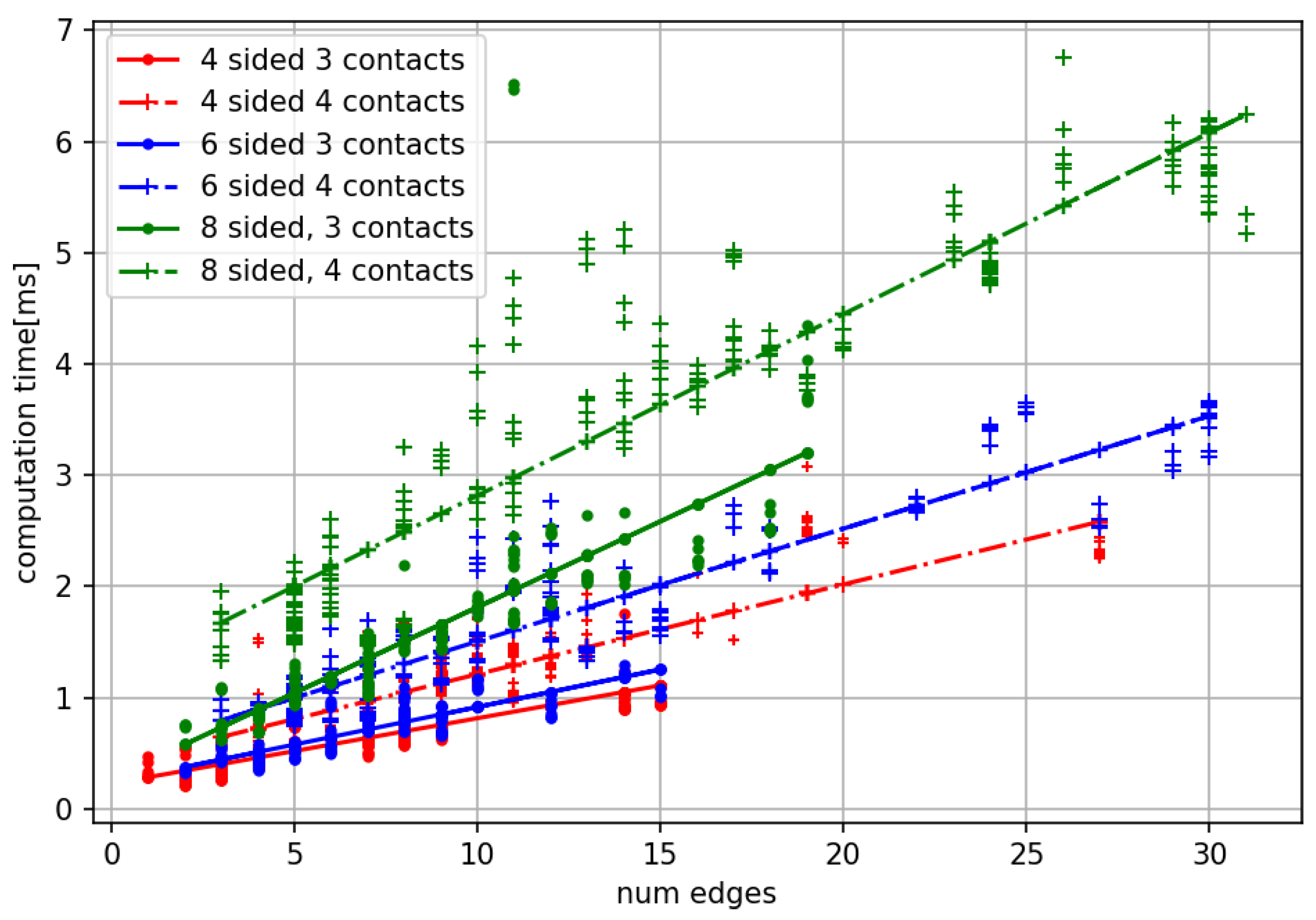
6.3. Feasible Region Computation Time

As claimed previously, this approach and implementation should provide a significant speedup when computing feasible regions. The computation times were benchmarked on the Ubuntu 24.04 running on AMD Ryzen 7 5800H processor with 16 GB of RAM. To obtain the computation time of the feasible region, we would set the number of sides in the friction pyramid and run the simulation 10 times, where in each simulation, the robot would perform 10 steps. The execution times and the number of active contacts would be logged and aggregated afterward. It is important to note that when using four-sided friction pyramids, the robot could not walk up the ramp. In that case, we would simulate walking on flat ground. The mean computation times with standard deviations of the feasible region are given in

Table 1. Mean computation time and standard deviation of feasible region using recursively expanding IP algorithm in ms.

	Number of Sides in Friction Pyramid
Num. Contacts	4	6	8
3	0.596 ± 0.299	0.692 ± 0.251	1.664 ± 0.863
4	1.288 ± 0.563	1.683 ± 0.811	3.531 ± 1.511

. From that table, several conclusions can be drawn:

• The computation time compared to the IP method described in Section 3.1 decreased around 15 times. Computation time of IP method was taken from [26], where it is stated that the average computation times for four-sided pyramids and three and four contacts are 9 ms and 14 ms, respectively.
• There are relatively big standard deviations, meaning that in some cases, computation can take much longer.
• There is a dependency on the number of contacts and sides in friction pyramids.

From the recursively expanding IP algorithm, the computation time may depend on the number of expansion steps, which directly correlates to the number of edges in the boundary of a feasible region. That correlation has been researched and plotted in Figure 9 for each entry from the previous table. From the presented figures, we can see the linear correlation between the two. Still, it depends on the number of sides in the friction pyramid and the number of contacts, which is directly related to some constraints of the optimization problem.

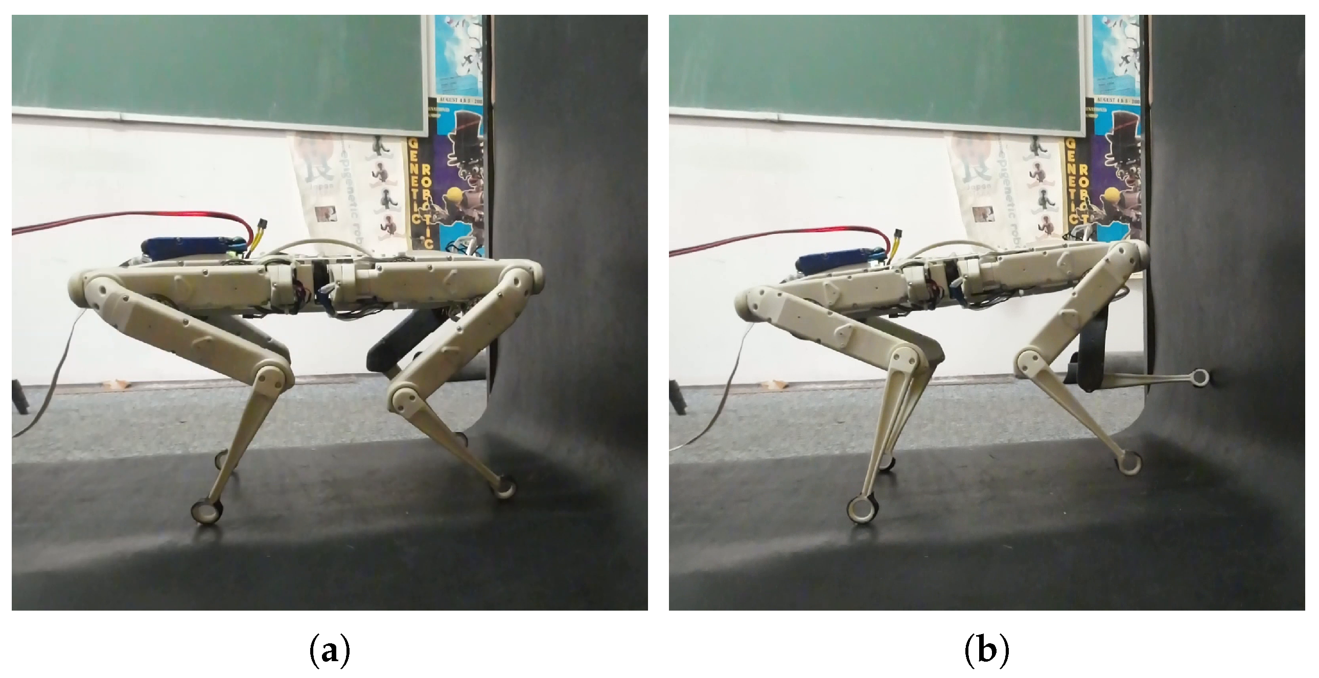
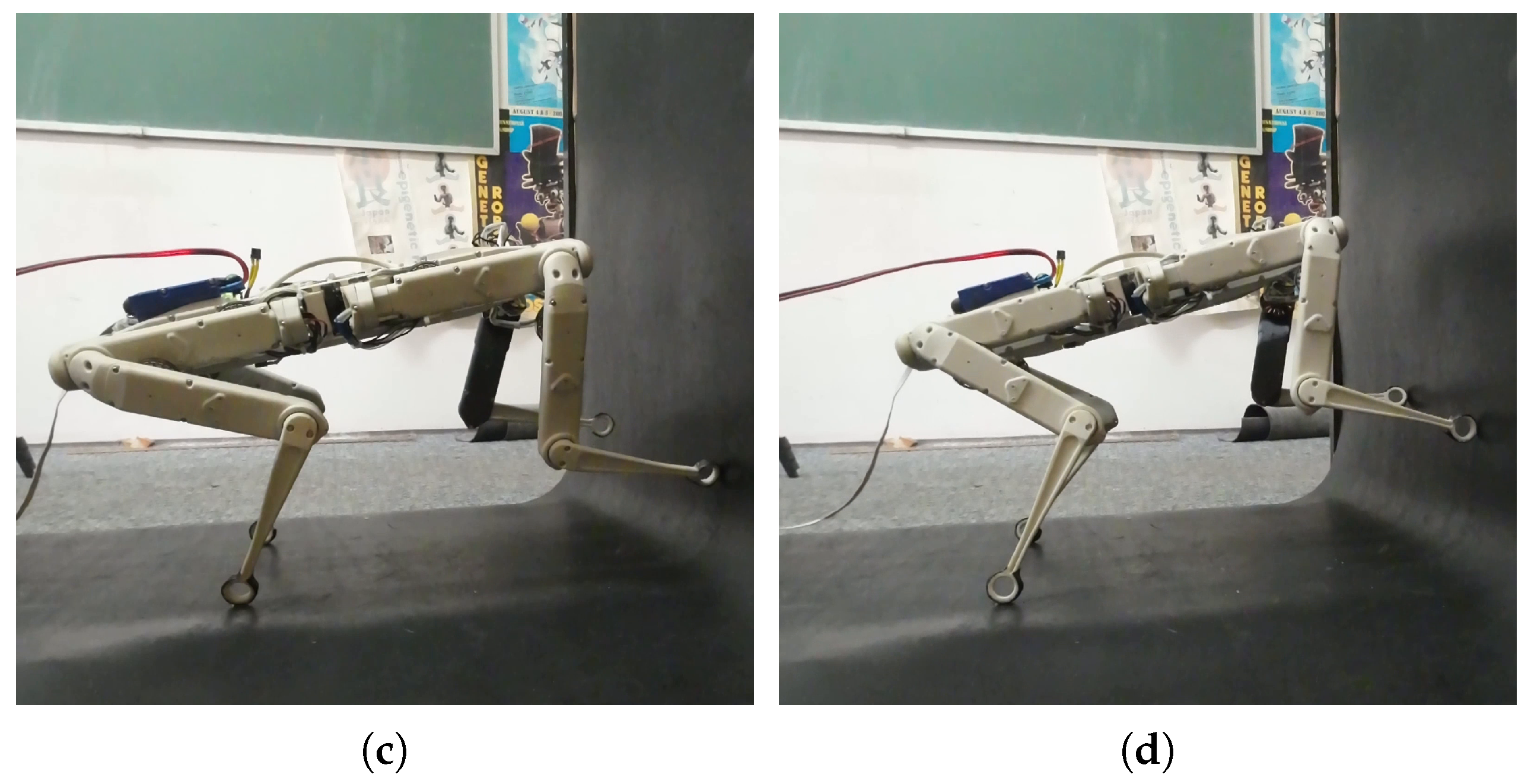
6.4. Experiments on the Real Robot

After successfully verifying our approach in the simulation, we performed experiments on the real Solo12. The experimental setup follows the simulated cases with the difference that the robot was walking up the ${45}^{\circ }$ slope. The resulting motion for walking up the slope is shown in Figure 10. CoM trajectory and feasible regions for several phases are shown in Figure 11. The resulting motion for walking up the wall is given in Figure 12, with CoM and feasible regions shown in Figure 13.

It is worth noting that on the real Solo12, we could not achieve the performance obtained in the simulation due to hardware limitations. Solo12, being mostly 3D-printed and assembled in-house, lacks the accuracy and needed stiffness. The upside of that is that the robot can be easily modified and repaired in-house. Also, we had issues with heat dissipation, as the motors used are built for quadrotors and are not suited for a high-torque low-velocity setup, as in simulated scenarios. Despite these limitations, we have shown that our method can run in real time on 1 kHz and that it is able to handle high-torque high-friction scenarios.

7. Conclusions and Future Work

In this paper, we first presented the improved IP algorithm that solves the same initial problem but, due to a change in approach, yielded a 15 × speedup, as reported in Section 6. We also tackled the reachability issue when planning a quasi-static walk by introducing iterative CoM computation coupled with a prioritized constrained IK solver. That helped us create a quasi-static walk capable of scaling the ${60}^{\circ }$ slope. The planned motion was performed using a whole-body controller running at 1 kHz. The approach was tested in a high-fidelity Mujoco simulator on a model of the Solo12 quadruped. We also ran the simulated experiment on Solo12 quadruped in our lab. As we experienced numerous hardware limitations, we hope to repeat the experiment on more mature and reliable hardware. In related works, the case of unbounded CoM acceleration was identified. We want to test the applicability of the proposed method and algorithms in such a case.

Apart from performing tests on a real robot, several other research topics were discussed. First, we plan only on the horizontal plane, but we do not plan the trajectory on the vertical plane. Except for reachability, motion in the vertical direction influences joint configurations, influencing Jacobians and limits due to joint torques. Also, in this paper, we have given a contact sequence, which opens up a problem of contact sequence planning to give the desired robot motion. With the newly adopted method, we have opened the door to faster contact sequence and motion planning, which will be part of our future research.

The biggest limitation of this method is that quasi-static motion is inherently slow, although very stable. To speed it up, we would have to consider dynamic effects and take the planning of the CoM motion more carefully. Also, the friction coefficient is unknown, but we heavily rely on it when computing the feasible region. The method for estimating friction coefficients based on visual and tactile sensor data will be necessary to mitigate this issue. The last issue we noticed is that sometimes, IK would take a long time to compute, making the motion even slower.