Energy-Coupling-Based Control for Unmanned Quadrotor Transportation Systems: Exploiting Beneficial State-Coupling Effects

Abstract

Cable suspension transport is a crucial method for quadrotors to transport goods and materials. During transportation, the quadrotor transport system (QTS) faces external disturbances and system uncertainties. Particularly, the underactuated nature of the system poses significant challenges to its stable operation. To solve these problems, this paper proposes a hierarchical control scheme that enhances coupling and leverages advantageous state-coupling to achieve precise positioning and eliminate payload swings for QTS. By leveraging the cascading characteristics of QTS, the design process is greatly simplified through the separate design of the torque input for the inner loop and the force input for the outer loop. Simulation results demonstrate the effective control performance of this method.

1. Introduction

In recent years, the quadrotor has gained significant attention, as it can achieve vertical take-off, landing, and hovering at the desired height, and high agility [1]. Various control schemes [2] and motion planning methods [3] for quadrotors have been investigated. Since the quadrotor must control translational and vertical motion as well as its attitude, it has six degrees of freedom but only four control inputs (three torques and one thrust). Thus, the system is underactuated. In addition to underactuated characteristics, strong nonlinearity, system uncertainty, external interference, and singularity are problems to be addressed when developing quadrotor controllers. To solve the issues above, adaptive nonlinear control [4], robust control [5], LQR control [6] and sliding mode control [7] were proposed for the quadrotor system. Quadrotor transportation systems, comprising quadrotors, cables, and payloads, play a crucial role in military operations and emergency response [8]. Only four control inputs are equipped in the quadrotor transportation systems to control eight DOFs, including three translational DOFs, two payload swing DOFs, and three attitude DOFs. Therefore, quadrotor transportation systems have double underactuated characteristics [9]. The underactuated characteristics, external interference, and system uncertainty bring great challenges to the control task execution of the QTS.

To track the quadrotor attitude and payload position, QTSs are always considered differential flat hybrid systems [10]. The running trajectory was planned with the geometric controller in the flat space where the payload was treated as interference when modeling [11]. Enforcing the quadrotor to the desired position may cause the payload to swing severely [12]. Open-loop [13,14,15,16,17] and closed-loop [18,19] control methods were proposed to suppress the swing problem. Closed-loop control methods demonstrate better robustness than open-loop methods by using real-time feedback signals to counter external disturbances. The nested saturation method introduced in [18] not only suppresses payload swing but also drives the quadrotor to the desired position. However, this method considers the quadrotor’s attitude as the control input and overlooks that the attitude of the quadrotor is a controlled variable, regulated by torque. A layered control method is proposed for the three-dimensional control of eight degrees of freedom to ensure body positioning, attitude control, and payload swing elimination [20]. However, due to insufficient payload information, the transient characteristics of the system cannot be guaranteed. In addition, the coupling terms in the layered control method will affect the transient characteristics of QTS, such as quadrotor position, quadrotor attitude, and payload angle.

Recently, energy-shaping methods [21,22,23] have been widely researched and used to control various mechanical systems, such as overhead cranes [24,25,26], mobile inverted pendulums [22], etc. The introduction of kinetic energy in the total energy-shaping method [27,28,29,30] enhances internal coupling and significantly improves transient characteristics compared to the potential energy shaping method [31]. However, the energy shaping method shows minimal improvement in the anti-swing effect. Introducing payload displacement information and enhancing coupling reduces the load swing angle [32]. However, the coupling term between internal attitude changes and the outer loop position continues to impact the system’s transient performance.

This paper presents a QTS control scheme based on energy shaping and beneficial coupling technology. The research utilizes a comprehensive three-dimensional model with eight degrees of freedom (DOFs) for quadrotor transportation systems using the Lagrange equation. Based on cascade system theory, the inner and outer loop controllers can be designed separately, ensuring system stability as long as the growth constraints of the coupling terms are satisfied. The inner loop uses an attitude-tracking controller [33], while the outer loop employs a new energy-coupling-based controller to manage the quadrotor’s displacement and eliminate payload swing, leveraging the beneficial coupling between the loops. Specifically, by mathematically relating body position to payload swing angle information, the swing angle is transformed into generalized displacement information. This transforms the targets of body positioning and payload swing elimination into system-wide positioning objectives. An energy storage function, incorporating both kinetic and potential energy of QTS, is established. On the basis of this function, a controller is designed to achieve precise body positioning and payload elimination. In addition, to make full use of the state coupling between the inner and outer loop subsystems, the state coupling effect is introduced. Simulation results indicate that the proposed control method outperforms the energy-coupling control method in positioning and eliminating the swing of the outer loop and enhances the attitude adjustment of the inner loop. Additionally, the results demonstrate the strong robustness of the proposed control method. Simulation results further confirm the feasibility and effectiveness of the proposed control scheme. In summary, this paper’s contributions are as follows.

(1) The newly constructed passivity property includes the quadrotor’s position information and payload swing signals, significantly enhancing state coupling compared to the energy-coupling hierarchical control method [32].

(2) In contrast to the traditional method, which directly cancels coupling terms, the proposed controller in this paper preserves beneficial coupling [34], significantly enhancing the system’s transient characteristics.

(3) When beneficial coupling exists between the inner and outer loops, the Lyapunov candidate function is discussed separately, and the theoretical proof of the asymptotic stability of the closed-loop system’s equilibrium point is provided.

2. Dynamics of the Quadrotor Transportation System

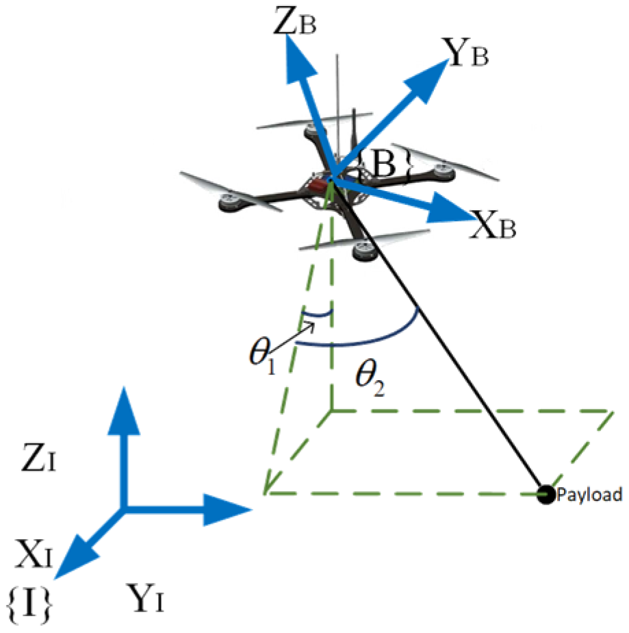
According to the QTS shown in Figure 1, the dynamic model using Euler–Lagrange equations is developed as follows:

$$M_c(q)\ddot{\mathit{q}}+V_c(\mathit{q},\dot{\mathit{q}})\dot{\mathit{q}}+\mathit{G}(\mathit{q})=\mathit{u}+{\mathit{F}}_r$$

(1)

$$\dot{\mathit{R}}=\mathit{R}sk(\mathbf{\omega })$$

(2)

$$\mathit{J}\dot{\mathit{\omega }}+sk(\mathit{\omega })\mathit{J}\mathit{\omega }=\mathit{\tau }$$

(3)

where (1) represents the outer loop dynamics model, which includes quadrotor displacement and payload swing; (2) and (3) represent the dynamics model of the inner loop, showing the attitude characteristics. $sk(\cdot ):{\mathbb{R}}^3\to so(3)$ transform a vector into a skew-symmetric matrix. $\mathit{q}(t)\in {\mathbb{R}}^5$ represents the state vector containing the body displacement and the payload swing Angle, and ${\mathit{M}}_c(\mathit{q}), {\mathit{V}}_c(\mathit{q},\dot{\mathit{q}})\in {\mathbb{R}}^{5\times 5}$ represents the inertia matrix, the centripetal-Coriolis matrix, $\mathit{G}(\mathit{q})\in {\mathbb{R}}^5$ is the gravity vector, and $\mathit{u}(\mathit{q})\in {\mathbb{R}}^5$ represents control input, and ${\mathit{F}}_r$ represents the air resistance vector, respectively. The above symbols are expressed in detail as follows:

$$\mathit{q}={[{\mathit{\xi }}^T,{\theta }_1,{\theta }_2]}^T$$

(4)

$${\mathit{M}}_c=\left[\begin{array}{ccccc}M+m& 0& 0& ml{C}_1{C}_2& -ml{S}_1{S}_2\\ 0& M+m& 0& 0& ml{C}_2\\ 0& 0& M+m& ml{S}_1{C}_2& ml{C}_1{S}_2\\ ml{C}_1{C}_2& 0& ml{S}_1{C}_2& m{l}^2{C}_2^2& 0\\ -ml{S}_1{S}_2& ml{C}_2& ml{C}_1{S}_2& 0& m{l}^2\end{array}\right]$$

(5)

$${\mathit{V}}_c=\left[\begin{array}{ccccc}0& 0& 0& -ml{\dot{\theta }}_x{S}_x{C}_y-ml{\dot{\theta }}_y{C}_x{S}_y& -ml{\dot{\theta }}_x{C}_x{S}_y-ml{\dot{\theta }}_y{S}_x{C}_y\\ 0& 0& 0& 0& -ml{\dot{\theta }}_y{S}_y\\ 0& 0& 0& ml{\dot{\theta }}_x{C}_x{C}_y-ml{\dot{\theta }}_y{S}_x{S}_y& -ml{\dot{\theta }}_x{S}_x{S}_y+ml{\dot{\theta }}_y{C}_x{C}_y\\ 0& 0& 0& -m{l}^2{\dot{\theta }}_y{C}_y{S}_y& -m{l}^2{\dot{\theta }}_x{C}_y{S}_y\\ 0& 0& 0& m{l}^2{\dot{\theta }}_x{C}_y{S}_y& 0\end{array}\right]$$

(6)

$$\mathit{G}={[0,0,0,mgl{S}_1{C}_2,mgl{C}_1{S}_2]}^T$$

(7)

$$\mathit{u}={[{(fR{e}_3-(M+m)g{e}_3)}^T,0,0]}^T$$

(8)

$$e_3={[0,0,1]}^T$$

(9)

$${\mathit{F}}_r={[f_{rx}, f_{ry}, f_{rz}, f_{r{\theta }_x}, f_{r{\theta }_y}]}^T$$

(10)

$$f_{rx}=-d_x\dot{x}-d_p\dot{x}-d_{p}l{\dot{\theta }}_1{C}_1{C}_2+d_{p}l{\dot{\theta }}_2{S}_1{S}_2$$

(11)

$$f_{ry}=-d_y\dot{y}-d_p\dot{y}-d_{p}l{\dot{\theta }}_2{C}_2$$

(12)

$$f_{rz}=-d_z\dot{z}-d_p\dot{z}-d_{p}l{\dot{\theta }}_1{S}_1{C}_2-d_{p}l{\dot{\theta }}_2{C}_1{S}_2$$

(13)

$$f_{r{\theta }_x}=-d_{p}l(\dot{x}{C}_1+\dot{z}{S}_1+l{\dot{\theta }}_1{C}_2)C_2$$

(14)

$$f_{r{\theta }_y}=-d_{p}l(-\dot{x}{S}_1{S}_2+\dot{y}{C}_2+\dot{z}{C}_1{S}_2+l{\dot{\theta }}_2)$$

(15)

where $\mathit{\xi }(t)={[x(t),y(t),z(t)]}^T\in {\mathbb{R}}^3$ represents the position of the quadrotor’s center of mass in the inertial coordinate system; ${\theta }_1(t)\in \mathbb{R}$ and ${\theta }_2(t)\in \mathbb{R}$ are the motion of the projection signal; $f(t)$ is the system control input; $R(t)\in SO(3)$ is the rotation matrix of the quadrotor from the coordinate frame to the inertial coordinate frame; $\mathit{\omega }(t)\in {\mathbb{R}}^3$ represents the quadrotor’s angular velocity when its attitude changes in the body coordinate system; $M\in \mathbb{R}$ represents the quadrotor mass; $m\in \mathbb{R}$ represents the payload mass; $l\in \mathbb{R}$ is the rope length between the quadrotor and the payload; $g\in \mathbb{R}$ is the gravitational acceleration; $J\in {\mathbb{R}}^{3\times 3}$ is the inertia moment of the quadrotor in the body coordinate system; $C_1, C_2, S_1$ and $S_2$ are abbreviations of $\cos ({\theta }_1), \cos ({\theta }_2), \sin ({\theta }_1)$, and $\sin ({\theta }_2)$, respectively.

As mentioned above, there are two main control objectives of the quadrotor lifting system, which are to ensure the quadrotor approaches the target position ${\mathit{\xi }}_d={[x_d,y_d,z_d]}^T\in {\mathbb{R}}^3$ accurately and to suppress the payload swing $\mathit{\xi }\to {\mathit{\xi }}_d, \mathbf{\Theta }\to {\mathbf{0}}_{2\times 1}$ with $\mathbf{\Theta }={[{\theta }_1,{\theta }_2]}^T$. Considering the desired position ${\mathit{q}}_d={[{\mathit{\xi }}_d^T,0,0]}^T$, the targets can also be expressed in the following:

$$\underset{t\to \infty }{\lim }(\mathit{q}-{\mathit{q}}_d)=0$$

(16)

To facilitate subsequent controller analysis and design, the outer loop tracking error ${\mathit{e}}_q(t),{\mathit{e}}_{\dot{q}}(t)\in {\mathbb{R}}^5$ is defined as follows:

$${\mathit{e}}_q(t)=\mathit{q}(t)-{\mathit{q}}_d={[e_{\xi }{(t)}^T,{\theta }_1(t),{\theta }_2(t)]}^T$$

(17)

$${\dot{\mathit{e}}}_q={[{\dot{\mathit{e}}}_{\mathit{\xi }}^T,{\dot{\mathbf{\Theta }}}^T]}^T={[{\dot{\mathit{\xi }}}^T,{\dot{\mathbf{\Theta }}}^T]}^T$$

(18)

Then, the outer loop dynamics (1) can be obtained:

$${\dot{\mathit{e}}}_q={\mathit{e}}_{\dot{q}}$$

(19)

$${\dot{\mathit{e}}}_{\dot{q}}=M_c^{-1}(\mathit{u}-V_c{e}_{\dot{q}}-\mathit{G})$$

(20)

Considering the input $\mathit{u}$ of the subsystem, the coupling term of the system through the rotation matrix $R(t)$ is a cascade form. Therefore, $fR{e}_3$ can be decomposed as follows:

$$\begin{array}{ll}fR{\mathit{e}}_3=& {\displaystyle \frac{f}{{\mathit{e}}_3^T{R}_d^{T}R{\mathit{e}}_3}}[({\mathit{e}}_3^T{R}_d^{T}R{\mathit{e}}_3)R{\mathit{e}}_3-R_d{\mathit{e}}_3]\\ & +{\displaystyle \frac{f}{{\mathit{e}}_3^T{R}_d^{T}R{\mathit{e}}_3}}{R}_d{\mathit{e}}_3\end{array}$$

(21)

$\mathbf{\Delta }\in {\mathbb{R}}^3$ contains the thrust and rotation matrix information, serving as the coupling term between the inner and outer loops. The control vector ${\mathit{f}}_d={[f_{d1},f_{d2},f_{d3}]}^T\in {\mathbb{R}}^3$, to be designed later, is defined as follows:

$$\mathbf{\Delta }={\displaystyle \frac{f}{{\mathit{e}}_3^T{R}_d^{T}R{\mathit{e}}_3}}[({\mathit{e}}_3^T{R}_d^{T}R{\mathit{e}}_3)R{\mathit{e}}_3-R_d{\mathit{e}}_3]$$

(22)

$${\mathit{f}}_d={\displaystyle \frac{f}{{\mathit{e}}_3^T{R}_d^{T}R{\mathit{e}}_3}}{R}_d{\mathit{e}}_3$$

(23)

Furthermore, the outer loop subsystem input $\mathit{u}(t)$ can be decomposed into the following three parts:

$$\mathit{u}={\mathit{u}}_d-{\mathit{m}}_0+{\mathbf{\Delta }}_d$$

(24)

where ${\mathit{u}}_d\in {\mathbb{R}}^5$ comes from the virtual control input ${\mathit{f}}_d$, ${\mathit{m}}_0\in {\mathbb{R}}^5$ represents the vector form of the combined gravity of the quadrotor and the payload, ${\mathbf{\Delta }}_d\in {\mathbb{R}}^5$ is the coupling term of the inner and outer loop, meanwhile, ${\mathbf{\Delta }}_d$ is the vector expansion form of $\mathbf{\Delta }$, which is expressed as follows:

$${\mathit{u}}_d={[{\mathit{f}}_d^T,0,0]}^T$$

(25)

$${\mathit{m}}_0={[0,0,(M+m)g,0,0]}^T$$

(26)

$${\mathbf{\Delta }}_d=[{\mathbf{\Delta }}^T,0,0]$$

(27)

According to (1), the second-order time derivative of the equation (17) can be arranged into:

$${\ddot{\mathit{e}}}_q={\mathit{M}}_c^{-1}({\mathit{u}}_d-{\mathit{u}}_m-{\mathit{V}}_c{\dot{\mathit{e}}}_q-\mathit{G})+{\mathit{M}}_c^{-1}{\mathbf{\Delta }}_d$$

(28)

A new outer loop error vector $\mathit{e}(t)\in {\mathbb{R}}^{10}$ is defined as $\mathit{e}(t)={[{\mathit{e}}_q^T(t), {\dot{\mathit{e}}}_q^T(t)]}^T$, and its derivative with respect to time can be obtained:

$$\dot{\mathit{e}}=\alpha (e,f_d,{\mathit{\xi }}_d)+\mathit{\eta }$$

(29)

where the auxiliary vector $\alpha (t)\in {\mathbb{R}}^{10}$ and coupling term $\mathit{\eta }(t)\in {\mathbb{R}}^{10}$ are given as follows:

$$\alpha ={\mathbf{\Pi }}_{10}{\dot{e}}_q+{\mathbf{\Pi }}_{01}{M}_c^{-1}(u_d-u_m-V_c{\dot{e}}_q-G)$$

(30)

$$\mathit{\eta }={\mathbf{\Pi }}_{01}{M}_c^{-1}{\mathbf{\Delta }}_d$$

(31)

where the matrices ${\mathbf{\Pi }}_{10},{\mathbf{\Pi }}_{01}\in {\mathbb{R}}^{10\times 5}$ are defined as:

$${\mathbf{\Pi }}_{10}=\left[\begin{array}{c}{I}_{5\times 5}\\ 0_{5\times 5}\end{array}\right],{\mathbf{\Pi }}_{01}=\left[\begin{array}{c}{0}_{5\times 5}\\ I_{5\times 5}\end{array}\right]$$

(32)

with $I_{5\times 5}$ representing the identity matrix and $0_{5\times 5}$ representing the zero matrix.

The attitude error ${\mathit{e}}_R\in {\mathbb{R}}^3$ and angular velocity error ${\mathit{e}}_{\omega }\in {\mathbb{R}}^3$ in the inner loop subsystem are defined as follows:

$${\mathit{e}}_R={\displaystyle \frac{1}{2}}\mathrm{v}\mathrm{e}\mathrm{x}({\mathit{R}}_d^T\mathit{R}-{\mathit{R}}^T{\mathit{R}}_d)$$

(33)

$${\mathit{e}}_{\omega }=\mathit{\omega }-{\mathit{R}}^T{\mathit{R}}_d{\mathit{\omega }}_d$$

(34)

where $\mathrm{v}\mathrm{e}\mathrm{x}(\cdot ):\mathrm{s}\mathrm{o}(3)\to {\mathbb{R}}^3$ is the inverse operation of $sk(\cdot )$, ${\mathit{R}}_d\in {\mathbb{R}}^{3\times 3}$ is the desired attitude, ${\mathit{\omega }}_d\in {\mathbb{R}}^3$ is the quadrotor’s angular velocity in the body coordinate system. The time derivatives of ${\mathit{e}}_R$ and ${\mathit{e}}_{\omega }$ are as follows:

$${\dot{\mathit{e}}}_R={\displaystyle \frac{1}{2}}\mathrm{v}\mathrm{e}\mathrm{x}({\mathit{R}}_d^T\mathit{R}\mathrm{s}\mathrm{k}({\mathit{e}}_{\omega })+\mathrm{s}\mathrm{k}({\mathit{e}}_{\omega }){\mathit{R}}^T{\mathit{R}}_d))$$

(35)

$$\mathit{J}{\dot{\mathit{e}}}_{\omega }=\mathit{\tau }-sk(\mathit{\omega })\mathit{J}\mathit{\omega }+\mathit{J}(sk(\mathit{\omega }){\mathit{R}}^T{\mathit{R}}_d{\mathit{\omega }}_d-{\mathit{R}}^T{\mathit{R}}_d{\dot{\mathit{\omega }}}_d)$$

(36)

Then, a nonlinear control scheme is designed for the QTS of (17), (18), (33), and (34) to achieve the control objective.

Remark 1. 

The four control inputs composed of $f\in \mathbb{R}$ and $\mathit{\tau }\in {\mathbb{R}}^3$ and the controlled variables composed of displacement and attitude make the system an underactuated system and make QTS have ‘double’ underactuated characteristics after the introduction of the payload. Unlike fully actuated systems, in this case, the outer loop control input $\mathit{u}(t)$ influences both thrust $f(t)$ and torque $\mathit{\tau }(t)$, which in turn affects the inner loop attitude $\mathit{R}(t)$. There is a coupling between attitude adjustment in the inner loop and control inputs in the outer loop.

For the convenience of subsequent analysis, (1) is expanded and transformed as follows:

$$(M+m)\ddot{x}+ml({\ddot{\theta }}_1{C}_1{C}_2-{\ddot{\theta }}_2{S}_1{S}_2-{\dot{\theta }}_1^2{S}_1{C}_2-{\dot{\theta }}_2^2{S}_1{C}_2-2{\dot{\theta }}_1{\dot{\theta }}_2{C}_1{S}_2)=f{R}_{13}$$

(37)

$$(M+m)\ddot{y}+ml({\ddot{\theta }}_2{C}_2-{\dot{\theta }}_2^2{S}_2)=f{R}_{23}$$

(38)

$$(M+m)\ddot{z}+ml({\ddot{\theta }}_1{S}_1{C}_2+{\ddot{\theta }}_2{C}_1{S}_2+{\dot{\theta }}_1^2{C}_1{C}_2+{\dot{\theta }}_2^2{C}_1{C}_2-2{\dot{\theta }}_1{\dot{\theta }}_2{S}_1{S}_2)=f{R}_{33}-(M+m)g$$

(39)

$$\ddot{x}{C}_1{C}_2+(\ddot{z}+g)S_1{C}_2+l{\ddot{\theta }}_1{C}_2^2-2l{\dot{\theta }}_1{\dot{\theta }}_2{C}_2{S}_2=0$$

(40)

$$\ddot{x}{S}_1{S}_2-\ddot{y}{C}_2-(\ddot{z}+g)C_1{S}_2-l{\ddot{\theta }}_2-l{\dot{\theta }}_1^2{C}_2{S}_2=0$$

(41)

3. Energy Storage Function Construction

In this section, the characteristics of position signals are analyzed in detail and a new energy storage function is proposed.

For the outer loop subsystem, the energy equation is derived using the system’s kinetic and potential energy as follows:

$$E={\displaystyle \frac{1}{2}}{\dot{\mathit{q}}}^T{\mathit{M}}_c\dot{\mathit{q}}+mgl(1-C_1{C}_2)$$

(42)

Since ${\mathit{M}}_c$ is a positive-definite symmetric matrix, $E$ is locally positive definite with respect to $\dot{\mathit{q}}(t), {\theta }_1(t)$, and ${\theta }_2(t)$. Taking the time derivative of (42), and considering that ${\dot{\mathit{M}}}_c-2{\mathit{V}}_c$ is a skew-symmetric matrix, one obtains that

$$\begin{array}{ll}\dot{E}& ={\dot{\mathit{q}}}^T({\mathit{M}}_c\ddot{\mathit{q}}+{\displaystyle \frac{1}{2}}{\dot{\mathit{M}}}_c\dot{\mathit{q}})+mgl({\dot{\theta }}_1{S}_1{C}_2+{\dot{\theta }}_2{C}_1{S}_2)\\ & ={\dot{\mathit{\xi }}}^T[f\mathit{R}{\mathit{e}}_3-(M+m)g{\mathit{e}}_3]\end{array}$$

(43)

The above formula shows that $f\mathit{R}{\mathit{e}}_3-(M+m)g{\mathit{e}}_3$ is the system input and $\mathit{\xi }$ is the system output. Since the payload information $\mathbf{\Theta }(t), \dot{\mathbf{\Theta }}(t)$ is underactuated, it is not included in $E$. Therefore, $E(t)$ is only related to the displacement $\mathit{\xi }(t)$ of the quadrotor. Then, payload information is introduced to reshape the energy equation. The payload position is expressed as follows:

$${\mathit{\xi }}_p=\mathit{\xi }+l{[S_1{C}_2, S_2,-C_1{C}_2]}^T$$

(44)

The following generalized displacement signal is introduced:

$${\mathit{\chi }}_p=\mathit{\xi }+\mathit{h}(\mathbf{\Theta })$$

(45)

where $\mathit{h}={[h_1, h_2, h_3]}^T$ is the undetermined coefficient related to the payload swing. Then a new energy storage function $E_k(t)$ is defined utilizing the generalized displacement signal ${\mathit{\chi }}_p$, and its derivative can be written as:

$$\begin{array}{ll}{\dot{E}}_k(t)& ={\dot{\mathit{\chi }}}_p^T[f\mathit{R}{\mathit{e}}_3-(M+m)g{\mathit{e}}_3]\\ & ={(\dot{\mathit{\xi }}+\dot{\mathit{h}})}^T[f\mathit{R}{\mathit{e}}_3-(M+m)g{\mathit{e}}_3]\end{array}$$

(46)

Direct control of load-induced generalized displacement enhances the coupling between displacement and payload movement in the quadrotor.

To determine the specific expression of $E_k(t)$, we know from (42), (43), and (46)

$$E_k=E+E_d$$

(47)

where $E_d(t)$ is obtained by

$${\dot{E}}_d={\dot{\mathit{h}}}^T[f\mathit{R}{\mathit{e}}_3-(M+m)g{\mathit{e}}_3]$$

(48)

Substituting (37)–(39) into (48), we have

$${\dot{E}}_d={\dot{E}}_{dx}+{\dot{E}}_{dy}+{\dot{E}}_{dz}$$

(49)

The specific form of ${\dot{E}}_{dx}$, ${\dot{E}}_{dy}$, and ${\dot{E}}_{dz}$ are as follows:

$$\begin{array}{ll}{\dot{E}}_{dx}=& ({\displaystyle \frac{\partial h_1}{\partial {\theta }_1}}{\dot{\theta }}_1+{\displaystyle \frac{\partial h_1}{\partial {\theta }_2}}{\dot{\theta }}_2)[(M+m)\ddot{x}+ml({\ddot{\theta }}_1{C}_1{C}_2\\ & -{\ddot{\theta }}_2{S}_1{S}_2-{\dot{\theta }}_1^2{S}_1{C}_2-{\dot{\theta }}_2^2{S}_1{C}_2-2{\dot{\theta }}_1{\dot{\theta }}_2{C}_1{S}_2)]\end{array}$$

(50)

$$\begin{array}{ll}{\dot{E}}_{dy}=& ({\displaystyle \frac{\partial h_2}{\partial {\theta }_1}}{\dot{\theta }}_1+{\displaystyle \frac{\partial h_2}{\partial {\theta }_2}}{\dot{\theta }}_2)[(M+m)\ddot{y}+ml({\ddot{\theta }}_2{C}_2\\ & -{\dot{\theta }}_2^2{S}_2)]\end{array}$$

(51)

$$\begin{array}{ll}{\dot{E}}_{dz}=& ({\displaystyle \frac{\partial h_3}{\partial {\theta }_1}}{\dot{\theta }}_1+{\displaystyle \frac{\partial h_3}{\partial {\theta }_2}}{\dot{\theta }}_2)[(M+m)\ddot{z}+ml({\ddot{\theta }}_1{S}_1{C}_2\\ & +{\ddot{\theta }}_2{C}_1{S}_2+{\dot{\theta }}_1^2{C}_1{C}_2-{\dot{\theta }}_2^2{C}_1{C}_2-2{\dot{\theta }}_1{\dot{\theta }}_2{S}_1{S}_2)]\end{array}$$

(52)

Observing the structures of ${\dot{E}}_{dx}, {\dot{E}}_{dy}$, and ${\dot{E}}_{dz}$, and considering the following mathematical results, one can obtain:

$$\begin{array}{l}({\dot{\theta }}_1{C}_1{C}_2-{\dot{\theta }}_2{S}_1{S}_2)({\ddot{\theta }}_1{C}_1{C}_2-{\ddot{\theta }}_2{S}_1{S}_2-{\dot{\theta }}_1^2{S}_1{C}_2\\ -{\dot{\theta }}_2^2{S}_1{C}_2-2{\dot{\theta }}_1{\dot{\theta }}_2{C}_1{S}_2)={\displaystyle \frac{1}{2}}{\displaystyle \frac{d}{dt}}[{({\dot{\theta }}_1{C}_1{C}_2-{\dot{\theta }}_2{S}_1{S}_2)}^2]\end{array}$$

(53)

$${\dot{\theta }}_2{C}_2({\ddot{\theta }}_2{C}_2-{\dot{\theta }}_2^2{S}_2)={\displaystyle \frac{1}{2}}{\displaystyle \frac{d}{dt}}[{({\dot{\theta }}_2{C}_2)}^2]$$

(54)

$$\begin{array}{l}({\dot{\theta }}_1{S}_1{C}_2+{\dot{\theta }}_2{C}_1{S}_2)({\ddot{\theta }}_1{S}_1{C}_2+{\ddot{\theta }}_2{C}_1{S}_2+{\dot{\theta }}_1^2{C}_1{C}_2\\ +{\dot{\theta }}_2^2{C}_1{C}_2-2{\dot{\theta }}_1{\dot{\theta }}_2{S}_1{S}_2)={\displaystyle \frac{1}{2}}{\displaystyle \frac{d}{dt}}[{({\dot{\theta }}_1{S}_1{C}_2+{\dot{\theta }}_2{C}_1{S}_2)}^2]\end{array}$$

(55)

The following conditions for $h$ are satisfied:

$${\dot{h}}_1={\displaystyle \frac{\partial h_1}{\partial {\theta }_1}}{\dot{\theta }}_1+{\displaystyle \frac{\partial h_1}{\partial {\theta }_2}}{\dot{\theta }}_2=\lambda ({\dot{\theta }}_1{C}_1{C}_2-{\dot{\theta }}_2{S}_1{S}_2)$$

(56)

$${\dot{h}}_2={\displaystyle \frac{\partial h_2}{\partial {\theta }_1}}{\dot{\theta }}_1+{\displaystyle \frac{\partial h_2}{\partial {\theta }_2}}{\dot{\theta }}_2=\lambda {\dot{\theta }}_2{C}_2$$

(57)

$${\dot{h}}_3={\displaystyle \frac{\partial h_3}{\partial {\theta }_1}}{\dot{\theta }}_1+{\displaystyle \frac{\partial h_3}{\partial {\theta }_2}}{\dot{\theta }}_2=\lambda ({\dot{\theta }}_1{S}_1{C}_2+{\dot{\theta }}_2{C}_1{S}_2)$$

(58)

where $\lambda \in \mathbb{R}$ is a constant parameter. Then, (50) can be rewritten as follows:

$$\begin{array}{ll}{\dot{E}}_{dx}=& \lambda (M+m)[(\ddot{x}{C}_1{C}_2){\dot{\theta }}_1-(\ddot{x}{S}_1{S}_2){\dot{\theta }}_2]\\ & +{\displaystyle \frac{\lambda }{2}}ml{\displaystyle \frac{d}{dt}}[{({\dot{\theta }}_1{C}_1{C}_2-{\dot{\theta }}_2{S}_1{S}_2)}^2]\end{array}$$

(59)

Substituting (40) and (41) into (59) leads to

$$\begin{array}{ll}{\dot{E}}_{dx}=& -\lambda (M+m)[{\dot{\theta }}_2\ddot{y}{C}_2+({\dot{\theta }}_1{S}_1{C}_2+{\dot{\theta }}_2{C}_1{S}_2)\ddot{z}]\\ & -\lambda (M+m){\displaystyle \frac{d}{dt}}[{\displaystyle \frac{1}{2}}l{\dot{\theta }}_1^2{C}_2^2+{\displaystyle \frac{1}{2}}l{\dot{\theta }}_2^2+g(1-C_1{C}_2)]\\ & +{\displaystyle \frac{\lambda }{2}}ml{\displaystyle \frac{d}{dt}}[{({\dot{\theta }}_1{C}_1{C}_2-{\dot{\theta }}_2{S}_1{S}_2)}^2]\end{array}$$

(60)

Then $E_{dx}$ can be intuitively obtained as:

$$\begin{array}{ll}{E}_{dx}=& -\lambda (M+m){\displaystyle {\int }_0^t{\dot{\theta }}_2\ddot{y}{C}_{2}d\tau }\\ & -\lambda (M+m){\displaystyle {\int }_0^t({\dot{\theta }}_1{S}_1{C}_2+{\dot{\theta }}_2{C}_1{S}_2)\ddot{z}d\tau }\\ & -\lambda (M+m)[{\displaystyle \frac{1}{2}}l{\dot{\theta }}_1^2{C}_2^2+{\displaystyle \frac{1}{2}}l{\dot{\theta }}_2^2+g(1-C_1{C}_2)]\\ & +{\displaystyle \frac{\lambda }{2}}ml{({\dot{\theta }}_1{C}_1{C}_2-{\dot{\theta }}_2{S}_1{S}_2)}^2\end{array}$$

(61)

Similarly, $E_{dy}$ and $E_{dz}$ can be derived as:

$$E_{dy}=\lambda (M+m){\displaystyle {\int }_0^t{\dot{\theta }}_2\ddot{y}{C}_{2}d\tau +\frac{\lambda }{2}ml{({\dot{\theta }}_2{C}_2)}^2}$$

(62)

$$\begin{array}{ll}{E}_{dz}=& \lambda (M+m){\displaystyle {\int }_0^t({\dot{\theta }}_1{S}_1{C}_2+{\dot{\theta }}_2{C}_1{S}_2)\ddot{z}d\tau }\\ & +{\displaystyle \frac{\lambda }{2}}ml{({\dot{\theta }}_1{S}_1{C}_2+{\dot{\theta }}_2{C}_1{S}_2)}^2\end{array}$$

(63)

Then $E_d$ can be obtained from (61)–(63)

$$\begin{array}{ll}{E}_d& =E_{dx}+E_{dy}+E_{dz}\\ & =-{\displaystyle \frac{1}{2}}\lambda Ml({\dot{\theta }}_1^2{C}_2^2+{\dot{\theta }}_2^2)-\lambda (M+m)g(1-C_1{C}_2)\end{array}$$

(64)

According to (64), $\lambda <0$ is selected to ensure that $E_d$ is positive, and the control gain $k_{\lambda }=-\lambda >0$ is introduced for convenience of expression. Thus, the new energy storage function $E_k(t)$ can be obtained from Equations (42) and (64)

$$\begin{array}{ll}{E}_k=& {\displaystyle \frac{1}{2}}{\dot{\mathit{q}}}^T{\mathit{M}}_c\dot{\mathit{q}}+{\displaystyle \frac{1}{2}}{k}_{\lambda }Ml({\dot{\theta }}_1^2{C}_2^2+{\dot{\theta }}_2^2)+mgl(1-C_1{C}_2)\\ & +k_{\lambda }(M+m)g(1-C_1{C}_2)\end{array}$$

(65)

which is locally positive definite.

4. Controller Design

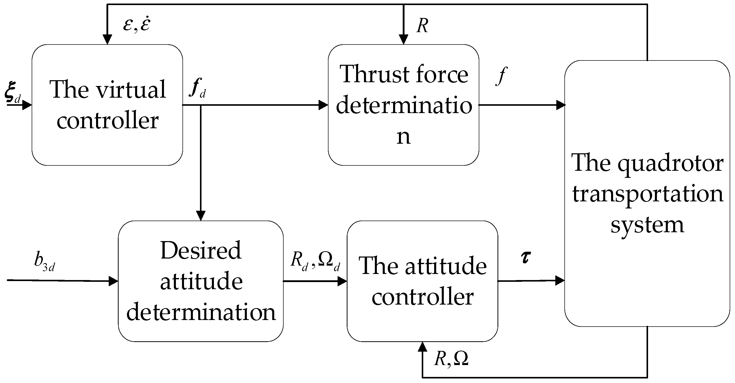
This section provides a detailed design process for the controller. The structure of the overall control scheme is shown in Figure 2.

The control objectives of this paper are the quadrotor position tracking and the elimination of the payload swing given in (16). According to $\dot{h}$ in (56)–(58), $h$ is generated by the following equation:

$$h=-k_{\lambda }{[S_1{C}_2, S_2, 1-C_1{C}_2]}^T$$

(66)

Furthermore, based on (45), ${\mathit{\chi }}_p(t)$ can be written as:

$${\mathit{\chi }}_p=\mathit{\xi }-k_{\lambda }{[S_1{C}_2,{ \mathrm{S}}_2, 1-{\mathrm{C}}_1{\mathrm{C}}_2]}^T$$

(67)

According to (67), the control objective (16) is equivalent to

$${\mathit{\chi }}_p\to {\mathit{\xi }}_d$$

(68)

Therefore, the payload positioning error $\mathit{\upsilon }(t)\in {\mathbb{R}}^3$ is defined as follows:

$$\mathit{\upsilon }={\mathit{\chi }}_p-{\mathit{\xi }}_d=e_{\xi }+h$$

(69)

Considering Equation (65), the total energy storage function can be defined as follows:

$$E_t=E_k+{\displaystyle \frac{1}{2}}{\mathit{\upsilon }}^T{\mathit{K}}_p\mathit{\upsilon }$$

(70)

where $E_t$ is positive definite, ${\mathit{K}}_p=\mathrm{d}\mathrm{i}\mathrm{a}\mathrm{g}(k_{px}, k_{py}, k_{pz})\in {\mathbb{R}}_{+}^{3\times 3}$ denotes a diagonal positive-definite gain matrix. The time derivative of $E_t(t)$ can be calculated using (46) and (69)

$${\dot{E}}_t={\dot{\mathit{\upsilon }}}^T[f\mathit{R}{\mathit{e}}_3-(M+m)g{\mathit{e}}_3+{\mathit{K}}_p\mathit{\upsilon }]$$

(71)

Substituting (22) (23) into (71) yields

$${\dot{E}}_t={\dot{\mathit{\upsilon }}}^T[{\mathit{f}}_d+\mathbf{\Delta }-(M+m)g{\mathit{e}}_3+{\mathit{K}}_p\mathit{\upsilon }]$$

(72)

The inner and outer loop coupling terms $\mathbf{\Delta }$ in (72) have both beneficial and detrimental impacts on system performance. Therefore, to make full use of the beneficial coupling term, the definition of indicator for coupling term effects is proposed as:

$$\mathit{Q}=\mathrm{sgn}[\dot{\mathit{\upsilon }}\mathbf{\Delta }]$$

(73)

The criteria for determining whether coupling terms are harmful or beneficial are as follows:

$$\left\{\begin{array}{ll}\mathit{Q}<0,\hfill & \mathrm{c}\mathrm{o}\mathrm{u}\mathrm{p}\mathrm{l}\mathrm{i}\mathrm{n}\mathrm{g} \mathrm{t}\mathrm{e}\mathrm{r}\mathrm{m} \mathrm{i}\mathrm{s} \mathrm{b}\mathrm{e}\mathrm{n}\mathrm{e}\mathrm{f}\mathrm{i}\mathrm{c}\mathrm{i}\mathrm{a}\mathrm{l}\hfill \\ \mathit{Q}=0,\hfill & \mathrm{c}\mathrm{o}\mathrm{u}\mathrm{p}\mathrm{l}\mathrm{i}\mathrm{n}\mathrm{g} \mathrm{t}\mathrm{e}\mathrm{r}\mathrm{m} \mathrm{i}\mathrm{s} \mathrm{n}\mathrm{i}\mathrm{l}\hfill \\ \mathit{Q}>0,\hfill & \mathrm{c}\mathrm{o}\mathrm{u}\mathrm{p}\mathrm{l}\mathrm{i}\mathrm{n}\mathrm{g} \mathrm{t}\mathrm{e}\mathrm{r}\mathrm{m} \mathrm{i}\mathrm{s} \mathrm{d}\mathrm{e}\mathrm{t}\mathrm{r}\mathrm{i}\mathrm{m}\mathrm{e}\mathrm{n}\mathrm{t}\mathrm{a}\mathrm{l}\hfill \end{array}\right.$$

(74)

Based on (72)–(74), the virtual control input ${\mathit{f}}_d$ is proposed as:

$$\begin{array}{ll}{\mathit{f}}_d& =-{\mathit{K}}_p\mathit{\upsilon }-{\mathit{K}}_d\dot{\mathit{\upsilon }}+(M+m)g{\mathit{e}}_3-\mathit{P}\\ & =-{\mathit{K}}_p({\mathit{e}}_{\mathit{\upsilon }}+\mathit{h})-{\mathit{K}}_d({\dot{\mathit{e}}}_{\mathit{\upsilon }}+\dot{\mathit{h}})+(M+m)g{\mathit{e}}_3-\mathit{P}\end{array}$$

(75)

where ${\mathit{K}}_d=diag(k_{dx},k_{dy},k_{dz})\in {\mathbb{R}}^{3\times 3}$ denotes a positive definite diagonal matrix, $\mathit{P}$ is defined as follows:

$$\mathit{P}=\left\{\begin{array}{c}0, \mathit{Q}\le 0\\ \mathbf{\Delta }, \mathit{Q}>0\end{array}\right.$$

(76)

The thrust $f(t)$ can be synthesized from the virtual force ${\mathit{f}}_d$ of the outer loop as follows:

$$f={\mathit{f}}_d^T\mathit{R}{\mathit{e}}_3={(-{\mathit{K}}_p\mathit{\upsilon }-{\mathit{K}}_d\dot{\mathit{\upsilon }}+(M+m)g{\mathit{e}}_3)}^T\mathit{R}{\mathit{e}}_3$$

(77)

To determine the desired attitude, the desired attitude axis vector must be calculated using the following formula

$${\mathit{b}}_{3d}={\mathit{R}}_d{\mathit{e}}_3={\displaystyle \frac{{\mathit{f}}_d}{‖{\mathit{f}}_d‖}}={\displaystyle \frac{-{\mathit{K}}_p\mathit{\upsilon }-{\mathit{K}}_d\dot{\mathit{\upsilon }}+(M+m)g{\mathit{e}}_3}{‖-{\mathit{K}}_p\mathit{\upsilon }-{\mathit{K}}_d\dot{\mathit{\upsilon }}+(M+m)g{\mathit{e}}_3‖}}$$

(78)

Therefore, the controller settings for the inner loop attitude are as follows:

$$\begin{array}{ll}\mathit{\tau }=& -{\mathit{K}}_R{\mathit{e}}_R-{\mathit{K}}_{\omega }{\mathit{e}}_{\omega }+sk(\mathit{\omega })\mathit{J}\mathit{\omega }\\ & -\mathit{J}(sk(\mathit{\omega }){\mathit{R}}^T{\mathit{R}}_d{\mathit{\omega }}_d-{\mathit{R}}^T{\mathit{R}}_d{\dot{\mathit{\omega }}}_d)\end{array}$$

(79)

where ${\mathit{K}}_R\in \mathbb{R}$ is positive constants of attitude, ${\mathit{K}}_{\omega }\in \mathbb{R}$ is positive constants of angular velocity, and the desired angular velocity ${\mathit{\omega }}_d$ can be calculated by

$${\mathit{\omega }}_d=\mathrm{v}\mathrm{e}\mathrm{x}({\mathit{R}}_d^T{\dot{\mathit{R}}}_d)$$

(80)

As shown in [35], the moment input (79) guarantees that the zero equilibrium of ${\mathit{e}}_R$ and ${\mathit{e}}_{\omega }$ is exponentially stable.

Lemma 1. 

Under the action of the virtual control input (75), the error (18) of the system asymptotically converges to zero such that

$$\underset{t\to \infty }{\lim }{[{\mathit{e}}_{\xi }^T,{\dot{\mathit{e}}}_{\xi }^T,{\mathbf{\Theta }}^T,{\dot{\mathbf{\Theta }}}^T]}^T=[0_{3\times 1}^T,0_{3\times 1}^T,0_{2\times 1}^T,0_{2\times 1}^T]$$

(81)

Proof of Lemma 1. 

Substituting (75) into (72), we can obtain:

$${\dot{E}}_t={\dot{\mathit{\upsilon }}}^T[-{\mathit{K}}_d\dot{\mathit{\upsilon }}+\mathbf{\Delta }-\mathit{P}]$$

(82)

where ${\dot{E}}_t$ should be discussed separately depending on the value of $\mathit{Q}$.

Case 1: If $\mathit{Q}>0$, it leads to

$${\dot{E}}_t=-{\dot{\mathit{\upsilon }}}^T{\mathit{K}}_d\dot{\mathit{\upsilon }}$$

(83)

The positive definite function $E_t(t)$ defined in (70) is selected as the Lyapunov candidate function $V(t)=E_t(t)$, and the time derivative of it is as follows:

$$\dot{V}=-{\dot{\mathit{\upsilon }}}^T{\mathit{K}}_d\dot{\mathit{\upsilon }}\le 0$$

(84)

Therefore, the equilibrium point of the closed-loop system is stable in the sense of Lyapunov, which can be expressed as follows by combining (69) and (75)

$$\mathit{\upsilon }, \dot{\mathit{q}}, \dot{\mathit{\xi }}, {\dot{\mathit{e}}}_{\mathit{\xi }}, \dot{x}, \dot{y}, \dot{z}, \dot{\mathbf{\Theta }}, {\dot{\theta }}_1, {\dot{\theta }}_2\in L_{\infty }$$

(85)

Combining (65) with (70) has

$${\mathit{e}}_{\mathit{\xi }}, \mathit{\xi }, \dot{\mathit{\upsilon }}, {\mathit{f}}_d\in L_{\infty }$$

(86)

Next, the signal convergence of the closed-loop system is proved, and the invariant set is defined as:

$$\Phi =\{(e_x,e_y,e_z,{\dot{e}}_x,{\dot{e}}_y,{\dot{e}}_z,{\theta }_1,{\theta }_2,{\dot{\theta }}_1,{\dot{\theta }}_2,)|\dot{V}\left(t\right)=0\}$$

(87)

Let $\Gamma$ be the largest invariant set in $\Phi$, which can be deduced from equation (84), in the invariant set $\Gamma$

$$\begin{array}{l}\dot{\mathit{\upsilon }}={\dot{\mathit{e}}}_{\mathit{\upsilon }}+\dot{\mathit{h}}={\dot{\mathit{\chi }}}_p={\mathbf{0}}_{3\times 1}\Rightarrow \\ \mathit{\upsilon }={\mathit{e}}_{\mathit{\upsilon }}+\mathit{h}={\mathit{\alpha }}_{\mathit{\upsilon }}, \ddot{\mathit{\upsilon }}={\ddot{\mathit{e}}}_{\mathit{\xi }}+\ddot{\mathit{h}}={\ddot{\mathit{\chi }}}_p={\mathbf{0}}_{3\times 1}\end{array}$$

(88)

where ${\mathit{\alpha }}_{\upsilon }={[{\alpha }_{\upsilon x},{\alpha }_{\upsilon y},{\alpha }_{\upsilon z}]}^T$ is the undetermined constant vector, and then, from (75), we can obtain:

$${\mathit{f}}_d=-{\mathit{K}}_p{\mathit{\alpha }}_{\mathit{\upsilon }}+(M+m)g{\mathit{e}}_3$$

(89)

Then, we need to prove that ${\mathit{\alpha }}_{\mathit{\upsilon }}={\mathbf{0}}_{3\times 1}$ in the maximal invariant set $\Gamma$. Taking the second-order time derivative on both sides of Equation (67), and substituting Equation (88), we can obtain

$$\ddot{x}-k_{\lambda }({\ddot{\theta }}_1{C}_1{C}_2-{\ddot{\theta }}_2{S}_1{S}_2-{\dot{\theta }}_1^2{S}_1{C}_2-{\dot{\theta }}_2^2{S}_1{C}_2-2{\dot{\theta }}_1{\dot{\theta }}_2{S}_1{S}_2)=0$$

(90)

$$\ddot{y}-k_{\lambda }({\ddot{\theta }}_2{C}_2-{\dot{\theta }}_2^2{S}_2)=0$$

(91)

$$\ddot{z}-k_{\lambda }({\ddot{\theta }}_1{S}_1{C}_2-{\ddot{\theta }}_2{C}_1{S}_2-{\dot{\theta }}_1^2{C}_1{C}_2+{\dot{\theta }}_2^2{C}_1{C}_2-2{\dot{\theta }}_1{\dot{\theta }}_2{S}_1{S}_2)=0$$

(92)

Substituting (89) into (37)–(39) becomes

$$(M+m)\ddot{x}+ml({\ddot{\theta }}_1{C}_1{C}_2-{\ddot{\theta }}_2{S}_1{S}_2-{\dot{\theta }}_1^2{S}_1{C}_2-{\dot{\theta }}_2^2{S}_1{C}_2-2{\dot{\theta }}_1{\dot{\theta }}_2{C}_1{S}_2)=-k_{px}{\alpha }_{\epsilon x}$$

(93)

$$(M+m)\ddot{y}+ml({\ddot{\theta }}_2{C}_2-{\dot{\theta }}_2^2{S}_2)=-k_{py}{\alpha }_{\epsilon y}$$

(94)

$$(M+m)\ddot{z}+ml({\ddot{\theta }}_1{S}_1{C}_2+{\ddot{\theta }}_2{C}_1{S}_2+{\dot{\theta }}_1^2{C}_1{C}_2+{\dot{\theta }}_2^2{C}_1{C}_2-2{\dot{\theta }}_1{\dot{\theta }}_2{S}_1{S}_2)=-k_{pz}{\alpha }_{\epsilon z}$$

(95)

According to (90)–(95), the following can be obtained:

$$\ddot{x}=-{\displaystyle \frac{k_{\lambda }{k}_{px}{\alpha }_{\mathit{\upsilon }x}}{k_{\lambda }(M+m)+ml}}$$

(96)

$$\ddot{y}=-{\displaystyle \frac{k_{\lambda }{k}_{py}{\alpha }_{\mathit{\upsilon }y}}{k_{\lambda }(M+m)+ml}}$$

(97)

$$\ddot{z}=-{\displaystyle \frac{k_{\lambda }{k}_{pz}{\alpha }_{\mathit{\upsilon }z}}{k_{\lambda }(M+m)+ml}}$$

(98)

Taking ${\alpha }_{\mathit{\upsilon }x}$ as an example. If ${\alpha }_{\mathit{\upsilon }x}\ne 0$, it can be concluded that when $t\to \infty$, $\dot{x}\to \infty$ is obviously inconsistent with the conclusion $\dot{x}\in L_{\infty }$ in (85). Therefore, this hypothesis is not valid. Through similar analysis, we can see that in the set $\Gamma$

$${\mathit{\alpha }}_{\mathit{\upsilon }}={\mathbf{0}}_{3\times 1}\Rightarrow \mathit{\upsilon }={\mathbf{0}}_{3\times 1}$$

(99)

$${\mathit{f}}_d=(M+m)g{\mathit{e}}_3$$

(100)

$$\ddot{\mathit{\xi }}={\mathbf{0}}_{3\times 1}\Rightarrow \dot{\mathit{\xi }}={\mathit{\alpha }}_{\dot{\mathit{\xi }}}$$

(101)

where ${\mathit{\alpha }}_{e\mathit{\xi }}\in {\mathbb{R}}^3$ is the undetermined constant vector. Similarly, one can conclude that in the set $\Gamma$

$$\dot{\mathit{\xi }}={\mathbf{0}}_{3\times 1}\Rightarrow {\dot{\mathit{e}}}_{\mathit{\xi }}={\mathbf{0}}_{3\times 1}, {\mathit{e}}_{\mathit{\xi }}={\mathit{\alpha }}_{e\mathit{\xi }}$$

(102)

where ${\mathit{\alpha }}_{e\mathit{\xi }}\in {\mathbb{R}}^3$ is the undetermined constant vector. Therefore, $\dot{\mathit{h}}={\mathbf{0}}_{3\times 1}$ can be deduced from (88) and (102). And the following conclusions can be obtained from (56)–(58)

$${\dot{\theta }}_1{C}_1{C}_2-{\dot{\theta }}_2{S}_1{S}_2=0$$

(103)

$${\dot{\theta }}_2{C}_2=0$$

(104)

$${\dot{\theta }}_1{S}_1{C}_2+{\dot{\theta }}_2{C}_1{S}_2=0$$

(105)

Considering the payload’s swing angle $-{\displaystyle \frac{\pi }{2}}<{\theta }_x, {\theta }_y<{\displaystyle \frac{\pi }{2}}$ in the actual situation, it can be proved that

$${\dot{\theta }}_1=0, {\dot{\theta }}_2=0\Rightarrow {\ddot{\theta }}_1=0, {\ddot{\theta }}_2=0$$

(106)

On this basis, using (40)–(41), (66), (99)–(101) (106), and (88) the following can be obtained:

$${\theta }_x=0, {\theta }_y=0\Rightarrow \mathit{h}={\mathbf{0}}_{3\times 1}\Rightarrow {\mathit{e}}_{\mathit{\xi }}={\mathbf{0}}_{3\times 1}, \mathit{\xi }={\mathit{\xi }}_d$$

(107)

Combining (99)–(101), (106), and (107), the maximum invariant set contains only the equilibrium point

$${[{\mathit{e}}_{\mathit{\xi }}^T,{\dot{\mathit{e}}}_{\mathit{\xi }}^T,{\mathit{\theta }}^T,{\dot{\mathit{\theta }}}^T]}^T={[{\mathbf{0}}_{3\times 1}^T,{\mathbf{0}}_{3\times 1}^T,{\mathbf{0}}_{2\times 1}^T,{\mathbf{0}}_{2\times 1}^T]}^T$$

(108)

The above conclusion is proved by the LaSalle invariance principle.

Case 2: If $\mathit{Q}\le 0$, one can obtain

$${\dot{E}}_t={\dot{\mathit{\upsilon }}}^T[-{\mathit{K}}_d\dot{\mathit{\upsilon }}+\mathbf{\Delta }]$$

(109)

When the coupling term $\mathbf{\Delta }$ is ignored, the stability proof process is the same as that of Case 1, so the stability of the whole system can be proved as long as the coupling term meets the growth restriction condition. □

Lemma 2. 

There exists a normal number $d_{\mathbf{\Delta }}\in {\mathbb{R}}_{+}$ and a differentiable $\kappa -class$ function $\gamma (·)$ at the point ${[{\mathit{e}}_R^T,{\mathit{e}}_{\omega }^T]}^T={\mathbf{0}}_{6\times 1}$ such that the coupling term $\mathit{\eta }$ satisfies the following growth constraints:

$$‖\mathit{\beta }‖\le \gamma ({\mathit{e}}_R)‖\mathit{e}‖, if‖\mathit{e}‖\ge d_{\mathbf{\Delta }}$$

(110)

Proof of Lemma 2. 

To prove the lemma, the boundedness of the signal $\mathit{h}$, $\dot{\mathit{h}}$ should be first analyzed, and the following conclusions are drawn from (66)

$$\begin{array}{ll}‖\mathit{h}‖& =k_{\lambda }\sqrt{{(S_1{C}_2)}^2+{(S_2)}^2+{(1-C_1{C}_2)}^2}\\ & \le k_{\lambda }\sqrt{2-2C_1{C}_2}\\ & \le 2k_{\lambda }\end{array}$$

(111)

From (56)–(58), $‖\dot{\mathit{h}}‖$ can be scaled as follows:

$$\begin{array}{ll}‖\dot{\mathit{h}}‖& =k_{\lambda }\sqrt{\begin{array}{l}{({\dot{\theta }}_1{C}_1{C}_2-{\dot{\theta }}_2{S}_1{S}_2)}^2+{({\dot{\theta }}_2{C}_2)}^2\\ +{({\dot{\theta }}_1{S}_1{C}_2+{\dot{\theta }}_2{C}_1{S}_2)}^2\end{array}}\\ & \le k_{\lambda }\sqrt{{({\dot{\theta }}_1{C}_2)}^2+{({\dot{\theta }}_2{S}_2)}^2+{({\dot{\theta }}_2{C}_2)}^2}\\ & \le k_{\lambda }\sqrt{{\dot{\theta }}_1^2+{\dot{\theta }}_2^2}\\ & =k_{\lambda }‖\dot{\mathbf{\Theta }}‖\end{array}$$

(112)

Let ${\lambda }_p$ and ${\lambda }_d$ represent the maximum eigenvalues of control gain ${\mathit{K}}_p$ and ${\mathit{K}}_d$ respectively. According to (111) and (112), it is not difficult to obtain

$$\begin{array}{ll}‖{\mathit{f}}_d‖& =‖-{\mathit{K}}_p\mathit{\upsilon }-{\mathit{K}}_d\dot{\mathit{\upsilon }}+(M+m)g{\mathit{e}}_3‖\\ & \le \max ({\lambda }_p,{\lambda }_d)(‖\mathit{\upsilon }‖+‖\dot{\mathit{\upsilon }}‖)+(M+m)g\\ & \le \max ({\lambda }_p,{\lambda }_d)(‖{\mathit{e}}_{\mathit{\xi }}‖+‖\mathit{h}‖+‖{\dot{\mathit{e}}}_{\mathit{\xi }}‖+‖\dot{\mathit{h}}‖)\\ & \hspace{1em}+(M+m)g\\ & \le 2\max ({\lambda }_p,{\lambda }_d)\cdot \max (1,k_{\lambda })‖\mathit{e}‖\\ & \hspace{1em}+(M+m)g+2k_{\lambda }\max ({\lambda }_p,{\lambda }_d)\end{array}$$

(113)

Defining the following parameters:

$$\begin{array}{l}{c}_f=4\max ({\lambda }_p,{\lambda }_d)\cdot \max (1,k_{\lambda })\\ d_f={\displaystyle \frac{(M+m)g+2k_{\lambda }\max ({\lambda }_p,{\lambda }_d)}{2\max ({\lambda }_p,{\lambda }_d)\cdot \max (1,k_{\lambda })}}\end{array}$$

(114)

There is a normal number $d_f,c_f\in {\mathbb{R}}_{+}$ such that the virtual control input vector ${\mathit{f}}_d(t)$ satisfies:

$$‖{\mathit{f}}_d(\mathit{e})‖=\left\{\begin{array}{c}{c}_f‖\mathit{e}‖, \mathrm{i}\mathrm{f}‖\mathit{e}‖\ge d_f\\ c_f{d}_f, \mathrm{i}\mathrm{f}‖\mathit{e}‖<d_f\end{array}\right.$$

(115)

Combining (22) with (77) and (78), the following can be obtained:

$$‖\mathbf{\Delta }‖=‖{\mathit{f}}_d‖‖({\mathit{e}}_3^T{\mathit{R}}_d^T\mathit{R}{\mathit{e}}_3)\mathit{R}{\mathit{e}}_3-{\mathit{R}}_d{\mathit{e}}_3‖$$

(116)

where $‖({\mathit{e}}_3^T{\mathit{R}}_d^T\mathit{R}{\mathit{e}}_3)\mathit{R}{\mathit{e}}_3-{\mathit{R}}_d{\mathit{e}}_3‖$ represents the sine value of the angle between the vector $\mathit{R}{\mathit{e}}_3$ and the vector ${\mathit{R}}_d{\mathit{e}}_3$, $‖{\mathit{e}}_R‖$ represents the angle between the rotation matrix $\mathit{R}$ and the characteristic axis of ${\mathit{R}}_d$. Therefore, considering (115), we have

$$\begin{array}{ll}‖\mathbf{\Delta }‖& \le ‖{\mathit{f}}_d‖‖{\mathit{e}}_R‖\\ & \le k_f‖\mathit{e}‖‖{\mathit{e}}_R‖,\hspace{1em}\mathrm{i}\mathrm{f}‖\mathit{e}‖\ge d_f\end{array}$$

(117)

Combining $\mathit{\eta }$, ${\mathbf{\Delta }}_u$ and (117), the following inequation can be obtained:

$$\begin{array}{ll}‖\mathit{\eta }‖& \le {‖{\mathbf{\prod }}_{01}{\mathit{M}}_c^{-1}‖}_F‖{\mathbf{\Delta }}_u‖\\ & ={‖{\mathbf{\prod }}_{01}{\mathit{M}}_c^{-1}‖}_F‖\mathbf{\Delta }‖\\ & \le c_f{‖{\mathbf{\prod }}_{01}{\mathit{M}}_c^{-1}‖}_F‖{\mathit{e}}_R‖‖\mathit{e}‖,\hspace{1em}\mathrm{i}\mathrm{f}‖\mathit{e}‖\ge d_f\end{array}$$

(118)

where ${‖\mathbf{·}‖}_F$ represents the Frobenius norm of the matrix. Select

$$\begin{array}{l}\gamma ({\mathit{e}}_R)=c_f{‖{\mathbf{\prod }}_{01}{\mathit{M}}_c^{-1}‖}_F‖{\mathit{e}}_R‖\\ d_{\mathbf{\Delta }}=d_f\end{array}$$

(119)

Therefore, lemma1 and lemma 2 are proved. □

Theorem 1. 

The thrust input (75) and torque input (79) can enforce the quadrotor to track the desired position, and ensure the elimination of payload swing angle, i.e.,

$$\begin{array}{l}\underset{t\to \infty }{\lim }{[{\mathit{\xi }}^T,{\dot{\mathit{\xi }}}^T,{\theta }_1,{\theta }_2,{\dot{\theta }}_1,{\dot{\theta }}_2,{\mathit{e}}_R^T,{\mathit{e}}_{\omega }^T]}^T\\ ={[{\mathit{\xi }}_d^T,{\mathbf{0}}_{3\times 1}^T,0,0,0,0,{\mathbf{0}}_{3\times 1}^T,{\mathbf{0}}_{3\times 1}^T]}^T\end{array}$$

(120)

Proof of Theorem 1. 

According to Lemma 1 and Lemma 2 and the stability of inner loop tracking, it can be proved that the equilibrium point is asymptotically stable. □

5. Simulation Results and Analysis

This section includes four sets of simulation experiments designed to validate the superiority of the proposed control scheme. The first set is compared with the energy-coupling control method [32] to verify the better performance of the proposed method, and the second group tests its robustness against external disturbance and parametric uncertainty.

The body mass, payload mass, gravity acceleration, rope length, and moment of inertia are set as follows:

$$\begin{array}{l}M=0.645 \mathrm{k}\mathrm{g}, m=0.075 \mathrm{k}\mathrm{g}, g=9.8 \mathrm{k}\mathrm{g}\cdot \mathrm{m}/{\mathrm{s}}^2,\\ l=0.535 \mathrm{m}, \mathit{J}=\mathrm{d}\mathrm{i}\mathrm{a}\mathrm{g}(0.010,0.010,0.012) \mathrm{k}\mathrm{g}\cdot {\mathrm{m}}^2\end{array}$$

The inner loop control gains of the two controllers are uniformly chosen:

$${\mathit{K}}_R=\mathrm{d}\mathrm{i}\mathrm{a}\mathrm{g}(5.3, 5.3, 6.2)$$

$${\mathit{K}}_{\omega }=\mathrm{d}\mathrm{i}\mathrm{a}\mathrm{g}(0.5, 0.5, 1.0)$$

For the energy-coupling control method, the control gains are selected as:

$${\mathit{K}}_P=\mathrm{d}\mathrm{i}\mathrm{a}\mathrm{g}(2.7, 1.8, 7.0)$$

$${\mathit{K}}_d=\mathrm{d}\mathrm{i}\mathrm{a}\mathrm{g}(4.6, 3.1, 10)$$

$${\mathit{K}}_{\lambda }=1.8$$

The control gains for the proposed control design are tuned as follows:

$${\mathit{K}}_d=\mathrm{d}\mathrm{i}\mathrm{a}\mathrm{g}(5.1, 2.8, 10)$$

$${\mathit{K}}_d=\mathrm{d}\mathrm{i}\mathrm{a}\mathrm{g}(5.1, 2.8, 10)$$

$${\mathit{K}}_{\lambda }=3.5$$

• Simulation Test 1: Control Performance

To adjust the quadrotor’s position along the $x$, $y$, and $z$ axes, set the following parameters:

$$\mathit{\xi }(0)={[1.0, 1.3, 1.5]}^T\to {\mathit{\xi }}_d={[0.5, 0.3, 1.0]}^T$$

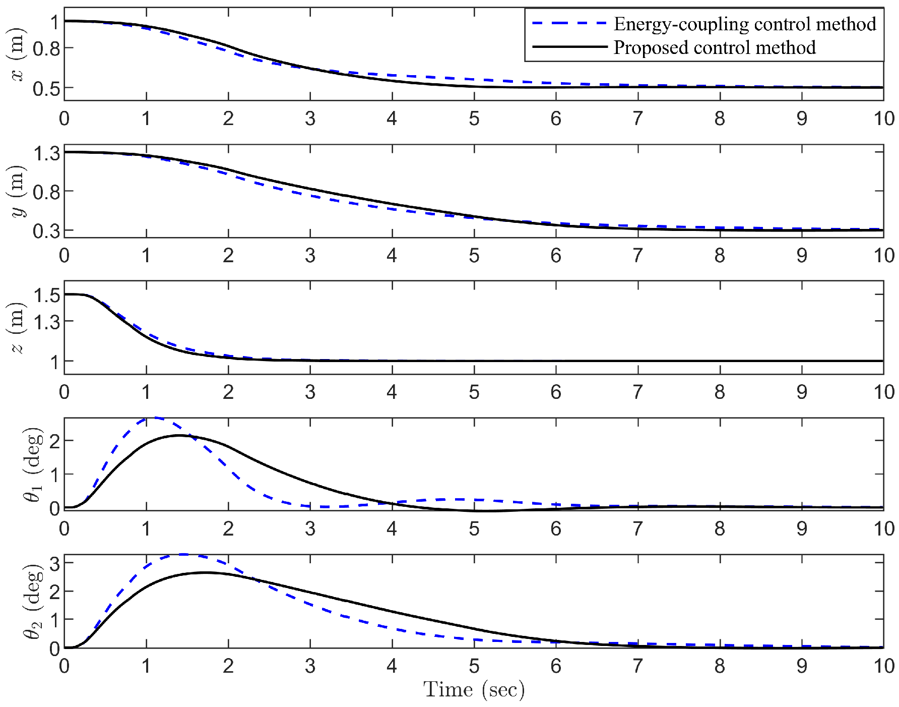
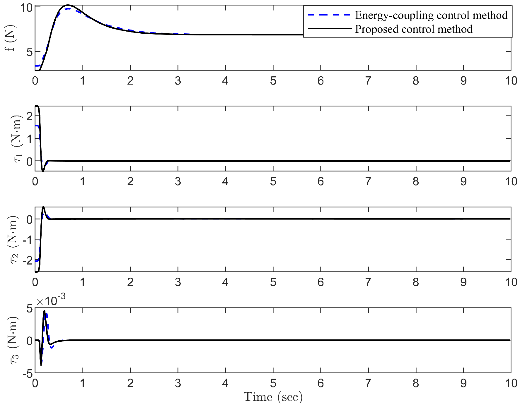
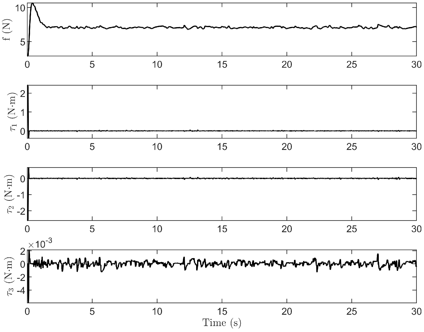
Figure 3 shows that both control methods move the quadrotor from the initial position to the desired position along similar trajectories. Figure 4 shows the torque and input on each axis. However, the proposed control method suppresses the swing angle more effectively.

Table 1. Quantitative data for simulation test 1.

Simulation Test 1	Max		Mean		RMS
	${\mathit{\theta }}_1$	${\mathit{\theta }}_2$	${\mathit{\theta }}_1$	${\mathit{\theta }}_2$	${\mathit{\theta }}_1$	${\mathit{\theta }}_2$
Proposed controller	2.14°	2.64°	0.43°	0.86°	0.84°	1.29°
Energy-coupling controller	2.67°	3.30°	0.44°	0.88°	0.87°	1.38°

shows that the maximum payload swing angles for the energy-coupling method are 2.67° and 3.30°, while the proposed control method achieves 2.14° and 2.64° for its maximum swing angles. In comparison, the proposed control method achieves a 20% improvement in suppressing the swing angle. Furthermore, the mean and RMS values in Table 1 further indicate that the proposed control method exhibits higher stability. Furthermore, Figure 5 shows that the proposed control method leads to smaller attitude angles and improved rotational characteristics.

• Simulation Test 2: Robustness Verification Experiment

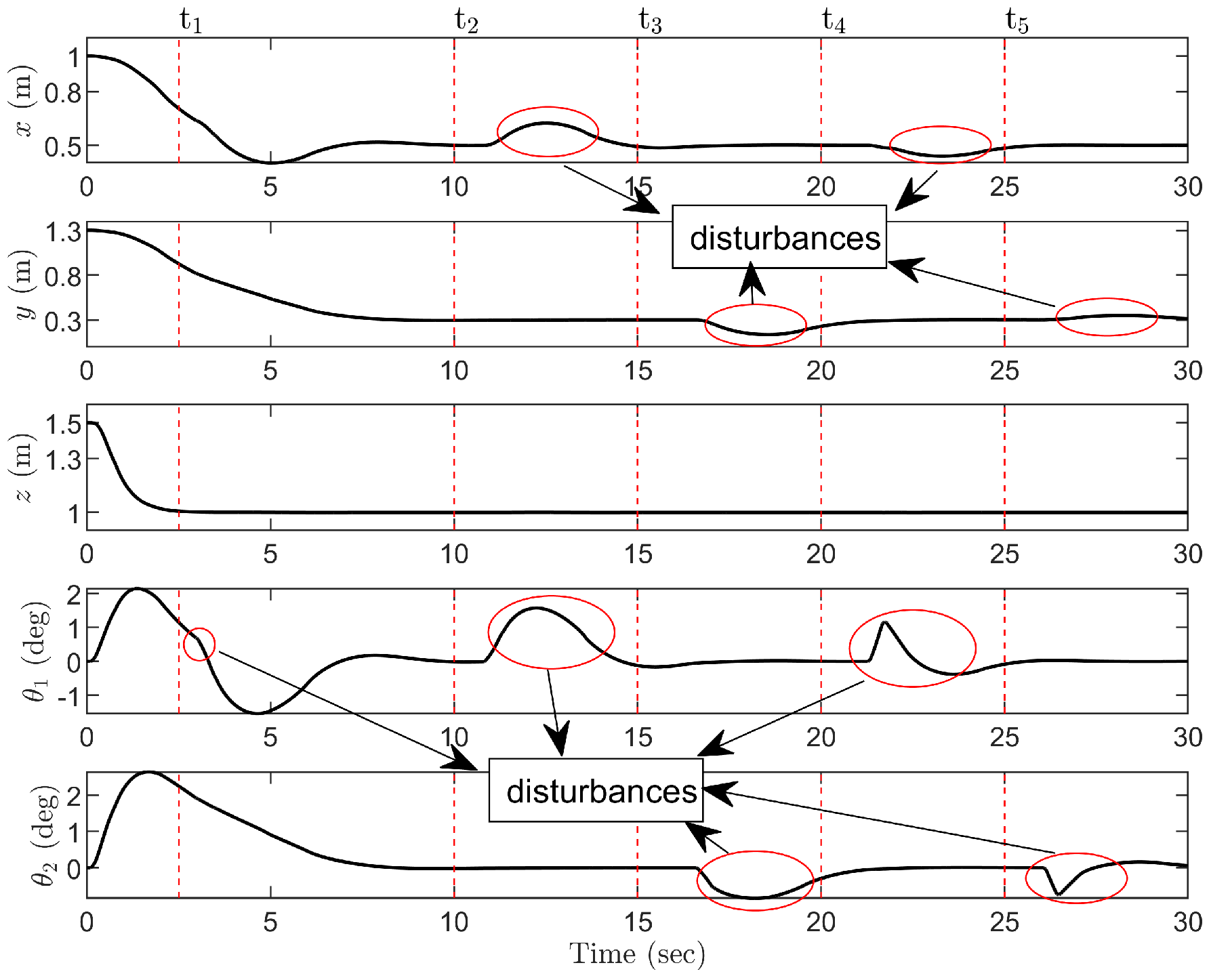
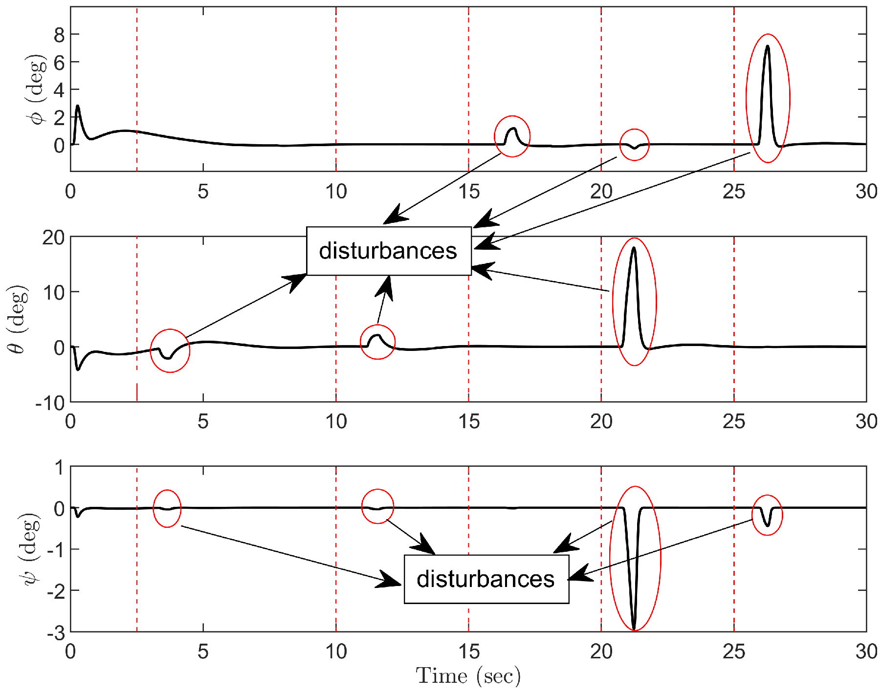
Next, two groups of disturbance-rejection simulation tests are presented. The first group gives external disturbance in different directions to test the robustness of the system under the condition of using the parameters of Simulation Test 1. The second group changes the rope length and payload mass. New initial and desired positions are selected to test the effects of internal disturbances on the system.

In the first robustness simulation tests, pulse signals are utilized to simulate external disturbances affecting the system, applied in various directions to both the quadrotor and the payload. The control performance is shown in Figure 6, Figure 7 and Figure 8. In the process of quadrotor transportation, even if the payload is affected by external disturbance at $t_1$, the proposed control method can still ensure the accurate arrival of the quadrotor to the target position and the effective suppression of the payload swing. When the external disturbance is applied at $t_2$ and $t_3$ from different directions of the payload, the QTS can still restore quickly to the equilibrium state. Furthermore, when the position of the quadrotor is offset by the external disturbance at $t_4$ and $t_5$, the proposed algorithm can still ensure the system stability.

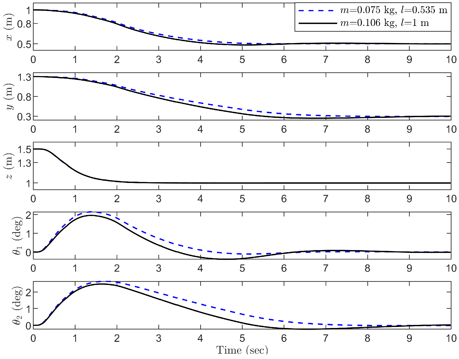
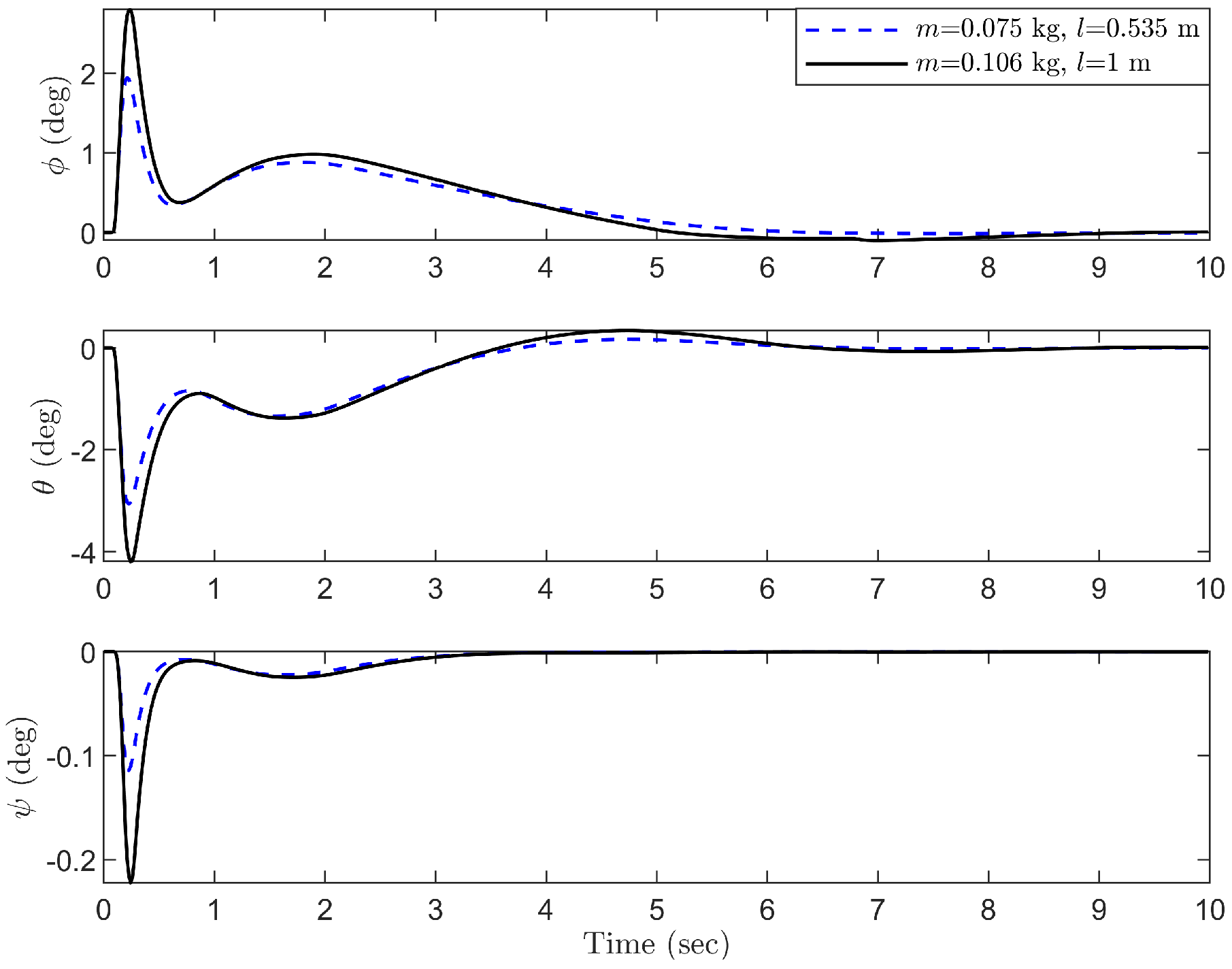
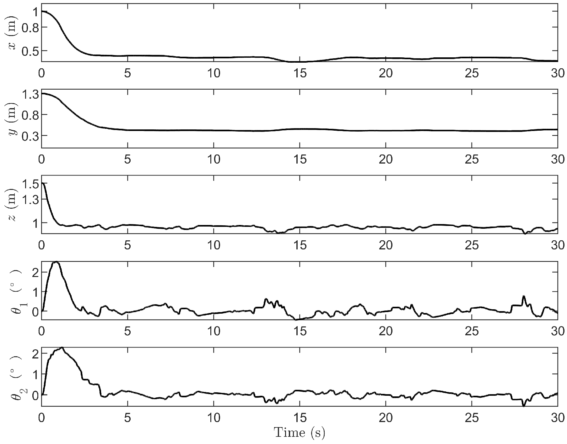
To assess the robustness of the proposed control scheme against internal disturbances such as uncertain rope length and payload mass, two scenarios are considered. (1) $l=1 \mathrm{m}$, $m=0.106 \mathrm{k}\mathrm{g}$; (2) $l=0.535 \mathrm{m}$, $m=0.075 \mathrm{k}\mathrm{g}$ in the second simulation test. The control performance is shown in Figure 9, Figure 10 and Figure 11. As can be seen from these curves, the quadrotor can still reach the desired position quickly and stably under the varying rope length and payload mass. The payload swing angle can be kept within 3 degrees. At the same time, the attitude of the quadrotor body also remained within the normal range.

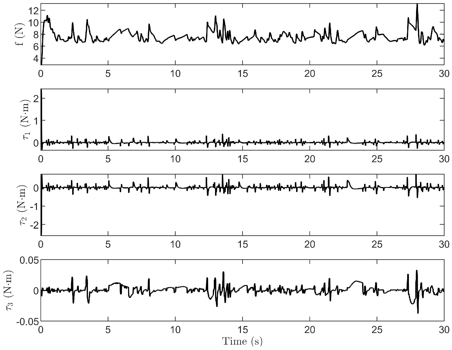
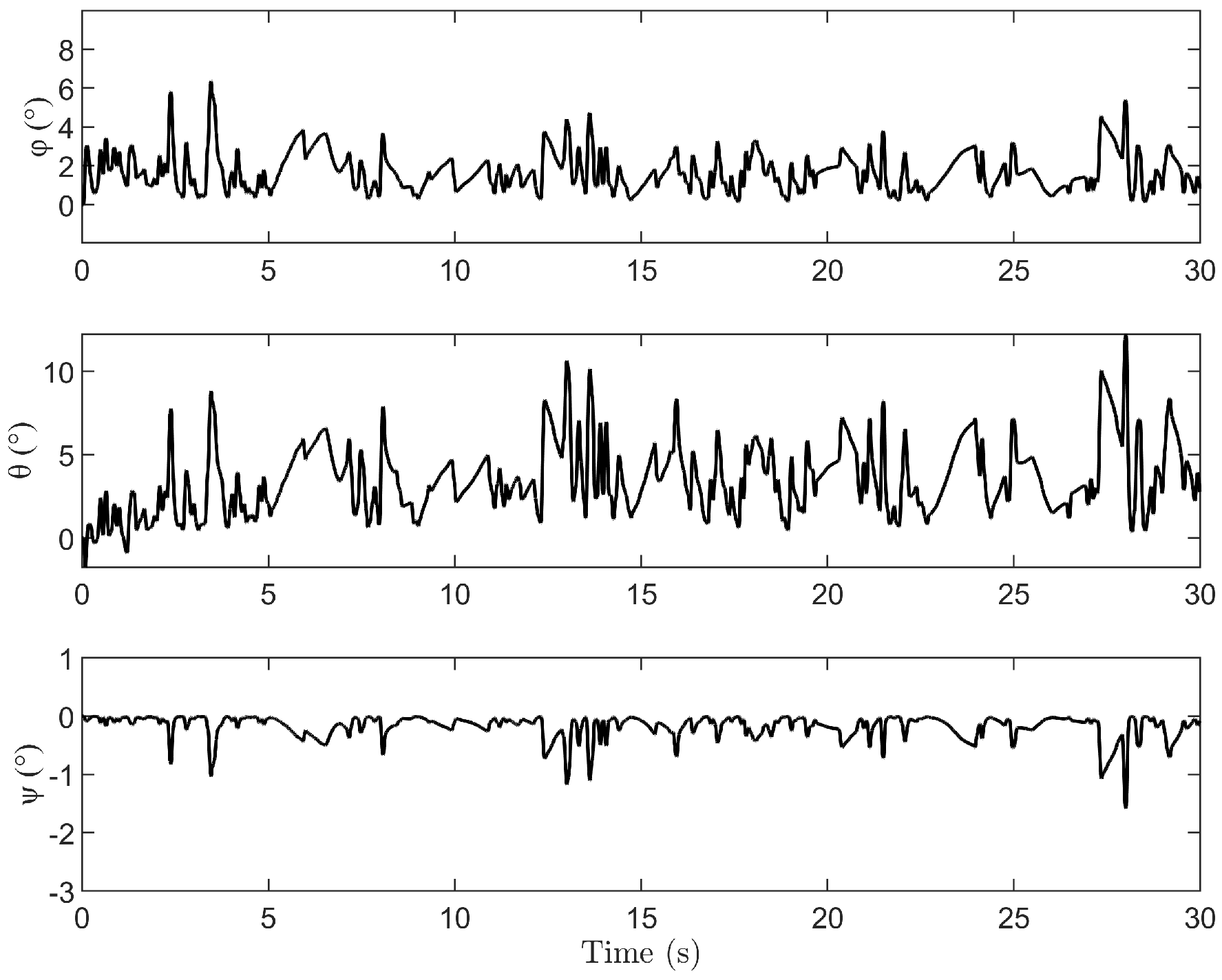
• Simulation Test 3: Robustness to wind gust effect.

Figure 12, Figure 13 and Figure 14 show the simulation results of the wind gust effect. Despite the influence of wind gusts, the system maintains accurate positioning at the desired location. Additionally, the maximum payload swing angle remains within 3 degrees, and after reaching the desired position, the payload swing angle stays within 1 degree. This demonstrates that the system retains strong robustness against irregular wind gusts.

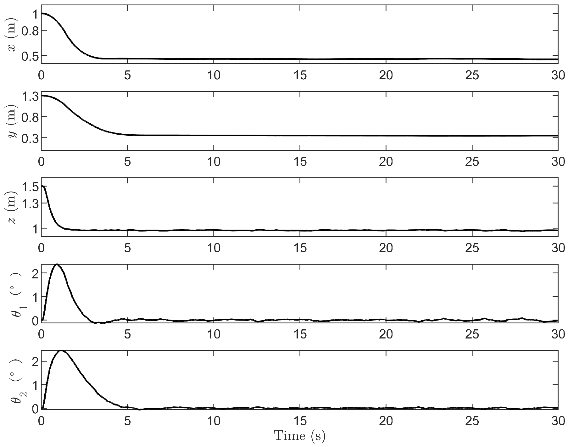
• Simulation Test 4: Robustness to ground reflection effect

Figure 15, Figure 16 and Figure 17 illustrate the state of the rotorcraft lifting system considering the ground reflection effect. The system maintains accurate positioning throughout the movement, and the maximum payload swing angle remains within 3 degrees. Additionally, after the system reaches the desired position, the load swing angle demonstrates strong robustness.

6. Conclusions

Beneficial coupling terms between the inner and outer loops are assessed to enhance the system’s transient performance. A new energy-coupling-based control method is proposed to realize the quadrotor positioning and the payload swing elimination simultaneously. Firstly, a generalized payload is introduced, and then a new passive characteristic of the QTS is proposed. Secondly, a judgment function is designed to determine whether the coupling is harmful or beneficial, and the beneficial coupling is reserved to improve the transient characteristics of the system. By constructing a new energy storage function, we develop a novel control signal of the outer loop subsystem, which can guarantee the tracking performance of the quadrotor transport system with the inner-loop attitude tracking controller. Various simulation results are performed in this paper to verify the feasibility and effectiveness. The proposed method not only has better positioning tracking and swing elimination ability but also significantly improves attitude control performance.

References

1. Derrouaoui, S.H.; Bouzid, Y.; Guiatni, M. Adaptive Integral Backstepping Control of a Reconfigurable Quadrotor with Variable Parameters’ Estimation. Proc. Inst. Mech. Eng. Part J. Syst. Control Eng. 2022, 236, 1294–1309. [Google Scholar] [CrossRef]
2. Fu, S.; Saeidi, H.; Huang, J.; Wang, Y.; Wagner, J. Customizable Unmanned Aerial Vehicle Haptic Feedback Interface: Theory and Test. J. Guid. Control Dyn. 2018, 41, 2581–2587. [Google Scholar] [CrossRef]
3. Xian, B.; Wang, S.; Yang, S. An Online Trajectory Planning Approach for a Quadrotor UAV with a Slung Payload. IEEE Trans. Ind. Electron. 2020, 67, 6669–6678. [Google Scholar] [CrossRef]
4. Hou, Y.; Chen, D.; Yang, S. Adaptive Robust Trajectory Tracking Controller for a Quadrotor UAV with Uncertain Environment Parameters Based on Backstepping Sliding Mode Method. IEEE Trans. Autom. Sci. Eng. 2023, 1–11. [Google Scholar] [CrossRef]
5. Fu, X.; He, J. Robust Adaptive Sliding Mode Control Based on Iterative Learning for Quadrotor UAV. IETE J. Res. 2023, 69, 5484–5496. [Google Scholar] [CrossRef]
6. Jo, S.; Jang, S.-A.; Choi, K. Analysis on Dynamic Characteristics and LQR Control of a Quadrotor Aircraft with Cyclic Pitch. J. Korean Soc. Aeronaut. Space Sci. 2013, 41, 217–225. [Google Scholar] [CrossRef]
7. Lee, K.; Kim, S.; Kwak, S.; You, K. Quadrotor Stabilization and Tracking Using Nonlinear Surface Sliding Mode Control and Observer. Appl. Sci. 2021, 11, 1417. [Google Scholar] [CrossRef]
8. Chen, T.; Shan, J. A Novel Cable-Suspended Quadrotor Transportation System: From Theory to Experiment. Aerosp. Sci. Technol. 2020, 104, 105974. [Google Scholar] [CrossRef]
9. Yang, S.; Han, J.; Xia, L.; Chen, Y.-H. Adaptive Robust Servo Constraint Tracking Control for an Underactuated Quadrotor UAV with Mismatched Uncertainties. ISA Trans. 2020, 106, 12–30. [Google Scholar] [CrossRef] [PubMed]
10. Cruz, P.J.; Fierro, R. Cable-Suspended Load Lifting by a Quadrotor UAV: Hybrid Model, Trajectory Generation, and Control. Auton. Robots 2017, 41, 1629–1643. [Google Scholar] [CrossRef]
11. Sreenath, K.; Michael, N.; Kumar, V. Trajectory Generation and Control of a Quadrotor with a Cable-Suspended Load—A Differentially-Flat Hybrid System. In Proceedings of the 2013 IEEE International Conference on Robotics and Automation, Karlsruhe, Germany, 6–10 May 2013; pp. 4888–4895. [Google Scholar]
12. Sierra-García, J.E.; Santos, M. Intelligent Control of an UAV with a Cable-Suspended Load Using a Neural Network Estimator. Expert Syst. Appl. 2021, 183, 115380. [Google Scholar] [CrossRef]
13. Lee, B.-Y.; Oh, H.-S.; Tahk, M.-J.; Lee, H.-I. Slung-Load Trajectory Control Using an Input-Shaping Method with Model-Following Control. Int. J. Robot. Autom. 2022, 37, 60–75. [Google Scholar]
14. Hua, H.; Fang, Y.; Zhang, X.; Qian, C. A Time-Optimal Trajectory Planning Strategy for an Aircraft with a Suspended Payload via Optimization and Learning Approaches. IEEE Trans. Control Syst. Technol. 2022, 30, 2333–2343. [Google Scholar] [CrossRef]
15. López García, M.; Martínez Carranza, J.; López García, M.; Martínez Carranza, J. A First CNN-Based Approach Towards Autonomous Flight for Object Lifting. Comput. Sist. 2020, 24, 1219–1228. [Google Scholar] [CrossRef]
16. Faust, A.; Palunko, I.; Cruz, P.; Fierro, R.; Tapia, L. Automated Aerial Suspended Cargo Delivery through Reinforcement Learning. Artif. Intell. 2017, 247, 381–398. [Google Scholar] [CrossRef]
17. Liang, X.; Zhang, Z.; Yu, H.; Wang, Y.; Fang, Y.; Han, J. Antiswing Control for Aerial Transportation of the Suspended Cargo by Dual Quadrotor UAVs. IEEE ASME Trans. Mechatron. 2022, 27, 5159–5172. [Google Scholar] [CrossRef]
18. Nicotra, M.M.; Garone, E.; Naldi, R.; Marconi, L. Nested Saturation Control of an UAV Carrying a Suspended Load. In Proceedings of the 2014 American Control Conference, Portland, OR, USA, 4–6 June 2014; pp. 3585–3590. [Google Scholar]
19. Guerrero-Sánchez, M.E.; Mercado-Ravell, D.A.; Lozano, R.; García-Beltrán, C.D. Swing-Attenuation for a Quadrotor Transporting a Cable-Suspended Payload. ISA Trans. 2017, 68, 433–449. [Google Scholar] [CrossRef] [PubMed]
20. Liang, X.; Fang, Y.; Sun, N.; Lin, H. Nonlinear Hierarchical Control for Unmanned Quadrotor Transportation Systems. IEEE Trans. Ind. Electron. 2018, 65, 3395–3405. [Google Scholar] [CrossRef]
21. Borja, P.; Cisneros, R.; Ortega, R. A Constructive Procedure for Energy Shaping of Port—Hamiltonian Systems. Automatica 2016, 72, 230–234. [Google Scholar] [CrossRef]
22. Yokoyama, K.; Takahashi, M. Dynamics-Based Nonlinear Acceleration Control with Energy Shaping for a Mobile Inverted Pendulum with a Slider Mechanism. IEEE Trans. Control Syst. Technol. 2016, 24, 40–55. [Google Scholar] [CrossRef]
23. Delgado, S.; Kotyczka, P. Energy Shaping for Position and Speed Control of a Wheeled Inverted Pendulum in Reduced Space. Automatica 2016, 74, 222–229. [Google Scholar] [CrossRef]
24. Kosucki, A.; Stawiński, Ł.; Malenta, P.; Zaczyński, J.; Skowrońska, J. Energy Consumption and Energy Efficiency Improvement of Overhead Crane’s Mechanisms. Eksploat. Niezawodn.—Maint. Reliab. 2020, 22, 323–330. [Google Scholar] [CrossRef]
25. Su, T.-S.; Wu, C.-C.; Yang, H.-R. An Analysis of Energy Consumption and Cost-Effectiveness for Overhead Crane Drive Systems by Using Fuzzy Multi-Objective Linear Programming. J. Intell. Fuzzy Syst. 2018, 35, 6241–6253. [Google Scholar] [CrossRef]
26. Fan, B.; Zhang, Y.; Sun, L.; Wang, L.; Liao, Z. Passivity and Underactuated Modeling-Based Load Energy Coupling Control for Three-Dimensional Overhead Crane Systems. Mechatronics 2023, 96, 103062. [Google Scholar] [CrossRef]
27. Peng, X.; Zhang, Z.; Zhang, A.; Yuen, K.-V. Antisaturation Backstepping Control for Quadrotor Slung Load System with Fixed-Time Prescribed Performance. IEEE Trans. Aerosp. Electron. Syst. 2024, 60, 4170–4181. [Google Scholar] [CrossRef]
28. Wang, C.; Fan, B.; Zhao, Y.; Zhang, Y.; Sun, L. Energy Coupling-Based Double-Pendulum Variable Rope Length Underactuated Control for Quadrotor UAV with Slung Load. J. Braz. Soc. Mech. Sci. Eng. 2024, 46, 592. [Google Scholar] [CrossRef]
29. Zhang, Y.; Fan, B.; Sun, L.; Huang, G.; Zhao, Y. An Enhanced Energy Coupling-Based Control Method for Quadrotor UAV Suspended Payload with Variable Rope Length. Int. J. Precis. Eng. Manuf. 2024, 25, 2321–2336. [Google Scholar] [CrossRef]
30. Zhang, Z.; Peng, X.; Zhang, A. Trajectory Tracking Control for Quadrotor Slung Load System with Unknown Load’s Linear Velocity and Cable Length. IEEE Trans. Intell. Veh. 2024, 9, 2576–2587. [Google Scholar] [CrossRef]
31. Viola, G.; Ortega, R.; Banavar, R.; Acosta, J.A.; Astolfi, A. Total Energy Shaping Control of Mechanical Systems: Simplifying the Matching Equations Via Coordinate Changes. IEEE Trans. Autom. Control 2007, 52, 1093–1099. [Google Scholar] [CrossRef]
32. Liang, X.; Fang, Y.; Sun, N.; Lin, H. A Novel Energy-Coupling-Based Hierarchical Control Approach for Unmanned Quadrotor Transportation Systems. IEEEASME Trans. Mechatron. 2019, 24, 248–259. [Google Scholar] [CrossRef]
33. Garcia, O.; Rojo-Rodriguez, E.G.; Sanchez, A.; Saucedo, D.; Munoz-Vazquez, A.J. Robust Geometric Navigation of a Quadrotor UAV on SE(3). Robotica 2020, 38, 1019–1040. [Google Scholar] [CrossRef]
34. Zhang, M.; Jing, X.; Zhang, L.; Huang, W.; Li, S. Toward a Finite-Time Energy-Saving Robust Control Method for Active Suspension Systems: Exploiting Beneficial State-Coupling, Disturbance, and Nonlinearities. IEEE Trans. Syst. Man Cybern. Syst. 2023, 53, 5885–5896. [Google Scholar] [CrossRef]
35. Lee, T.; Leok, M.; McClamroch, N.H. Geometric Tracking Control of a Quadrotor UAV on SE(3). In Proceedings of the 49th IEEE Conference on Decision and Control (CDC), Atlanta, GA, USA, 15–17 December 2010; pp. 5420–5425. [Google Scholar]
Figure 1. Quadrotor transportation system.
Actuators 14 00091 g001
Figure 2. Structure of the overall control system.
Actuators 14 00091 g002
Figure 3. And  Θ ( t )  for QTS.
Actuators 14 00091 g003
Figure 4. Control inputs  f ( t ) τ ( t ) .
Actuators 14 00091 g004
Figure 5. Quadrotor attitude.
Actuators 14 00091 g005
Figure 6. Group 1: Robustness test for  ξ ( t )  and  Θ ( t ) .
Actuators 14 00091 g006
Figure 7. Group 1: Robustness test for control inputs  f ( t ) τ ( t ) .
Actuators 14 00091 g007
Figure 8. Group 1: Robustness test for attitude.
Actuators 14 00091 g008
Figure 9. Group 2: Robustness test for  ξ ( t )  and  Θ ( t ) .
Actuators 14 00091 g009
Figure 10. Group 2: Robustness test for control inputs  f ( t ) τ ( t ) .
Actuators 14 00091 g010
Figure 11. Group 2: Robustness test for attitude.
Actuators 14 00091 g011
Figure 12. Quadrotor position and payload swing angles for wind gust effect.
Actuators 14 00091 g012
Figure 13. Control inputs for wind gust effect.
Actuators 14 00091 g013
Figure 14. Quadrotor attitude for wind gust effect.
Actuators 14 00091 g014
Figure 15. Quadrotor position and payload swing angles for ground reflection effect.
Actuators 14 00091 g015
Figure 16. Control inputs for ground reflection effect.
Actuators 14 00091 g016
Figure 17. Attitude for ground reflection effect.
Actuators 14 00091 g017