
Couple Anti-Swing Obstacle Avoidance Control Strategy for Underactuated Overhead Cranes


Abstract
1. Introduction
- (1)
- Based on a novel block-backstepping method, an anti-swing controller with obstacle avoidance is designed for overhead cranes. Different from the traditional backstepping methods, this method depends on actuated and underactuated states, such that accurate positioning and anti-swing are ensured simultaneously.
- (2)
- A dynamic performance boundary is defined, which can always keep swing angles of payloads within predetermined certain ranges. Besides, the differentiability of the dynamic boundary is guaranteed by a set of low-pass filters, whose parameters can be obtained systematically.
- (3)
- The proposed controller plans the trajectory of payloads and selects an obstacle avoidance strategy. By integrating advanced polynomial fitting technology, it ensures that the modified trajectory remains as close as possible to the original, with the primary condition being safe navigation around obstacles.
2. Problem Formulation and Preliminaries
2.1. Dynamical Model
- (1)
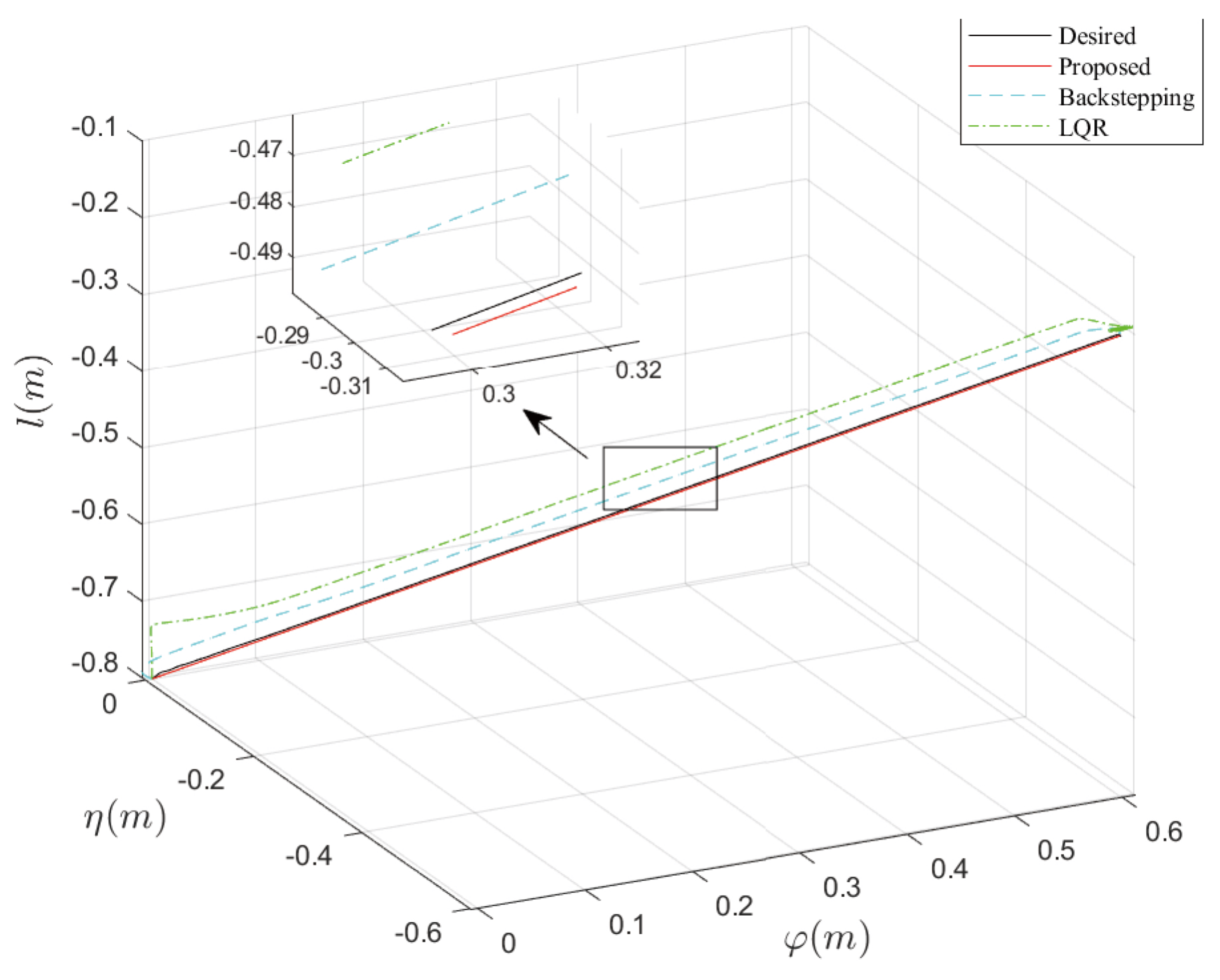
- As is known, this is a tracking controller designed for obstacle avoidance, enabling the payload to avoid obstacles of various shapes and reach the desired position.
- (2)
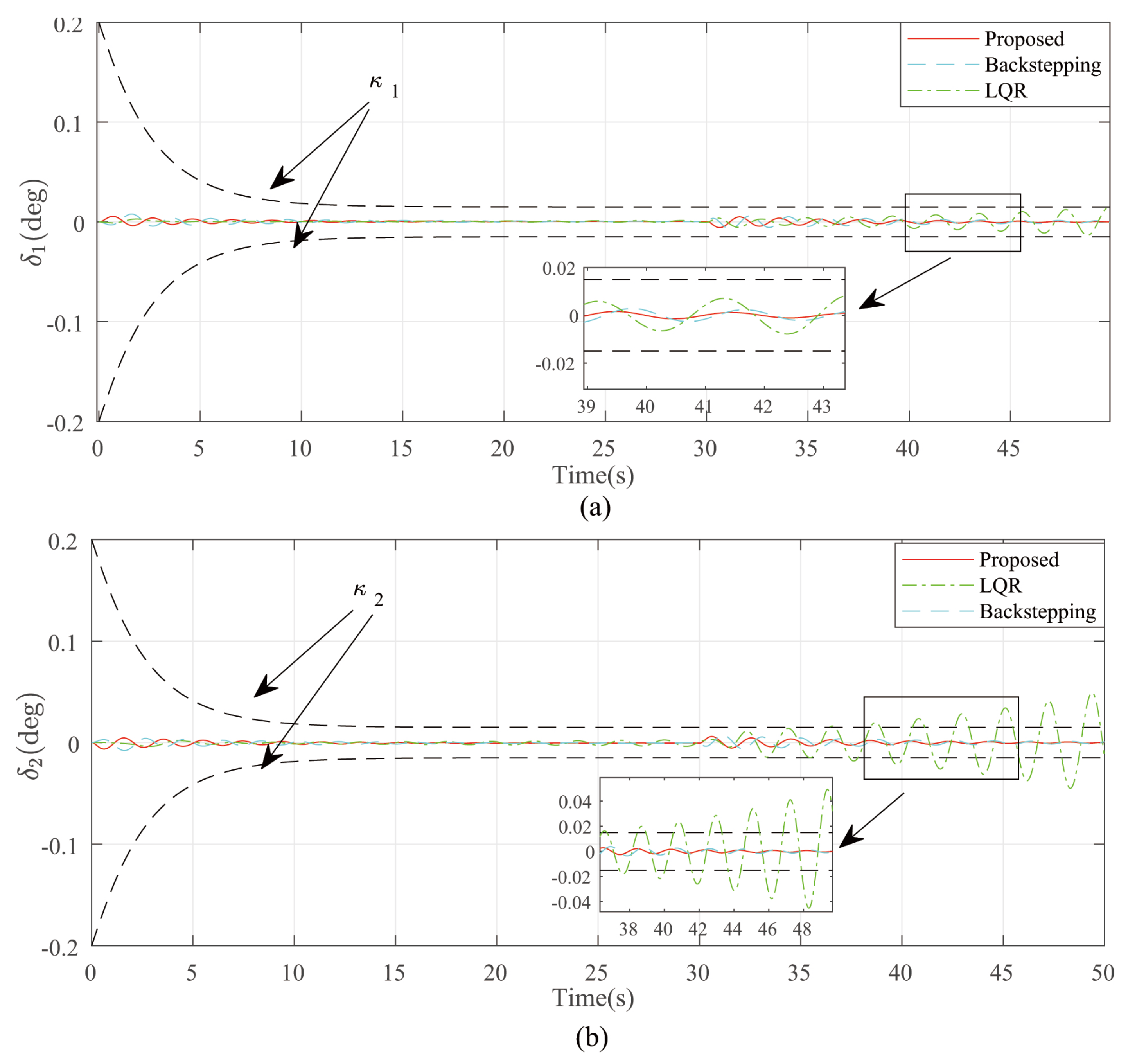
- The swing angles and are always constrained within the predefined boundaries and and they are asymptotically stable, which means
- (3)
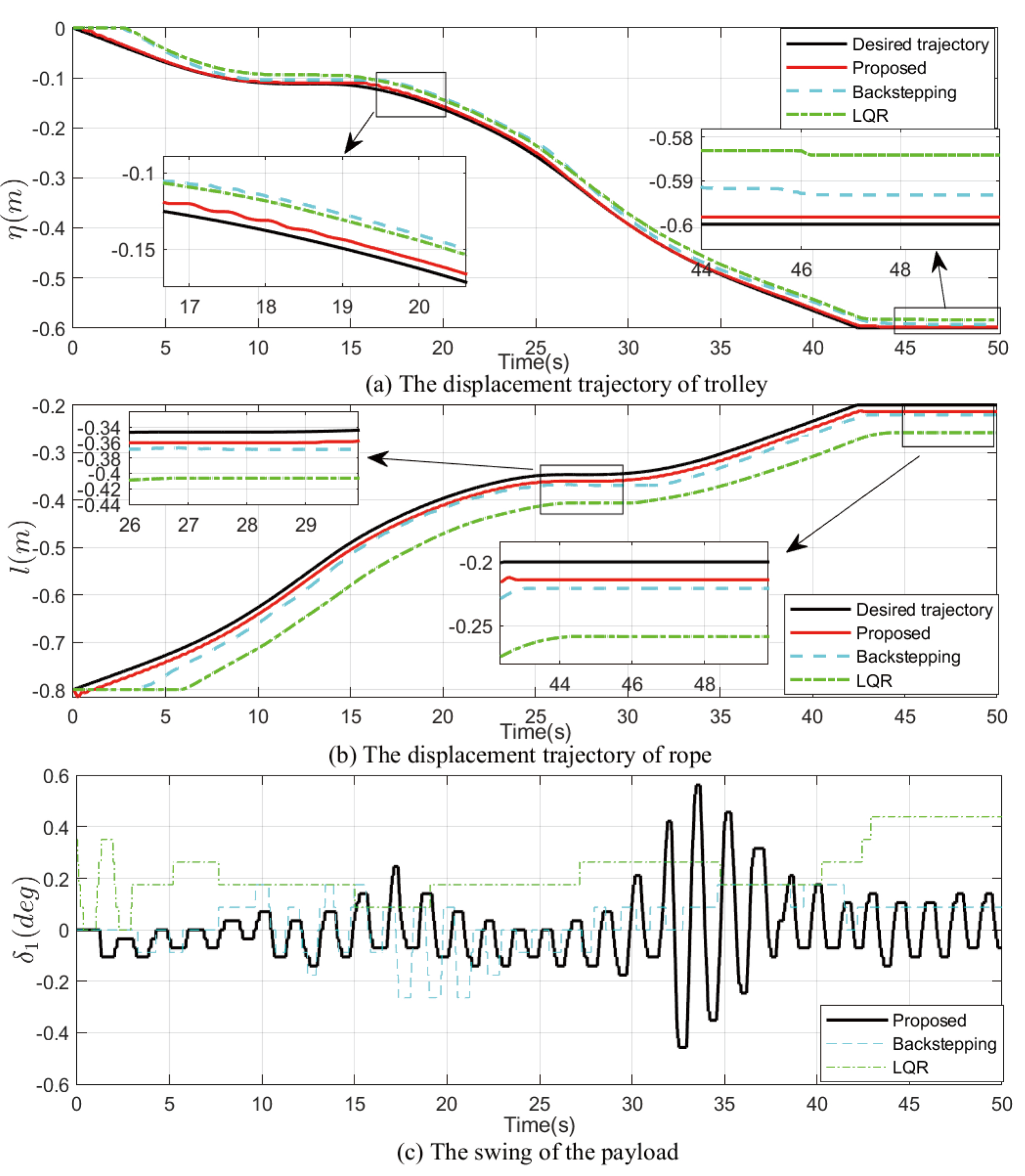
- The displacement of the trolley, movement of the bridge and length of the rope are asymptotically stable, which satisfy
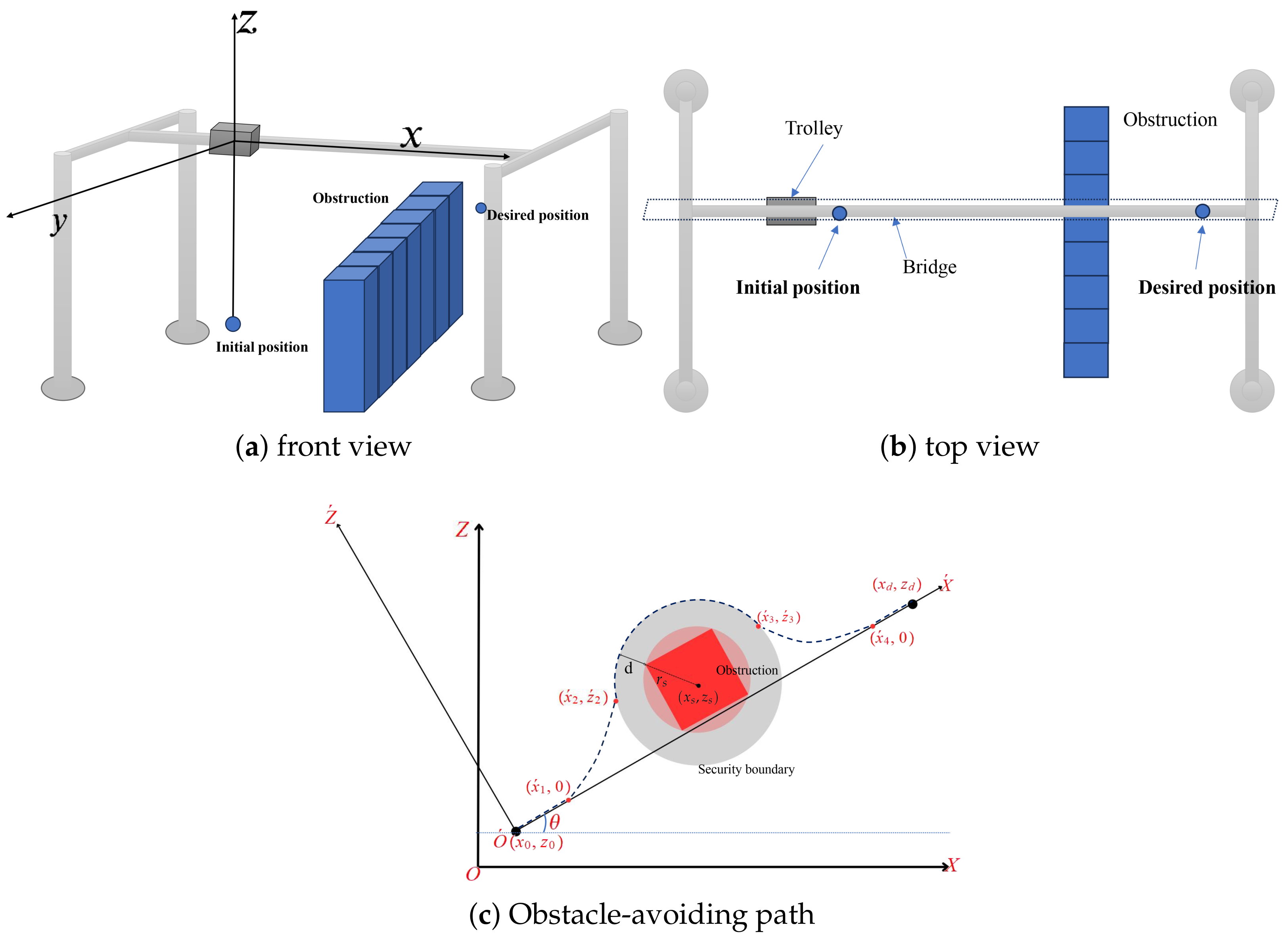
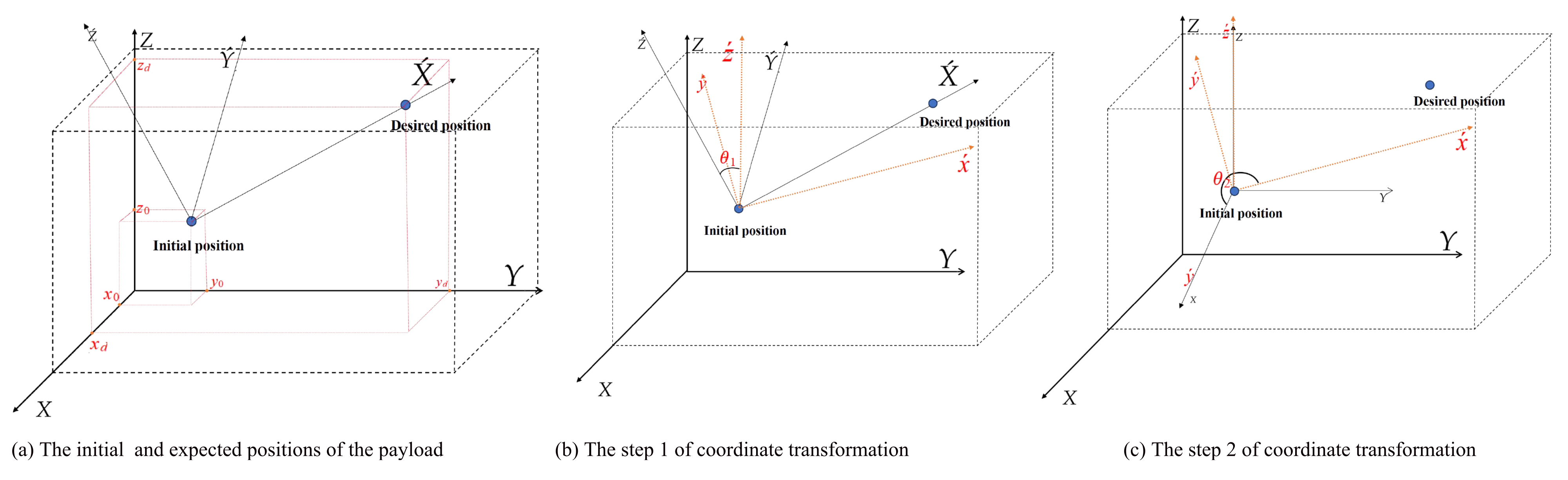
2.2. The Trajectory Modification
2.3. Swing Angle Constraint
3. Controller Design and Stability Analysis
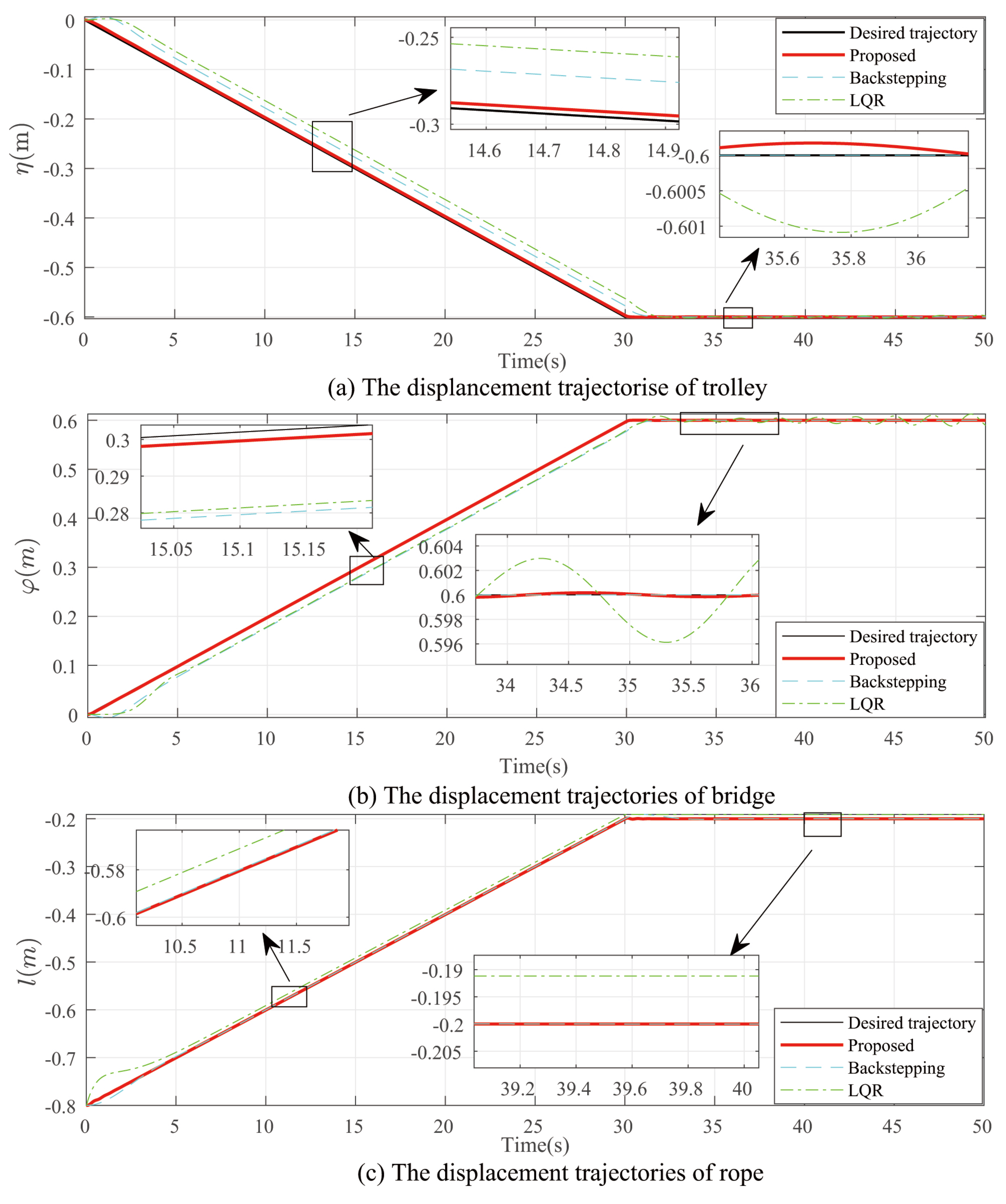
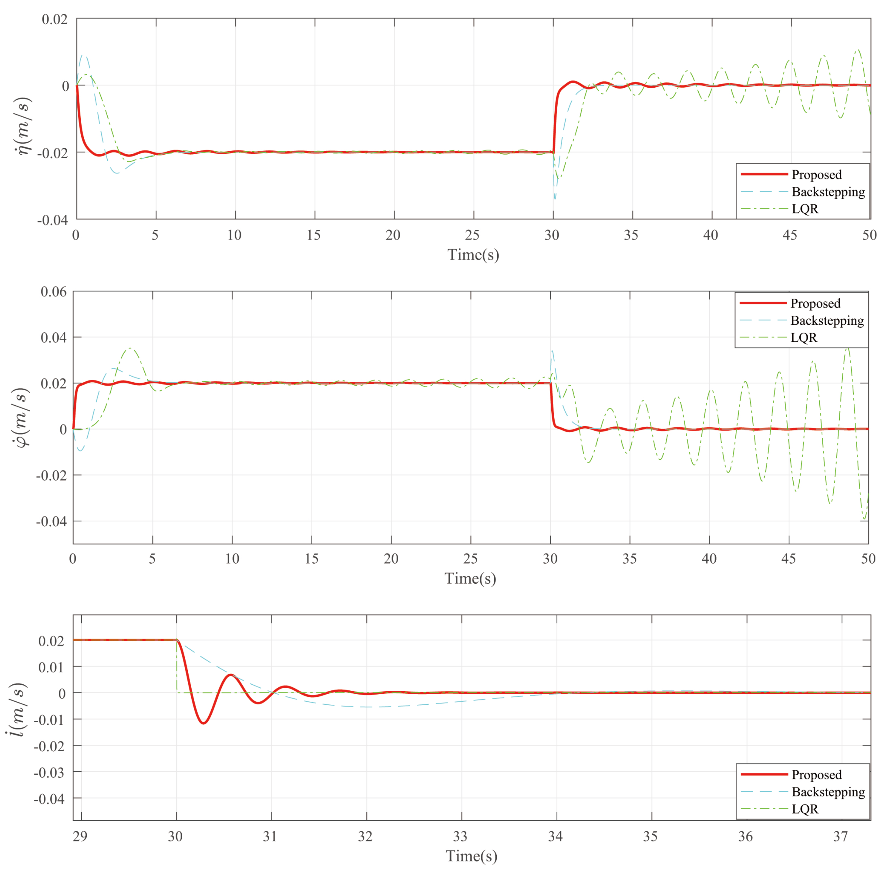
4. Experiment Result
4.1. Experiment 1
4.2. Experiment 2

5. Conclusions
Author Contributions
Funding
Data Availability Statement
Conflicts of Interest
Appendix A
References
- Chen, N.; Sun, H.; Fang, Y. Adaptive optimal motion control of uncertain underactuated mechatronic systems with actuator constraints. IEEE/ASME Trans. Mechatron. 2023, 28, 210–222. [Google Scholar] [CrossRef]
- Kim, G.-H.; Hong, K.-S. Adaptive sliding-mode control of an offshore container crane with unknown disturbances. IEEE/ASME Trans. Mechatron. 2019, 24, 2850–2861. [Google Scholar] [CrossRef]
- Liu, C.; Meng, S.; Liu, X.; Zhao, Y.; Wang, H.; Li, C. A tracking control method with the fast finite-time command filter for four degrees of freedom tower cranes. Trans. Inst. Meas. Control 2024, 47, 01423312241259066. [Google Scholar] [CrossRef]
- Chen, H.; Fang, Y.; Sun, N. A swing constraint guaranteed MPC algorithm for underactuated overhead Cranes. IEEE Trans. Ind. Electron. 2016, 21, 2543–2555. [Google Scholar] [CrossRef]
- Tang, W.; Ma, R.; Wang, W.; Gao, H. Optimization-based input-shaping swing control of overhead cranes Applied. Appl. Sci. 2023, 13, 9637. [Google Scholar] [CrossRef]
- Albalta, M.; Yalcin, Y. Model reference input shaped neuro-adaptive sliding mode control of gantry crane. Proc. Inst. Mech. Eng. Part J. Syst. Control. Eng. 2023, 237, 824–838. [Google Scholar] [CrossRef]
- Wu, Y.; Sun, N.; Chen, H.; Zhang, J.; Fang, Y. Nonlinear time-optimal trajectory planning for varying-rope-length overhead cranes. Assem. Autom. 2018, 38, 587–594. [Google Scholar] [CrossRef]
- Zhou, W.; Xia, X. Optimal motion planning for overhead cranes. IET Control Theory Appl. 2014, 8, 1833–1842. [Google Scholar]
- Fang, Y.; Ma, B.; Wang, P.; Zhang, X. A motion planning-based adaptive control method for an underactuated crane system. IEEE Trans. Control. Syst. Technol. 2012, 20, 241–248. [Google Scholar] [CrossRef]
- Yang, Y.; Zhang, T.; Zhou, X.; Zhang, H.; Li, J. Neural network adaptive PID-like coupling control for double pendulum cranes with time-varying input constraints. IEEE Trans. Neural. Netw. Learn. Syst. 2024, 208, 110997. [Google Scholar]
- Lai, J.; Huang, K.; Lu, B.; Zhao, Q.; Chu, H. Verticalized-tip trajectory tracking of a 3D-printable soft continuum robot: Enabling surgical blood suction automation. IEEE/ASME Trans. Mechatron. 2022, 27, 1545–1556. [Google Scholar]
- Zhang, S.; He, X.; Zhu, H.; Li, X.; Liu, X. PID-like coupling control of underactuated overhead cranes with input constraints. Mech. Syst. Signal Process. 2022, 178, 109274. [Google Scholar] [CrossRef]
- Fan, B.; Zhang, Y.; Sun, L.; Wang, L.; Liao, Z. Passivity and underactuated modeling-based load energy coupling control for three-dimensional overhead crane systems. Mechatronics 2023, 96, 103062. [Google Scholar]
- Yoshida, Y.; Tabata, H. Visual feedback control of an overhead crane and its combination with time-optimal control. In Proceedings of the 2008 IEEE/ASME International Conference on Advanced Intelligent Mechatronics, Xi’an, China, 2–5 July 2008; pp. 1114–1119. [Google Scholar] [CrossRef]
- Liu, R.; Li, S.; Chen, X. An optimal integral sliding mode control design based on pseudospectral method for overhead crane systems. In Proceedings of the 32nd Chinese Control Conference, Xi’an, China, 26–28 July 2013; pp. 2195–2200. [Google Scholar]
- Xu, W.; Xu, Y.; Zheng, X. Adaptive twisting sliding mode control for overhead cranes. In Proceedings of the 2015 IEEE International Conference on Cyber Technology in Automation, Control, and Intelligent Systems (CYBER), Shenyang, China, 8–12 June 2015; pp. 1379–1384. [Google Scholar] [CrossRef]
- Xu, W.; Zheng, X.; Liu, Y.; Zhang, M.; Luo, Y. Adaptive dynamic sliding mode control for overhead cranes. In Proceedings of the 2015 34th Chinese Control Conference (CCC), Hangzhou, China, 28–30 July 2015; pp. 3287–3292. [Google Scholar] [CrossRef]
- Zhang, Q.; Fan, B.; Wang, L.; Liao, Z. Fuzzy sliding mode control on positioning and anti-swing for overhead crane. Int. J. Precis. Eng. Manuf. 2023, 24, 1381–1390. [Google Scholar] [CrossRef]
- Shi, R.; Ouyang, H. Disturbance-observer-based discrete-time sliding mode predictive control for overhead cranes with matched and unmatched disturbances. Trans. Inst. Meas. Control 2024, 46, 1590–1600. [Google Scholar] [CrossRef]
- Huang, P.; Gu, H.; Hu, X.; Zhang, Z. Antiswing sliding mode control of overhead cranes with a finite-time disturbance observer. In Proceedings of the 2023 2nd Conference on Fully Actuated System Theory and Applications (CFASTA), Qingdao, China, 14–16 July 2023; pp. 149–154. [Google Scholar] [CrossRef]
- Wang, S.; Jin, W.; Zhang, X. Neural network–based adaptive sliding mode control of three-dimensional double-pendulum overhead cranes with prescribed performance. Trans. Inst. Meas. Control 2024. [Google Scholar] [CrossRef]
- Kim, T.D.; Nguyen, T.; Do, D.M.; Le, H.X. Adaptive neural network hierarchical sliding mode control for six degrees of freedom overhead crane. Asian J. Control 2023, 25, 2736–2751. [Google Scholar] [CrossRef]
- Sun, Z.; Sun, Z.; Xie, X. Parameter optimization of type II fuzzy sliding mode control for bridge crane systems based on improved grey wolf algorithm. Optim. Control. Appl. Methods 2024, 45, 2136–2152. [Google Scholar]
- Sun, N.; Fang, Y.; Zhang, X. Energy coupling output feedback control of 4-DOF underactuated cranes with saturated inputs. Automatica 2013, 49, 1318–1325. [Google Scholar] [CrossRef]
- Wu, X.; He, X. Nonlinear Energy-Based Regulation Control of Three-Dimensional Overhead Cranes. IEEE Trans. Autom. Sci. Eng. 2017, 14, 1297–1308. [Google Scholar] [CrossRef]
- Vazquez, C.; Fridman, L.; Collado, J. Second order sliding mode control of a 3-dimensional overhead-crane. In Proceedings of the 2012 IEEE 51st IEEE Conference on Decision and Control (CDC), Maui, HI, USA, 10–13 December 2012; pp. 6472–6476. [Google Scholar] [CrossRef]
- Deka, A.; Basireddy, S.R. Emergency braking control in 3D overhead cranes using a switching PD-fuzzy controller. In Proceedings of the 2023 9th International Conference on Control, Automation and Robotics (ICCAR), Beijing, China, 21–23 April 2023; pp. 285–290. [Google Scholar] [CrossRef]
- Hara, Y.; Noda, Y. Operational assistance system for obstacle collision avoidance and load sway suppression in overhead traveling crane. Proc. IEEE Int. Conf. Syst. Man. Cybern. 2016, 2196–2201. [Google Scholar] [CrossRef]
- Zhang, W.; Chen, H.; Chen, H.; Liu, W. A time optimal trajectory planning method for double-pendulum crane systems with obstacle avoidance. IEEE Access. 2021, 13022–13030. [Google Scholar] [CrossRef]
- Matsusawa, K.; Noda, Y.; Kaneshige, A. On-demand trajectory planning with load sway suppression and obstacles avoidance in automated overhead traveling crane system. In Proceedings of the 2019 IEEE 15th International Conference on Automation Science and Engineering (CASE), Vancouver, BC, Canada, 22–26 August 2019; pp. 1321–1326. [Google Scholar] [CrossRef]
- Inomata1, A.; Noda, Y. Fast trajectory planning by design of initial trajectory in overhead traveling crane with considering obstacle avoidance and load vibration suppression. In Proceedings of the 13th International Conference on Motion and Vibration Control (MOVIC 2016) and the 12th International Conference on Recent Advances in Structural Dynamics (RASD 2016), Southampton, UK, 4–6 July 2016. [Google Scholar] [CrossRef]
- Iftikhar, S.; Faqir, O.J.; Kemgan, E.C. Nonlinear model predictive control of an overhead laboratory-scale gantry crane with obstacle avoidance. In Proceedings of the 2019 IEEE Conference on Control Technology and Applications (CCTA), Hong Kong, China, 19–21 August 2019; pp. 382–387. [Google Scholar] [CrossRef]
- Gutierrez, I.; Collado, J. An LQR controller in the obstacle avoidance of a two-wires hammerhead crane. Neurocomputing 2017, 233, 14–22. [Google Scholar] [CrossRef]
- Zhu, H.; Ouyang, H.; Xi, H. Neural network-based time optimal trajectory planning method for rotary cranes with obstacle avoidance. Mech. Syst. Signal Process. 2023, 185, 109777. [Google Scholar] [CrossRef]
- Zhao, Y.; Li, W.; Wang, X.; Yi, C. Predefined-time bounded consensus of multiagent systems with unknown nonlinearity via distributed adaptive fuzzy control. Math. Probl. Eng. 2019, 185, 7621464. [Google Scholar] [CrossRef]
- Bettega, J.; Richiedei, D.; Tamellin, I. Trajectory planning through model inversion of an underactuated spatial gantry crane moving in structured cluttered environments. Actuators 2024, 13, 176. [Google Scholar] [CrossRef]
- Ma, B.; Fang, Y.; Zhang, X.; Wang, X. Modeling and simulation for a 3D overhead crane. In Proceedings of the 2008 7th World Congress on Intelligent Control and Automation, Chongqing, China, 25–27 June 2008. [Google Scholar]
- Ren, H.R.; Lu, R.Q.; Xiong, J.L.; Wu, Y.Q.; Shi, P. Nonlinear Systems, 3rd ed.; Prentice Hall: Upper Saddle River, NJ, USA, 2002. [Google Scholar]


| Parameter | Physical Meaning | Unit |
|---|---|---|
| trolley translation displacement | m | |
| displacement of bridge | m | |
| l | cable length | m |
| payload swing angle in the x direction | rad | |
| payload swing angle in the y direction | rad | |
| trolley mass | kg | |
| mass of trolley and bridge | kg | |
| m | payload mass | kg |
| g | gravity acceleration constant | m/s2 |
| translation control force of trolley | N | |
| translation control force of bridge | N | |
| hoisting/lowering actuating force | N | |
| , | coefficients of sliding friction | N |
| , , , | position of the load center of payload | m |
| , , | resistance coefficients | / |
| coefficients of air resistance | / |
Disclaimer/Publisher’s Note: The statements, opinions and data contained in all publications are solely those of the individual author(s) and contributor(s) and not of MDPI and/or the editor(s). MDPI and/or the editor(s) disclaim responsibility for any injury to people or property resulting from any ideas, methods, instructions or products referred to in the content. |
© 2025 by the authors. Licensee MDPI, Basel, Switzerland. This article is an open access article distributed under the terms and conditions of the Creative Commons Attribution (CC BY) license (https://creativecommons.org/licenses/by/4.0/).
Share and Cite
Meng, S.; He, W.; Liu, N.; Zhang, R.; Liu, C. Couple Anti-Swing Obstacle Avoidance Control Strategy for Underactuated Overhead Cranes. Actuators 2025, 14, 90. https://doi.org/10.3390/act14020090
Meng S, He W, Liu N, Zhang R, Liu C. Couple Anti-Swing Obstacle Avoidance Control Strategy for Underactuated Overhead Cranes. Actuators. 2025; 14(2):90. https://doi.org/10.3390/act14020090
Chicago/Turabian StyleMeng, Shuo, Weikai He, Na Liu, Rui Zhang, and Cungen Liu. 2025. "Couple Anti-Swing Obstacle Avoidance Control Strategy for Underactuated Overhead Cranes" Actuators 14, no. 2: 90. https://doi.org/10.3390/act14020090
APA StyleMeng, S., He, W., Liu, N., Zhang, R., & Liu, C. (2025). Couple Anti-Swing Obstacle Avoidance Control Strategy for Underactuated Overhead Cranes. Actuators, 14(2), 90. https://doi.org/10.3390/act14020090