Article

Nonlinearity Harmonic Error Compensation Method Based on Intelligent Identification for Rate Integrating Resonator Gyroscope

1
School of Instrumentation and Optoelectronic Engineering, Beihang University, Beijing 100191, China
2
School of Mechanical Engineering, Zhejiang University, Hangzhou 310058, China
3
College of Marine Equipment and Mechanical Engineering, Jimei University, Xiamen 361021, China
*
Author to whom correspondence should be addressed.
Actuators 2025, 14(2), 68; https://doi.org/10.3390/act14020068
Submission received: 19 December 2024 / Revised: 25 January 2025 / Accepted: 26 January 2025 / Published: 3 February 2025
(This article belongs to the Section Precision Actuators)

Abstract

:
This paper presents an improved intelligent optimizing algorithm based on parameter identification and drift compensation for the rate-integrating resonator gyroscope (RIRG). Besides damping and frequency imperfections, the RIRG measurement accuracy still suffers from limitations due to nonlinear error. Therefore, the dynamic nonlinear error model for RIRG has been established to reveal the relationship between the pattern angle and harmonic drifts. Based on this, a dynamic analysis of the gyroscope operating state is carried out using nonlinear motion equations. The optimal harmonic error parameters are then identified by a particle swarm optimization (PSO) algorithm for the drift error compensation. To further improve the measurement accuracy, chaotic technology is integrated with PSO, leading to more precise identification. Subsequently, the harmonic parameters of the bias drifts are efficiently compensated. Experimental results demonstrate that the bias drift is reduced by over 90% after harmonic error compensation, demonstrating the validity of the proposed method in enhancing the measurement accuracy of RIRGs.

1. Introduction

Rate integrating resonator gyroscopes (RIRGs) represent a kind of resonant gyroscope that has been adequately discussed and extensively applied within the inertial navigation community. These gyroscopes exhibit characteristics such as direct angular measurement and unlimited dynamic range [1,2]. The accuracy of the RIRG does not depend on the dimensions of the resonator, but rather on the material mechanism and manufacturing process, which can lead to two major types of errors in vibration: damping asymmetry and frequency mismatch [3]. The requirements for suppressing instability in high-precision applications are necessary, encompassing more demands on the complexity of the control system and the accuracy of the error analysis.
The relationship between the control strategy and the characteristic variables of the resonator could be described by the dynamic model equations related to damping asymmetry and frequency mismatch. Due to these errors, the output of the angle measurement contains multiple harmonic error terms correlated with the standing wave pattern angle [4,5].
For the purpose of reducing angular drifts, sophisticated control algorithms and imperfections compensation approaches have attracted lots of research interest. V. Apostolyuk [6] presented a synthesis of a feedback controller aimed at reducing measurement drifts. Ryunosuke Gando [7] and Kechen Guo [8] utilized a feed-forward damper to adjust the resistance and voltage for compensating damping asymmetry. Siamak Zargari [9] proposed an additional feedback path to decrease the quadrature error in the readout circuit. Parsa Taheri-Tehrani [10] and Jiangkun Sun [11] paid more attention to the relationship between the actuation gain and angular errors resulting from the electrode misalignment and the gap asymmetry. Ruan [12] manipulated a proportional-integral resonance controller instead of traditional proportional-integral controllers to automatically eliminate frequency mismatch.
All of the above studies were conducted based on a linear dynamic model. However, it has been shown in the literature [13,14,15] that there may exist fourth harmonic components present in the drift error. To comprehensively explore the dynamics of the RIRG system when operating beyond the linear region, it is essential to adopt a model including the nonlinear damping and stiffness contributions.
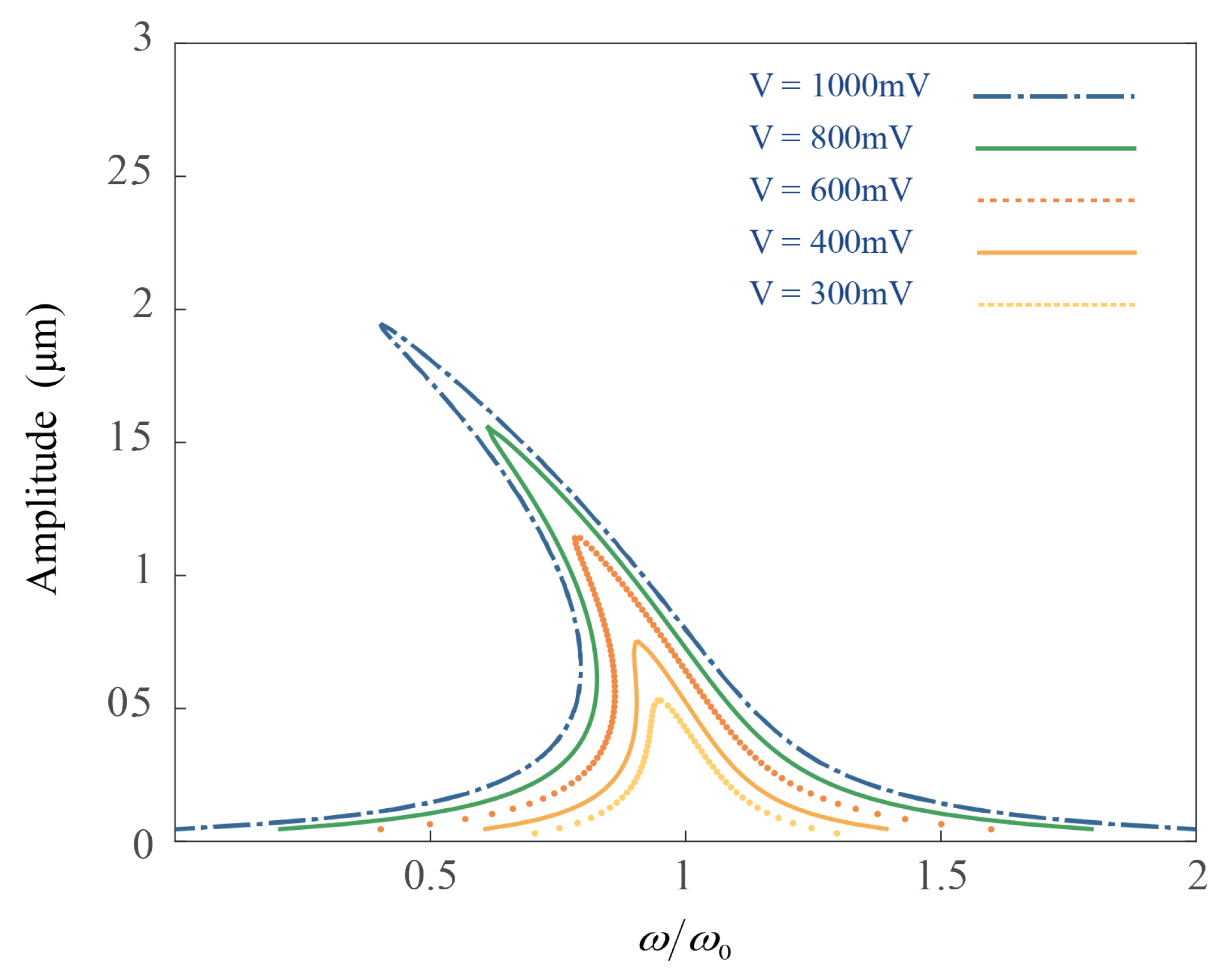
The nonlinear errors in RIRGs arise from multiple sources. Firstly, the use of flat electrodes for detection and actuation induces electrostatic spring-softening nonlinearity, leading to cubic nonlinearities. Additionally, the mechanical nonlinearity of the structure itself results in the Duffing nonlinearity. Extensive studies have documented the nonlinear response and bifurcation phenomena of resonators due to elastic and damping nonlinearities [16,17,18]. Among the most commonly reported nonlinear effects is the amplitude–frequency response induced by Duffing nonlinearity. Several innovative techniques have been proposed to mitigate these effects, including the application of tuning voltages to adjust frequency mismatches dependent on bifurcation thresholds [16], the use of capacitance corrections based on linearization factors [18,19], and the identification of amplitude-dependent correction gains to counteract nonlinearities in capacitive detection [20]. Furthermore, nonlinearity originating from electrostatic transduction and capacitance gap nonuniformity complicates the relationship between the RIRG input and output [21]. Given the correlation between harmonic errors and the standing wave pattern angle, an effective approach for precise angular measurement involves establishing a high-accuracy dynamic output compensation model for the RIRG. Therefore, the accuracy of parameter identification is crucial for the implementation of the nonlinearity harmonic error compensation.
Artificial intelligence has been gradually applied to various fields, including resonator gyroscopes. Xia et al. integrated a Fuzzy-PID controller with a BP neural network for the temperature control system of micro-gyroscopes, ensuring temperature stability [22]. H. Yu et al. developed a capacitance-pose inverse model using a BP neural network to enhance the capacitance uniformity of RIRGs [23]. Y. Li et al. proposed a genetic algorithm to optimize the dynamic output decomposition of resonator gyroscopes [24].
Particle swarm optimization (PSO) is one of the intelligent swarm optimization algorithms which has good nonlinear optimization ability and variable recognizing ability [25]. An improved PSO algorithm introduces chaos mapping which is used to enhance the distribution diversity of population particles, enabling more efficient and accurate parameter identification.
In this paper, considering the nonlinearities of the resonator, we develop a resonator motion model to analyze the effects of these errors on the threshold range of RIRG angular velocity and establish the relationship between the vibration pattern angle and the dynamic output drift errors of the RIRG. To denoise the RIRG output, we propose an improved particle swarm optimization (IPSO) algorithm based on chaos mapping for harmonic parameter identification aimed at compensating for the RIRG output drift. The effectiveness of the proposed IPSO-based parameter identification and drift compensation is validated through the simulation of the entire nonlinear RIRG control system. The performance of the compensation is evaluated by comparing the original drift error of the RIRG with the drift error corrected using the harmonic parameters identified by IPSO.
The following sections of this paper are organized as follows: Section 2 presents an analysis of the dynamic model of the RIRG system containing nonlinear coefficient terms. 
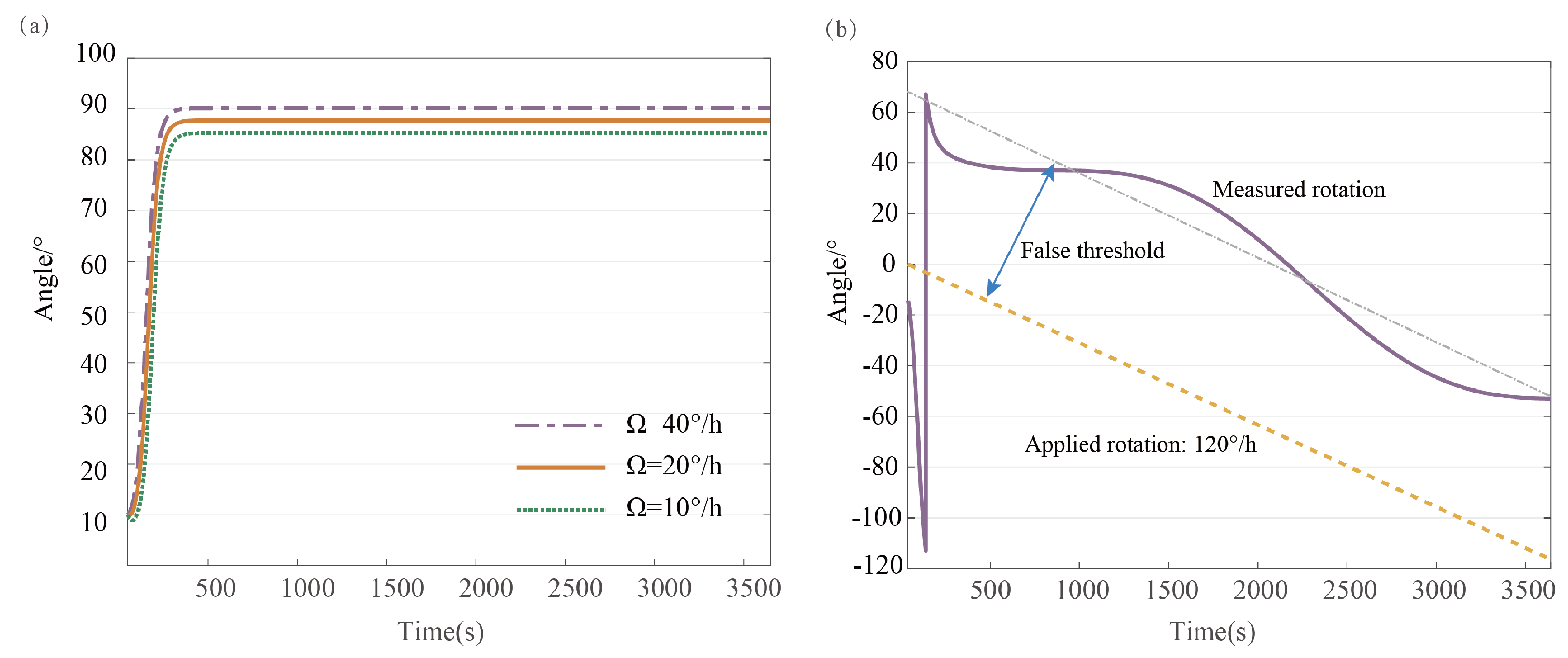
Section 3 discusses the threshold obstacle and the angle output distortion problem of RIRG in the nonlinear region based on the angular error equation. Section 4 details the use of the IPSO algorithm to estimate the parameters. The results of the simulation and experimental studies on closed-loop control are presented in Section 5. Section 6 provides a summary of the findings of the study.

2. Establishment of Nonlinear Dynamic Model

2.1. Nonlinearity Oscillator Model

Duffing’s oscillator, which describes the nonlinear vibration behavior of many electrical and mechanical systems, could be expressed by Duffing’s equation,
x ¨ + 2 τ + γ x 2 x ˙ + ω 0 x 2 + α x 3 = F cos ω t
where x represents the vibration displacement of the oscillator, τ represents the damping factor, γ = β A C 0 V d c β A C 0 V d c m d m d is the nonlinear dissipation term for the damping of the system leading to non-exponential decay, α = 2 C 0 V d c 2 2 C 0 V d c 2 m d m d represents the nonlinear spring constant ( C 0 is the nominal capacitance of the flat electrode, V d c is the DC voltage, d is the electrode gap, n is the equivalent mass of the resonator, β is the detection gain, and A is the detection gain), both of which would cause a bifurcation of the amplitude-dependent effect, and it is usually impossible to accurately extract these parameters from a single frequency sweep. The frequency of excitation ω is tuned close to the fundamental mode of mechanical vibrations.
The distinction between nonlinear and linear vibrations lies in the variability of frequency and amplitude. In weakly nonlinear systems, this variability is subtle, manifesting primarily when the system time significantly exceeds the vibration period. Consequently, the amplitude changes in nonlinear systems exhibit a “slow-varying” nature and the dynamics of the resonator ringdown response can be studied in terms of Lynch’s “averaging” method.
Moreover, the prerequisite for the feasibility of equivalent linearization in weakly nonlinear vibrations is the approximate adherence to simple harmonicity. There is not an analytical solution in the nonlinear Equation (1); the ingress method is employed to obtain the approximate analytical solution, particularly under the condition of weak nonlinearity within the system. The amplitude and phase of the oscillator vibration can be expressed as the following equations:
a ˙ = 1 τ + 1 2 γ a 2 a + 1 2 F sin ϕ ϕ ˙ = Δ ω + 3 α 8 ω 0 a 2 + 1 2 a F cos ϕ
where a is the vibration amplitude, ϕ is the vibration phase, Δ ω is the detuning parameter, F is the constant electrostatic force.
The frequency–amplitude pairs are measured at five values of electrostatic force, ranging from 300 to 1000 mV, and then frequency-to-amplitude response curves are constructed. As seen in Figure 1, the amplitude–frequency characteristic of the resonator vibration significantly changes with variations in amplitude and frequency mismatch. With increasing excitation force, the vibration amplitude gradually rises.
According to Figure 1, the nonlinear amplitude–frequency response analysis of the forced vibration Duffing equation reveals the following features:
(1)
The presence of the nonlinear spring constant leads to a leftward bend in the amplitude–frequency characteristic curve of the resonator. As the excitation amplitude increases, the amplitude–frequency curve in nonlinearity space induces the emergence of a multivalued region, resulting in jump instability and hysteresis behavior in open-loop oscillations. For closed-loop resonators, stable operation above the critical amplitude is guaranteed despite the presence of nonlinearities.
(2)
Nonlinear damping may originate from both mechanical and electrical factors. The electrostatic nonlinearity induced by parallel-plate electrodes is associated with soft-spring damping nonlinearity, and the nonlinear damping arising from geometrical and material aspects is associated with hard-spring damping nonlinearity. However, as a kind of high-quality factor resonator, the effect of geometrical and material nonlinearities on RIRG angular drift is negligible compared to the nonlinearity stemming from the electrostatic transduction.

2.2. Nonlinear Dynamic Model of Resonant Gyroscope

RIRG is a kind of two-degree-of-freedom resonant gyroscope. The second-order modal vibration of RIRG can be equated to the simple harmonic vibration of a mass block in two-dimensional space. In the linear case, the dynamic equation contains the frequency mismatch and the damping anisotropy errors. Based on the mathematical modeling of non-ideal RIRG derived by Lynch, the damping dissipation error and the Duffing error discussed above are taken into consideration, and the governing motion equation can be written as
x ¨ y ¨ + 2 K Ω U + 2 τ I + Δ 1 τ cos 2 θ τ V + Δ 1 τ sin 2 θ τ W x ˙ y ˙ + ω 2 ω Δ ω cos 2 θ ω V ω Δ ω sin 2 θ ω W x y + γ x 2 0 0 y 2 x ˙ y ˙ + α 1 1 / 2 1 / 2 1 x 2 0 0 y 2 x y = f x f y
where x and y represent the generalized displacement of oscillator in the two-dimensional space. I = 1 0 0 1 , U = 0 1 1 0 , V = 1 0 0 1 , W = 0 1 1 0 . τ x and τ y are damping coefficients, 2 2 τ τ = 1 1 τ x + τ x + 1 1 τ y τ y stands for the average time constant, Δ 1 1 τ τ = 1 1 τ x τ x 1 1 τ y τ y stands for the damping anisotropy. If τ x < τ y , θ τ denotes the angle of the damping axis and the X-axis. ω stands for the natural resonator frequency, ω x and ω y are the resonant frequency of two vibration modes, Δ ω = ω x 2 ω y 2 ω x 2 ω y 2 2 ω 2 ω stands for the frequency mismatch. If ω x < ω y , θ ω denotes the angle of the frequency axis and the X-axis. f x and f y are the forces applied for the control electrodes of the resonator. Ω is true input rate with gain factor K. γ and α are electrostatic damping nonlinearity and nonlinear spring constant.
The standing wave of the two-degree-freedom resonant gyroscope is in the form of a four-wave belly and generates a reverse procession under the external excitation. The shape of the standing wave can be decomposed into two ellipses along two orthogonal axes, where the four endpoints of the long axes of the two ellipses are called the antinode points and the intersection of the two ellipses is called the node point. The concept of RIRG is shown in Figure 2.
To obtain the variational vibration of the resonator, elliptic parameters are used to represent the signals of two orthogonal electrodes.
x = a cos θ cos ω t + φ q sin θ sin ω t + φ x ˙ = ω a cos θ sin ω t + φ + q sin θ cos ω t + φ y = a sin θ cos ω t + φ + q cos θ sin ω t + φ y ˙ = ω a sin θ sin ω t + φ q cos θ cos ω t + φ
where a, q are amplitudes of the major and minor vibration modes, θ is the vibration pattern angle, ω is the natural resonator frequency, ϕ is the initial phase of the vibration mode.
The effect of each error term on the output of the resonant gyroscope is analyzed by converting the equations into the form of elliptic parametric equations using the dynamic modal. A vector–matrix differential equation satisfying the following form is put forward to obtain solutions of elliptic orbit parameters:
z ˙ = A z + f z
where z t = g t , h t and the trend of vector h t represents the changing displacement of resonator vibration.
Therefore, a series of one-dimensional differential equations can be obtained by solving this differential equation above.
a ˙ = q 2 Δ ω sin 2 θ θ ω a 1 τ + 1 2 Δ 1 τ cos 2 θ θ τ 3 γ 16 a 3 γ 16 a q 2 γ 16 a a 2 q 2 cos 4 θ α 2 ω 3 a 2 q 16 + q 3 16 + q a 2 q 2 8 s i n 4 θ + 1 2 cos 4 θ ,
q ˙ = a 2 Δ ω sin 2 θ θ ω q 1 τ 1 2 Δ 1 τ cos 2 θ θ τ 3 γ 16 q 3 γ 16 a 2 q + γ 16 q a 2 q 2 cos 4 θ + α 2 ω 3 a 3 16 + a q 2 16 + a a 2 q 2 8 s i n 4 θ + 1 2 cos 4 θ ,
θ ˙ = a q Δ ω a 2 q 2 cos 2 θ θ ω + a 2 + q 2 Δ 1 1 τ τ 2 a 2 q 2 sin 2 θ θ τ K Ω + α a q 2 ω 1 4 + 1 4 cos 4 θ 1 8 sin 4 θ 3 γ 32 a 2 + q 2 sin 4 θ ,
φ ˙ = a 2 + q 2 Δ ω 2 a 2 q 2 cos 2 θ θ ω a q Δ 1 1 τ τ 2 a 2 q 2 sin 2 θ θ τ α a 2 + q 2 2 ω 9 16 + 3 16 cos 4 θ 3 16 sin 4 θ + 3 γ a q 8 sin 4 θ + ω
where γ = γ 31 .
Dynamic Equations (6)–(9) describe the influence of nonlinearities on all four state variables of the angular procession of RIRG in the elliptic frame.
The sensed angular change is related to four parts: the input rate, damping asymmetry, frequency mismatch, and damping nonlinearity. Since the frequency mismatch is suppressed by the quadrature loop, the main error in the angular measurement is caused by the damping asymmetry and damping nonlinearity.
θ ˙ = K Ω + 1 2 Δ 1 τ sin 2 θ θ τ 3 32 γ a 2 sin 4 θ
According to Equation (10), a superposition of periodically varying functions occurs in the measurement result. The asymmetry damping coefficient results in a 2- θ dependent drift error and the nonlinear damping causes the gyroscope output to contain the fourth harmonic of the pattern angle.

3. Nonlinear Effects on Angular Drift Errors

Based on the angular error equation, the RIRG output analytical solution is discussed separately for diverse magnitudes of input angular velocity.

3.1. Threshold Effect with Nonlinearity Affection

Since there are two types of damping error terms in the angular output, the threshold effect needs to be discussed in two cases.
When Ω min Δ 1 1 τ τ Δ 1 1 τ τ K K , 3 a 2 γ 3 a 2 γ 16 K 16 K , the RIRG angular output can be written as
θ = a r c t Δ 1 1 τ τ K Ω u 1 + 2 u 1 2 u 1 1 C 1 exp 2 K Ω u 1 t 1 C 1 exp 2 K Ω u 1 t + a r c t a 2 γ 2 K Ω v 1 + 2 v 1 2 v 1 1 C 2 exp 2 K Ω v 1 t 1 C 2 exp 2 K Ω v 1 t + θ τ
where u 1 = Δ 1 1 τ τ Δ 1 1 τ τ K Ω K Ω 2 1 , v 1 = 3 a 2 γ 3 a 2 γ 16 K Ω 16 K Ω 2 1 , C 1 = 1 2 u 1 2 u 1 tan θ τ Δ 1 1 τ τ Δ 1 1 τ τ K Ω K Ω + u 1 tan θ τ Δ 1 1 τ τ Δ 1 1 τ τ K Ω K Ω + u 1 , C 2 = 1 2 v 1 2 v 1 a 2 γ a 2 γ 8 K Ω 8 K Ω + v 1 a 2 γ a 2 γ 8 K Ω 8 K Ω + v 1 .
Considering the effect of damping anisotropy is more significant than damping nonlinearity, the threshold value is dominated by the damping anisotropy error. This result shows analytically that the threshold range for rotation rates extends under the nonlinear condition compared with the linear condition and the RIRG effectively fails to operate. The performance of the resonator gyroscope is shown in Figure 3a.
On the other hand, when 3 a 2 γ 3 a 2 γ 16 K 16 K Ω Δ 1 1 τ τ Δ 1 1 τ τ K K , the RIRG angular output can be written as
θ = a r c t Δ 1 1 τ τ K Ω u 1 + 2 u 1 2 u 1 1 C 1 exp 2 K Ω u 1 t 1 C 1 exp 2 K Ω u 1 t + θ τ 1 2 K Ω v 2 t C 4 3 a 2 γ 32 K Ω 1 + cos 2 K Ω t + C 4
where v 2 = 1 3 a 2 γ 3 a 2 γ 16 K Ω 16 K Ω 2 , C 4 = 3 a 2 γ 3 a 2 γ 32 K Ω 32 K Ω 1 + cos 2 θ 0 cos 2 θ 0 2 2 .
As shown in Figure 3b, the angular output value is unable to fully respond to the input signal, but there is a hysteresis caused by a linear function with a periodic function with amplitude 3 a 2 γ 3 a 2 γ 32 K Ω 32 K Ω and slope K Ω 1 3 a 2 γ 3 a 2 γ 16 K Ω 16 K Ω 2 . At this moment, the measurement property of the resonator gyroscope is in the partial threshold−restricted region.
For the RIRG threshold obstacle, an excitation force is applied to the angular velocity control loop to realize the virtual rotation of the standing wave, which can act as a constant rate to overcome the threshold of the gyroscope [5,11,14].

3.2. Drift Error with Nonlinearity Affection

When Ω max Δ 1 1 τ τ Δ 1 1 τ τ K K , 3 a 2 γ 3 a 2 γ 16 K 16 K ,
θ = θ τ + Δ 1 1 τ τ 2 K Ω 1 + cos K Ω u 2 t + 2 C 3 1 2 K Ω u 2 t 3 a 2 γ 32 K Ω 1 + cos 2 K Ω v 2 t + C 4 1 2 K Ω v 2 t C 3 C 4
where u 2 = 1 Δ 1 1 τ τ Δ 1 1 τ τ K Ω K Ω 2 , C 3 = θ τ θ 0 + Δ 1 1 τ τ Δ 1 1 τ τ 2 K Ω 2 K Ω 1 + 2 cos 2 θ 0 .
Equation (13) indicates that the angular output of the resonant gyroscope contains a linear accumulation drift and a period drift, both of which are determined by the combined effects of the damping anisotropy and the damping nonlinearity components.
Figure 4 shows that the components of angular velocity drift incorporate higher-order harmonic errors. The second harmonic error is generated by the linear system including damping anisotropy, and the angular velocity measurement error exhibits a fourth harmonic distribution due to damping nonlinearity. As illustrated in the figure, the periodic drifts of the RIRG are correlated with the location of the standing wave and dependent on the magnitude of the damping anisotropy parameter and damping nonlinearity parameter.
From the previous discussion, it can be learned that the measurement accuracy of gyroscopes is limited by the linear damping dissipation term versus the nonlinear damping dissipation term when the frequency mismatch error is well suppressed under quadrature control. According to Equation (6), the trend of major vibration amplitude is also affected by the damping nonlinearity. In the nonlinear domain, the nonlinearity of the amplitude is more pronounced as the applied force increases. Considering damping nonlinearity is introduced by state feedback, an energy compensation control loop is used to overcome the effect of damping and maintain the amplitude of the resonator to a constant level.
The coupling of the damping nonlinearities makes it difficult to analyze the drift error mechanism accurately and establish a realistic compensation model. To solve these difficulties, we propose the parameter identification method to compensate for the RIRG dynamic output error comprehensively.

4. Harmonic Error Parameter Intelligent Identification and Compensation Method

In order to eliminate the error induced by the damping relevant error terms, a signal varying with the pattern angle is generated as compensation. The key to the compensation method is to estimate the RIRG’s damping asymmetry and damping nonlinearity parameters and exert the angle-dependent signal into the angular output loop. Equation (10) explains that linear error induces second harmonic drifts, whereas nonlinear error leads to fourth harmonic changes. Therefore, the output form of the resonant standing wave motion is a superposition of multiple harmonics. Since whichever drifts discussed in this chapter are angle-dependent, for inertial measurement devices such as RIRG, which have a periodic pattern of their errors, the locomotor position of the standing wave can be utilized to achieve the identification of the error parameter of the RIRG. The physical significance of the error parameters to be identified indicates the dominance of the output angular error. The angle-dependent signal to be recognized can be written as
u θ = a 1 sin 2 θ + b 1 cos 2 θ + a 2 sin 4 θ + b 2 cos 4 θ
where vector u = a 1 b 1 a 2 b 2 T represents the harmonic error components.
For minimizing multiple harmonics variations caused by angle drift, it is significant to set the right amount of compensation signal. After the measurements of the RIRG are made as described previously, these angle output data are used to evaluate the parameters in the nonlinearity harmonic model.

4.1. LSM-Based Identification of Parameters for the Nonlinear Harmonic Model

The most widely used estimation method in the field of parameter identification is the least squares method (LSM). The advantage of LSM is the simplicity of the algorithm, and theoretically, the accuracy of its parameter estimates increases with the increase of observed data.
To reflect the time-varying characteristics of the parameters during the identification period, a forgetting factor is further introduced, which is to ensure that the influence of the previous data on parameter identification is smaller than that of the current data, so that the time-varying parameters can be better tracked. In addition, a damping factor is introduced to avoid the bursting phenomenon of the recognized parameters.
g ^ m = g ^ m 1 + λ μ P m g ^ m 1 g ^ m 2 + P m h m T y m h m g ^ m 1
P m = μ I + λ H m 1 T W m 1 H m 1 + h m T h m 1
where λ and μ are the damping coefficient and forgetting factor.
However, the optimal metric for the LSM is the minimization of the sum of the estimated mean square errors of the measurement-based and does not ensure that the parameter identification errors are optimal, so the identification accuracy is not enough. In this paper, we propose an IPSO method to identify the harmonic parameters based on chaos mapping. This method eliminates the linear and nonlinear distribution of the angular velocity drift signals without affecting the feedback control parameters. IPSO can identify the unknown parameters so that we can set a virtual angle output loop with the estimate of the parameter vector and generate the compensation signal based on the identification. The IPSO method does not replace the PID control loops for the control of the major axis, minor axis, and resonance tracking.

4.2. IPSO-Based Identification of Parameters for the Nonlinear Harmonic Model

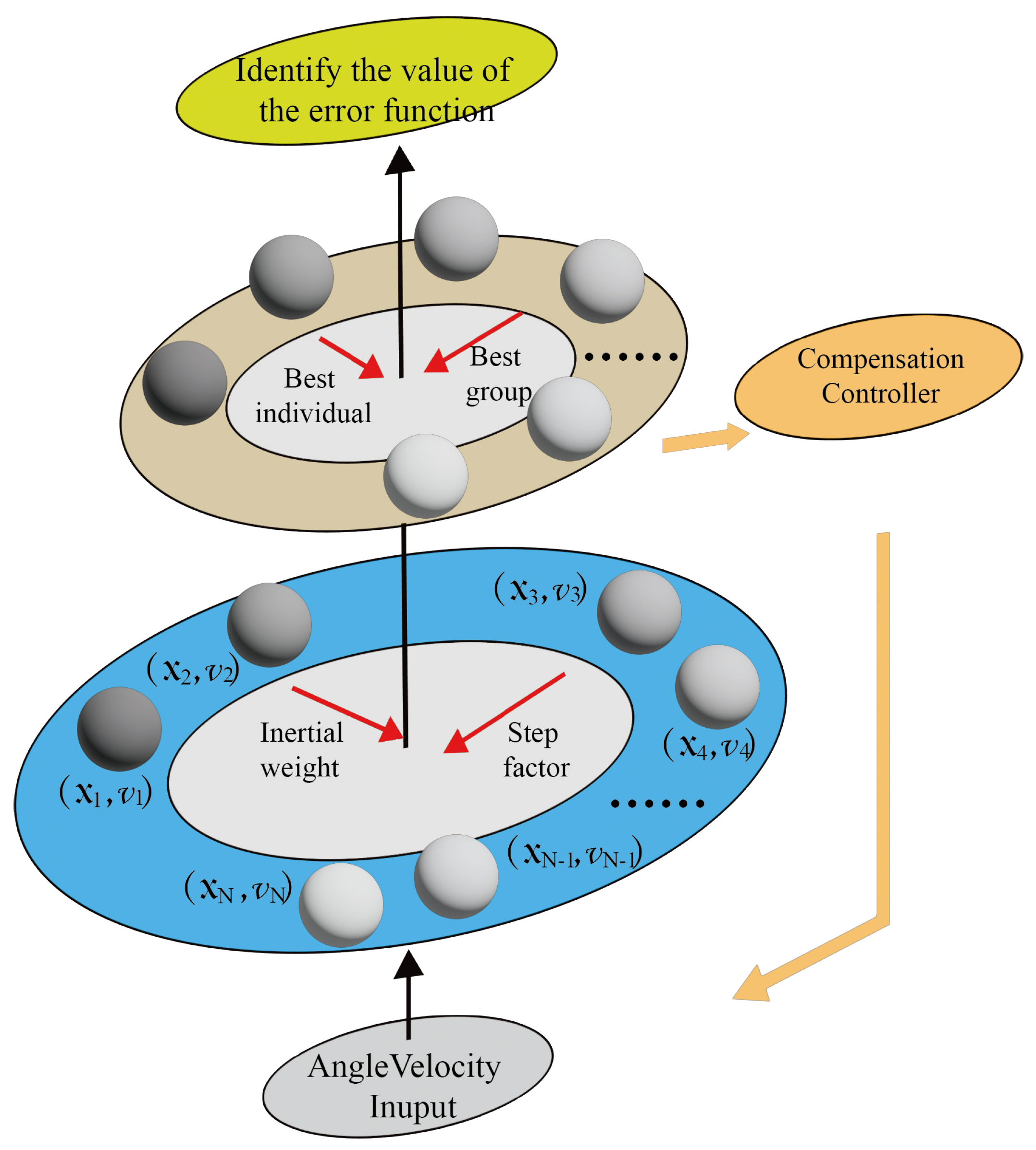
From the optimization theory, an intelligent identification algorithm is further used to identify the error parameters of the RIRG system. The PSO algorithm has the advantages of small computation, high accuracy, and fast convergence among many optimization algorithms. PSO is a swarm optimization algorithm inspired by the foraging process of flock birds, which is widely used to solve constraint optimization problems and find the optimal solution through simulating social behavior like cooperation and information sharing. The route decision of the flock while searching consists of three parts, spontaneous random search direction, its own searching experience, and the searching experience of the entire population. For the PSO algorithm, the foraging behavior of individual birds can be seen as the spontaneous random search of particles, and the optimal solution is the result of the optimal solution trend of the particle itself united with the best solution trend of the particle swarm. Each particle updates its properties of position and velocity according to the optimal fitness of itself and the optimal particle in the population so that the iteration direction of each particle is toward the region of the optimal solution.
The position of individual particles represents a trial solution for the search problem. The PSO is designed with time-varying inertia weights to enable it to consider the search performance, and its velocity and position update equations are as follows:
v i k + 1 = ω v i k + c 1 r 1 p i k X i k + c 2 r 2 p g k X i k X i k + 1 = X i k + v i k + 1
where p g k is the globally optimal particle and p i k is the locally optimal particle. v i k is the velocity attained by the particle after iterative search. X i k represents the position reached by the particle after iterative calculation. ω denotes the inertia weight. c 1 = 1.8 and c 2 = 2.5 are the learning factors of the particle and the population, respectively. r 1 and r 2 are the random search coefficient of the particle and the population, respectively.
Comparing the fitness of each particle with p i k , if the current value exceeds p i k , then the p i k value is set equal to the current location in the solution space. The fitness is compared with the best fitness observed previously in the overall population. If the current value exceeds p g k , then p g k is reset to the value of the current particle and the current particle position is recorded as the best solution.
(1)
Adaptive inertia weight
The traditional PSO algorithm has the disadvantage of poor balance between search and evolution. Since the inertia weight reflects the dependable degree of the particles on the previous update rate, the variable weight is more adaptive to the change in optimization requirements than the constant weight. At the beginning of the iteration, the search strategy focused on the search domain broadening to find as many local optimal solutions as possible. In order to locate the region where the potential globally optimal solution exists as soon as possible, the step size of each search by the particle is to be appropriately enlarged. In the later stages of the iteration, the population requires search property for precise localization in the range of existing optimal solutions. Therefore, the search step size should be appropriately reduced. In addition, the process of random movement and then precise localization of the particle population is not a linear transition, so linearly varying inertia weight is unable to respond to changes in individual learning rates. To meet the tasks of these two search phases, nonlinear inertia weights are introduced to adapt to this situation. The adaptive weights are calculated as
ω t = ω m ω c ω m 1 1 1 + t t T T 1 + t t T T
where ω c and ω m denote the minimum inertia weight and maximum weight of particles when the population is initialized. ω c usually takes 0.1 and ω m usually takes 0.9, t is the current number of iterations, and T is the utmost number of iterations.
(2)
IPSO based on chaotic variables
The diversity of population particles represents searching accuracy and convergence precision. If the distribution of initial values is too narrow, it may lead to a lack of diversity in the early population and affect the global search ability. There is a need for greater initial distribution diversity to mitigate the effects of uneven individual distribution during the population iteration. Benefiting from the stochastic and ergodic characteristics, the chaos technology has the ability out of the local optimal solution to overcome the defect of the PSO algorithm that is easy to fall into the local extreme point and thus has better performance of global optimization. To obtain a stronger chaotic traversal, we choose the Cubic chaotic mapping which is constructed by raising the degree of Logistic mapping. the Cubic chaotic mapping is appropriate and defined by the following equation:
λ i + 1 = ε λ i 1 λ i 2
where ε = 2.595 for an unimodal surjection and ergodic enough in the range 0 , 1 [26].
The Cubic chaotic mapping is used to design the initial search speed and position of particles for improving the uniformity of particle distribution:
X i k = β i k X max X min + X min
v i k = α i k v max v min + v min
where α i k and β i k are generated by Cubic chaos mapping.
Figure 5 is the flowchart of the IPSO. The process of parameter identification is to inversely obtain the corresponding model parameters from the measurement output so that the simulation result under those parameters can be as close as possible to the actual measured response curve. The optimization function is introduced as the IPSO algorithm fitness function to obtain the optimization parameters. Therefore, the parameter identification problem can be transformed into a set of optimization problems. Based on a set of optimal parameter vectors, the error between the simulation response result and the actual measurement reaches the minimum thus obtaining the identification result of error parameters. The target function is established according to the minimum sum of squares of errors, as shown in Equation (22):
J = i = 1 N 1 2 θ ˙ i ˙ ^ θ i T θ ˙ i ˙ ^ θ i
The harmonic parameters are evaluated using the IPSO, and the optimal solution is obtained. Each particle represents a different set of vector u and these particles are conceptual entities that travel through the multidimensional search space. At any iteration, each particle has a position and a velocity. The identification error function is designed to evaluate the compensation model performance. The identification error function is also the objective function of the particle swarm update, which ultimately reflects the accuracy of the identification. Then, the intelligent controller compares the gyroscope output with the fitting angular output by identification and updates the parameter vector by using the IPSO method. The individuals with the smallest fitness function are found by following the current search best value. When the minimum of the function is reached, the RIRG output is decomposed optimally.

5. Simulation Results and Performance Evaluation

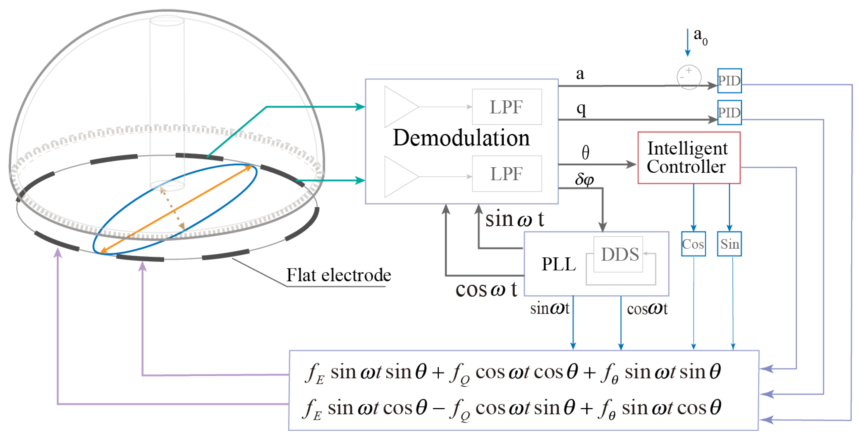
In order to validate the effectiveness and accuracy of error compensation using the IPSO parameter identification method, a series of tests were conducted on a self-built simulated dynamic system. The simulation validation system is shown in Figure 6.
The proposed parameter identification method is validated through a comprehensive numerical simulation of the RIRG system, which incorporates the dynamics model of the gyroscope, the phase-locked loop for resonance tracking, the energy compensation loop for amplitude maintenance, and the motion feedback for quadrature nulling. The training set for the prediction model is constructed using the output of standing wave pattern angle simulations and the corresponding angular velocity input data. The performance of error parameters identification and compensation was compared based on LSM, PSO, and IPSO methods. The parameters used in the simulation related to the real RIRG device are presented in Table 1.
The LSM-based parameter identification process is shown in Figure 7. The forgetting factor is chosen to be 0.92 to improve the tracking accuracy and the damping factor is 0.9 to adapt to the nonlinearity of the system. Since the initial value of LSM is selected blindly, the estimation error jumps drastically in the early stage of identification, and as the number of measurements increases, the unreliability of the initial value gradually disappears, and the identification result tends to be stable. In addition to the problem of insufficient accuracy, LSM has the disadvantage of not being able to be implemented in real-time systems, where it cannot dynamically identify the error parameters based on the current error and system state to achieve optimal compensation.
The core of the IPSO algorithm is to find a particle’s position that can satisfy the population’s optimal solution, and the investigation index is the objective function value as small as possible. The range of particle motion velocity is set within 1 , 1 and the range of u is set within 1 , 1 
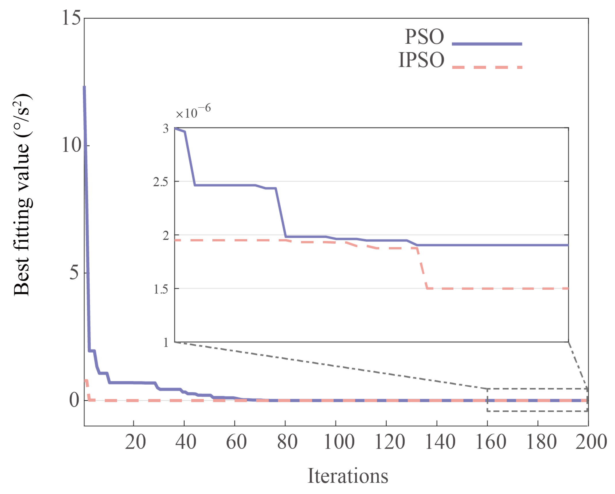
, the population particle number is set as 150 and the number of iterations is set as 200. And then, the PSO and IPSO parameter initialization are set, respectively, to generate the random population. As shown in Figure 8, the individuals with the smallest fitness function are found through iterations in the population. When the number of iterations reaches 160, the IPSO algorithm has converged, while the PSO has not yet fully converged.
The stability and the optimal rate of convergence of the PSO and IPSO are shown in Figure 9, which means the number of iterations required to reach the optimal solution is reduced. This can be a critical factor in real-time system implementation where computational efficiency is important. By visualizing the optimization performance of the two algorithms under the same conditions, it can be intuitively seen that IPSO outperforms PSO in terms of convergence speed and global search capability.
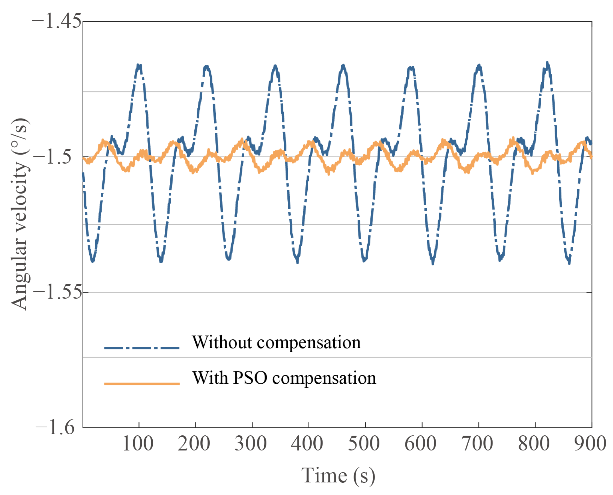
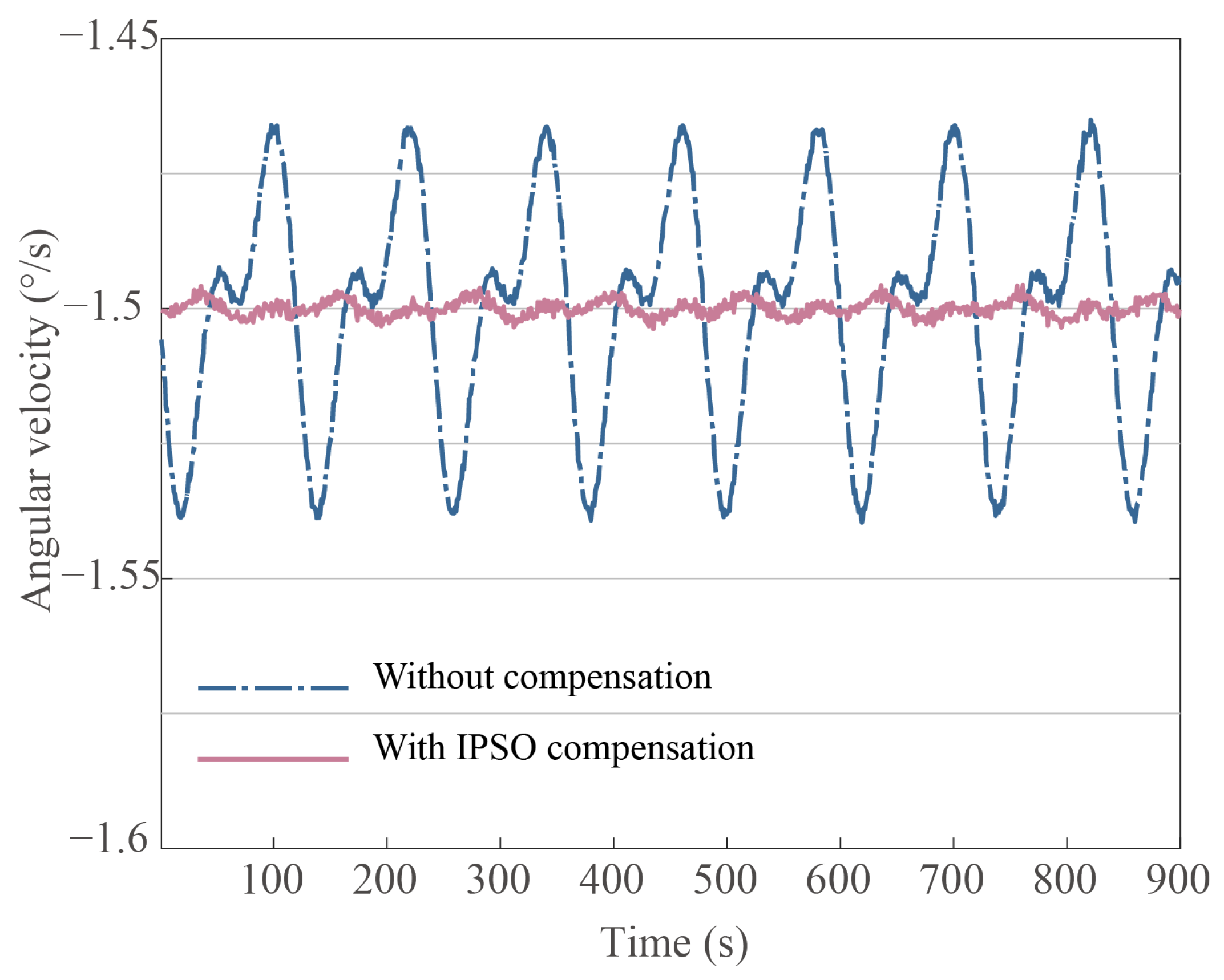
The error parameter identification and compensation experiments were conducted to verify the identification model’s effectiveness and the identification method’s feasibility. This paper analyzes and simulates gyroscope bias drift compensation under three identification methods with a standard deviation of 1 × 10⁻⁵ sampling noise added to the simulation model. The results from the IPSO-based parameter identification were successfully used in the feedback control to minimize angle drift error. Other methods were used for the comparison to prove the effectiveness, including LSM and PSO.
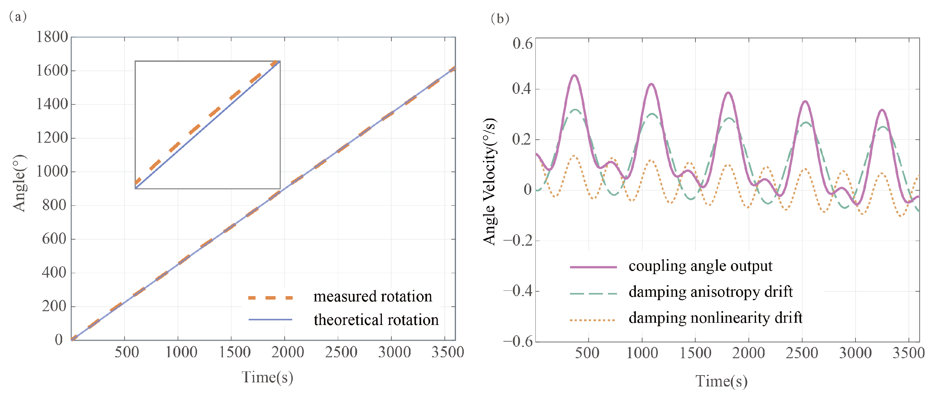
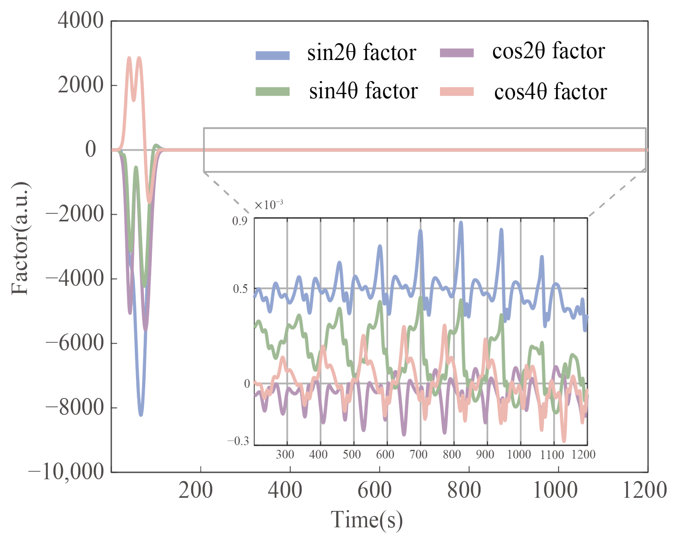
When the gyroscope is under constant rate input, the fluctuation magnitude of the standing wave rotation rate indicates the maximum angle drift. Figure 9, Figure 10 and Figure 11 show the compensation results after minimizing the harmonic errors under diverse parameter identification methods and demonstrates the effectiveness of the IPSO as a powerful tool in the process of reducing bias drift error caused by damping anisotropy and damping nonlinearity. In Figure 9, Figure 10 and Figure 11, the input rate condition is kept consistent. Following the IPSO-based compensation, the bias drift decreased from 2.1046 × 10 2 °/s to 1.4722 × 10 3 °/s. In comparison, other identification methods, including the traditional PSO and LSM, bias drift compensated values of 2.4533 × 10 3 °/s and 9.8372 × 10 3 °/s, respectively.
The standard deviations and the mean of measurements based on LSM, PSO, and IPSO identification are summarized in Table 2. It can be seen that the LSM is lower than the intelligent algorithm in terms of recognition accuracy, the PSO has improved recognition accuracy but has a lower convergence rate, and the error compensation results using the improved PSO intelligent algorithm are much better than the other two algorithms.
In summary, the nonlinear error analysis and compensation method proposed in this paper can be successfully applied to RIRG and achieve high accuracy identification and compensation of the error parameters.

6. Conclusions

This paper presents a novel method for achieving high-precision identification and compensation of bias drift in RIRG dynamic output, which establishes the relationship between standing wave pattern angle and RIRG harmonic errors by introducing a nonlinearity component. Initially, the RIRG nonlinear error model reveals the propagation of damping-dependent elements in the RIRG system, including damping anisotropy error and damping nonlinearity error, leading to threshold regions, distortions, and periodic vibrations in measurements. Subsequently, a model for identifying harmonic parameters, which considers both damping anisotropy and nonlinear errors, is developed based on the dynamic drift model of the RIRG. Parameter identification of RIRG is an essential prerequisite for any adaptive control and state feedback compensation to minimize output errors. An IPSO method based on the slow varying averaged dynamic model is applied to harmonic error parameter identification in this paper. With the help of adaptive inertia weight and a richer initial distribution diversity of the population through chaos-based technique, it leads to IPSO for RIRG identification with improved accuracy, stability, and suitability. Compared with the LSM-based method and PSO-based identification methods, the measurement accuracy and the effect of harmonic components compensation are significantly enhanced. Numeric simulation validates the proposed algorithms with fast convergence and great accuracy. Estimated nonlinear damping parameters from the IPSO are effectively used for setting the correct amount of feedback to compensate for the nonlinear error in the angular drift. Based on the identification result, the compensation for the RIRG dynamic output error is realized. The dynamic experiment verifies the effectiveness of the proposed method, and the bias drift of the RIRG dynamic is reduced from 2.1046 × 10 3 °/s to 1.4722 × 10 3 °/s, the bias drift error is reduced by 93%, and accuracy is improved by an order of magnitude.

Author Contributions

This paper was accomplished by all the authors. Conceptualization, X.Y. and G.Y.; methodology, X.Y. and Y.T.; software, X.Y.; validation, X.Y. and Y.T.; formal analysis, X.Y. and Y.T.; investigation, X.Y.; resources, G.Y. and Q.C.; data curation, X.Y.; writing—original draft preparation, X.Y.; writing—review and editing, X.Y.; visualization, X.Y. and Y.T.; project administration, G.Y. and Y.T.; funding acquisition, G.Y. and Q.C. All authors have read and agreed to the published version of the manuscript.

Funding

This work was supported by the National Key R&D Program of China under Grant No. 2021YFB3201504.

Data Availability Statement

The data are not publicly available due to privacy.

Conflicts of Interest

The authors declare no conflicts of interest.

References

  1. Jeanroy, A.; Grosset, G.; Goudon, J.C.; Delhaye, F. HRG by Sagem from laboratory to mass production. In Proceedings of the 2016 IEEE International Symposium on Inertial Sensors and Systems, Seattle, WA, USA, 30 November–1 December 2016; pp. 1–4. [Google Scholar] [CrossRef]
  2. Perelyaev, S.; Bodunov, S.; Zhuravlev, V.; Bodunov, B.P. New Gyroscopes of the “Generalized Foucault Pendulum” Family: Some Fundamental Issues of Theory and Applied Aspects of Its Implementation in the Engineering Practice of Modern Gyroscopy. In Proceedings of the 2020 27th Saint Petersburg International Conference on Integrated Navigation Systems (ICINS), Saint Petersburg, Russia, 25–27 May 2020; pp. 1–11. [Google Scholar] [CrossRef]
  3. Shatalov, M.Y.; Joubert, S.V.; Coetzee, C.E. The influence of mass imperfections on the evolution of standing waves in slowly rotating spherical bodies. J. Sound Vib. 2011, 330, 127–135. [Google Scholar] [CrossRef]
  4. Prikhodko, I.P.; Gregory, J.A.; Bugrov, D.I.; Judy, M.W. Overcoming limitations of Rate Integrating Gyroscopes by virtual rotation. In Proceedings of the 2016 IEEE International Symposium on Inertial Sensors and Systems, Seattle, WA, USA, 30 November–1 December 2016; pp. 5–8. [Google Scholar] [CrossRef]
  5. Prikhodko, I.P.; Gregory, J.A.; Judy, M.W. Virtually rotated MEMS gyroscope with angle output. In Proceedings of the 2017 IEEE 30th International Conference on Micro Electro Mechanical Systems (MEMS), Las Vegas, NV, USA, 22–26 January 2017; pp. 323–326. [Google Scholar] [CrossRef]
  6. Apostolyuk, V. Whole angle force rebalance control for coriolis vibratory gyroscopes. In Proceedings of the 2014 IEEE 3rd International Conference on Methods and Systems of Navigation and Motion Control (MSNMC), Kiev, Ukraine, 14–17 October 2014; pp. 59–61. [Google Scholar] [CrossRef]
  7. Gando, R.; Maeda, S.; Masunishi, K.; Tomizawa, Y.; Ogawa, E.; Hatakeyama, Y.; Itakura, T.; Ikehashi, T. A MEMS rate integrating gyroscope based on catch-and-release mechanism for low-noise continuous angle measurement. In Proceedings of the 2018 IEEE Micro Electro Mechanical Systems (MEMS), Belfast, UK, 21–25 January 2018; pp. 944–947. [Google Scholar] [CrossRef]
  8. Guo, K.; Wu, Y.; Zhang, Y.; Xiao, D.; Wu, X. Adaptive compensation of damping asymmetry in whole-angle hemispherical resonator gyroscope. AIP Adv. 2020, 10, 105109. [Google Scholar] [CrossRef]
  9. Liu, J.; Yang, Y.; Guo, S.; Fan, B.; Xuan, L.; Bu, F.; Xu, D. A Novel Compensation Method for Eliminating Precession Angular-Rate Bias in MEMS Rate-Integrating Gyroscopes. IEEE Access 2020, 8, 145611–145619. [Google Scholar] [CrossRef]
  10. Zargari, S.; Moezzi, M. A New Readout Circuit with Robust Quadrature Error Compensation for MEMS Vibratory Gyroscopes. Circuits Syst. Signal Process. 2022, 41, 3050–3065. [Google Scholar] [CrossRef]
  11. Taheri-Tehrani, P.; Challoner, A.D.; Horsley, D.A. Micromechanical Rate Integrating Gyroscope with Angle-Dependent Bias Compensation Using a Self-Precession Method. IEEE Sens. J. 2018, 18, 3533–3543. [Google Scholar] [CrossRef]
  12. Ruan, Z.; Ding, X.; Pu, Y.; Gao, Y.; Li, H. In-Run Automatic Mode-Matching of Whole-Angle Micro-Hemispherical Resonator Gyroscope Based on Standing Wave Self-Precession. IEEE Sens. J. 2022, 22, 13945–13957. [Google Scholar] [CrossRef]
  13. Tsukamoto, T.; Tanaka, S. Rate Integrating Gyroscope Using Independently Controlled CW and CCW Modes on Single Resonator. J. Microelectromech. Syst. 2021, 30, 15–23. [Google Scholar] [CrossRef]
  14. Yan, K.; Wang, X.; Zou, K.; Zhang, X.; Qu, T.; Che, C.; Lu, Q. Self-Excitation Enabled Decoupling, Calibration, and Compensation of Errors for Whole-Angle Hemispherical Resonator Gyroscope. IEEE Trans. Instrum. Meas. 2024, 73, 1001613. [Google Scholar] [CrossRef]
  15. Yi, X.; Yang, G.; Cai, Q.; Cheng, R.; Tu, Y.; Wang, Y.; Song, N. A Novel Self-Modulation Method for Whole-Angle Resonator Gyroscope Based on High Harmonic Compensation. IEEE Sens. J. 2024, 24, 31827–31836. [Google Scholar] [CrossRef]
  16. Nitzan, S.H.; Taheri-Tehrani, P.; Defoort, M.; Sonmezoglu, S.; Horsley, D.A. Countering the Effects of Nonlinearity in Rate-Integrating Gyroscopes. IEEE Sens. J. 2016, 16, 3556–3563. [Google Scholar] [CrossRef]
  17. Taheri-Tehrani, P.; Defoort, M.; Horsley, D.A. Operation of a high quality-factor gyroscope in electromechanical nonlinearities regime. J. Micromech. Microeng. 2017, 27, 075015. [Google Scholar] [CrossRef]
  18. Zaitsev, S.; Shtempluck, O.; Buks, E.; Gottlieb, O. Nonlinear damping in a micromechanical oscillator. Nonlinear Dyn. 2012, 67, 859–883. [Google Scholar] [CrossRef]
  19. Polunin, P.M.; Yang, Y.; Dykman, M.I.; Kenny, T.W.; Shaw, S.W. Characterization of MEMS Resonator Nonlinearities Using the Ringdown Response. J. Microelectromech. Syst. 2016, 25, 297–303. [Google Scholar] [CrossRef]
  20. Hu, Z.; Gallacher, B.J. Effects of Nonlinearity on the Angular Drift Error of an Electrostatic MEMS Rate Integrating Gyroscope. IEEE Sens. J. 2019, 19, 10271–10280. [Google Scholar] [CrossRef]
  21. Vatanparvar, D.; Shkel, A.M. Rate-Integrating Gyroscope Operation in The Non-Linear Regime. In Proceedings of the 2022 DGON Inertial Sensors and Systems (ISS), Braunschweig, Germany, 13–14 September 2022; pp. 1–18. [Google Scholar] [CrossRef]
  22. Xia, D.; Kong, L.; Hu, Y.; Ni, P. Silicon microgyroscope temperature prediction and control system based on BP neural network and Fuzzy-PID control method. Meas. Sci. Technol. 2015, 26, 025101. [Google Scholar] [CrossRef]
  23. Yu, H.; Jin, X.; Liu, X.H.; Liu, D.P.; Li, Z.X.; Li, S.L.; Duan, J.; Zhang, J.C.; Li, C.J. Pose error identification algorithm based on hemispherical resonant gyroscope assembly capacitance uniformity. Measurement 2022, 198, 198. [Google Scholar] [CrossRef]
  24. Li, Y.X.; Xi, B.Q.; Ren, S.Q.; Wang, C.H. Precision Enhancement by Compensation of Hemispherical Resonator Gyroscope Dynamic Output Errors. IEEE Trans. Instrum. Meas. 2023, 72, 2516510. [Google Scholar] [CrossRef]
  25. Ren, L.; Wang, D.; Yan, X.; Zhang, Y.; Wang, J. A Novel Chaotic Particle Swarm Optimized Backpropagation Neural Network PID Controller for Four-Switch Buck-Boost Converters. Actuators 2024, 13, 464. [Google Scholar] [CrossRef]
  26. Sarmah, H.; Das, M. Various bifurcations in a cubic map. Int. J. Adv. Sci. Tech. Res. 2014, 4, 827–846. [Google Scholar]
Figure 1. Amplitude–frequency characteristic curves of the resonator at different excitation force.
Actuators 14 00068 g001
Figure 2. (a) Vibration mode of the RIRG, (b) working principle of the RIRG.
Actuators 14 00068 g002
Figure 3. There are two types of threshold−restricted phenomena depending on the magnitude of external input. Results for (a) total restricted threshold where the RIRG locks to a certain angle and (b) partial restricted threshold where the RIRG appears as a false threshold region.
Actuators 14 00068 g003
Figure 4. (a) Comparison of the theoretical angular measurement value and the actual angular measurement with drifts fluctuating around the theoretical output. (b) There are harmonic forms of the angular measurement drift errors in the angular velocity.
Actuators 14 00068 g004
Figure 5. IPSO algorithm flowchart.
Actuators 14 00068 g005
Figure 6. Block diagram of the electronics and the control loops.
Actuators 14 00068 g006
Figure 7. Parameter identification convergence process based on LSM.
Actuators 14 00068 g007
Figure 8. Convergence process of error discrimination function based on PSO and IPSO algorithms.
Actuators 14 00068 g008
Figure 9. Simulation results before and after nonlinear error compensation based on LSM identification.
Actuators 14 00068 g009
Figure 10. Simulation results before and after nonlinear error compensation based on PSO identification.
Actuators 14 00068 g010
Figure 11. Simulation results before and after nonlinear error compensation based on IPSO identification.
Actuators 14 00068 g011
Table 1. RIRG structure and electrical parameters.
SymbolParameterValue
ω resonance frequency6800 Hz
Δ ω frequency mismatch0.001 Hz
τ time constant348 s
mequivalent mass2.5 g
V D C DC voltage100 V
delectrode gap80 μm
C 0 nominal capacitance2.45 pF
x x d d amplitude–gap ratio 0.1
Ω angular velocity input5°/s
β control gain60
Adetection gain1 V/μm
Table 2. Compensation performance summary of diverse identification methods.
MethodBefore CompensationLSMPSOIPSO
MAE 1.4996 1.4998 1.4999 1.5000
RMSE2.1046 × 10 2 9.8372 × 10 3 2.4533 × 10 3 1.4722 × 10 3
Disclaimer/Publisher’s Note: The statements, opinions and data contained in all publications are solely those of the individual author(s) and contributor(s) and not of MDPI and/or the editor(s). MDPI and/or the editor(s) disclaim responsibility for any injury to people or property resulting from any ideas, methods, instructions or products referred to in the content.

