Encouraging Guidance: Floating Target Tracking Technology for Airborne Robotic Arm Based on Reinforcement Learning

 , , ,
, , ,
Abstract
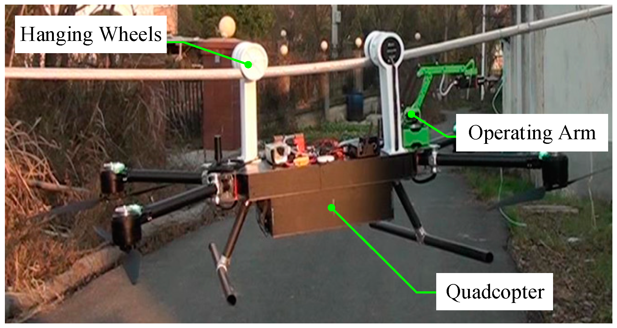
1. Introduction
2. Algorithm Principles and Processes
2.1. ARA Status Description
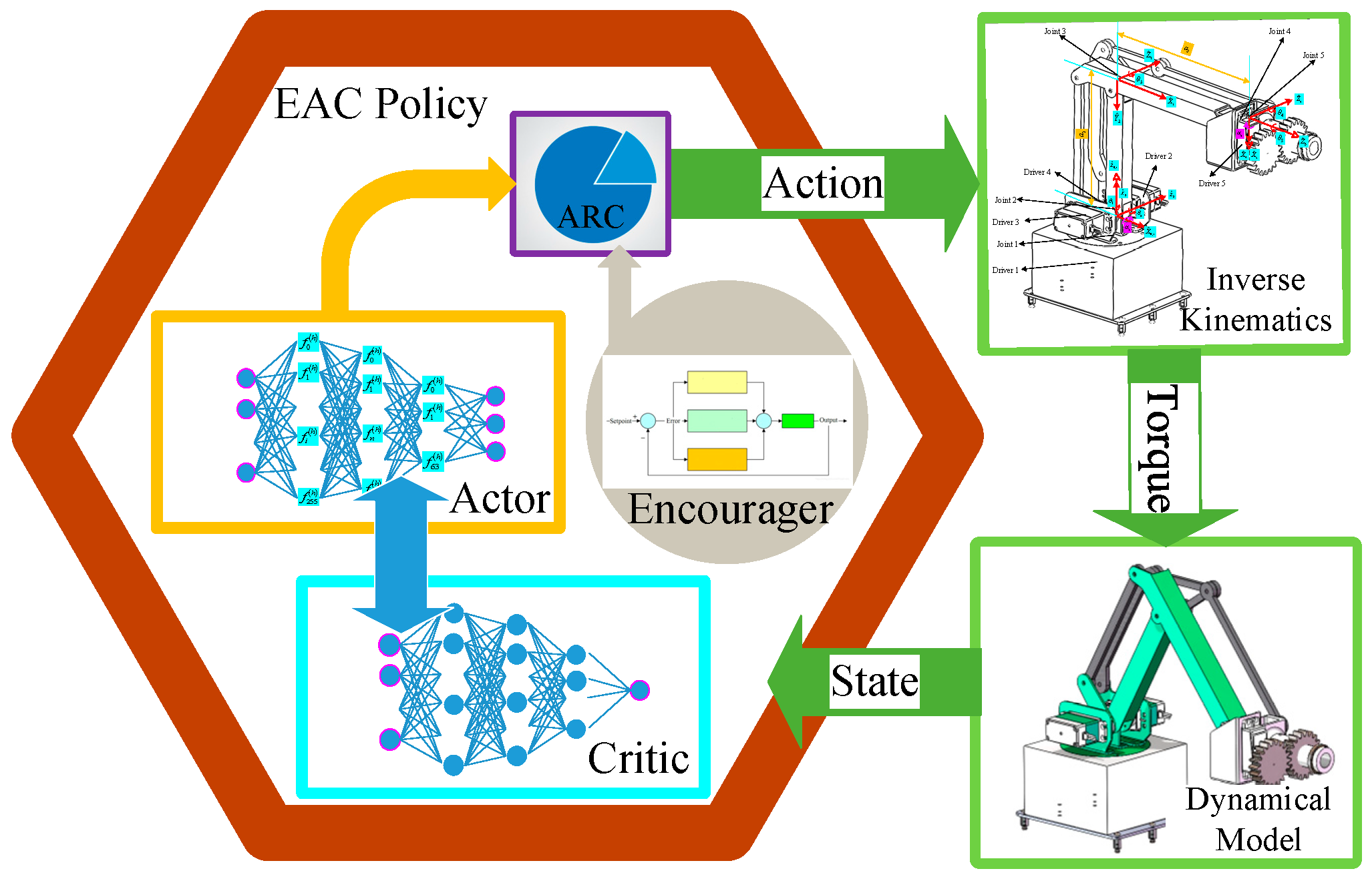
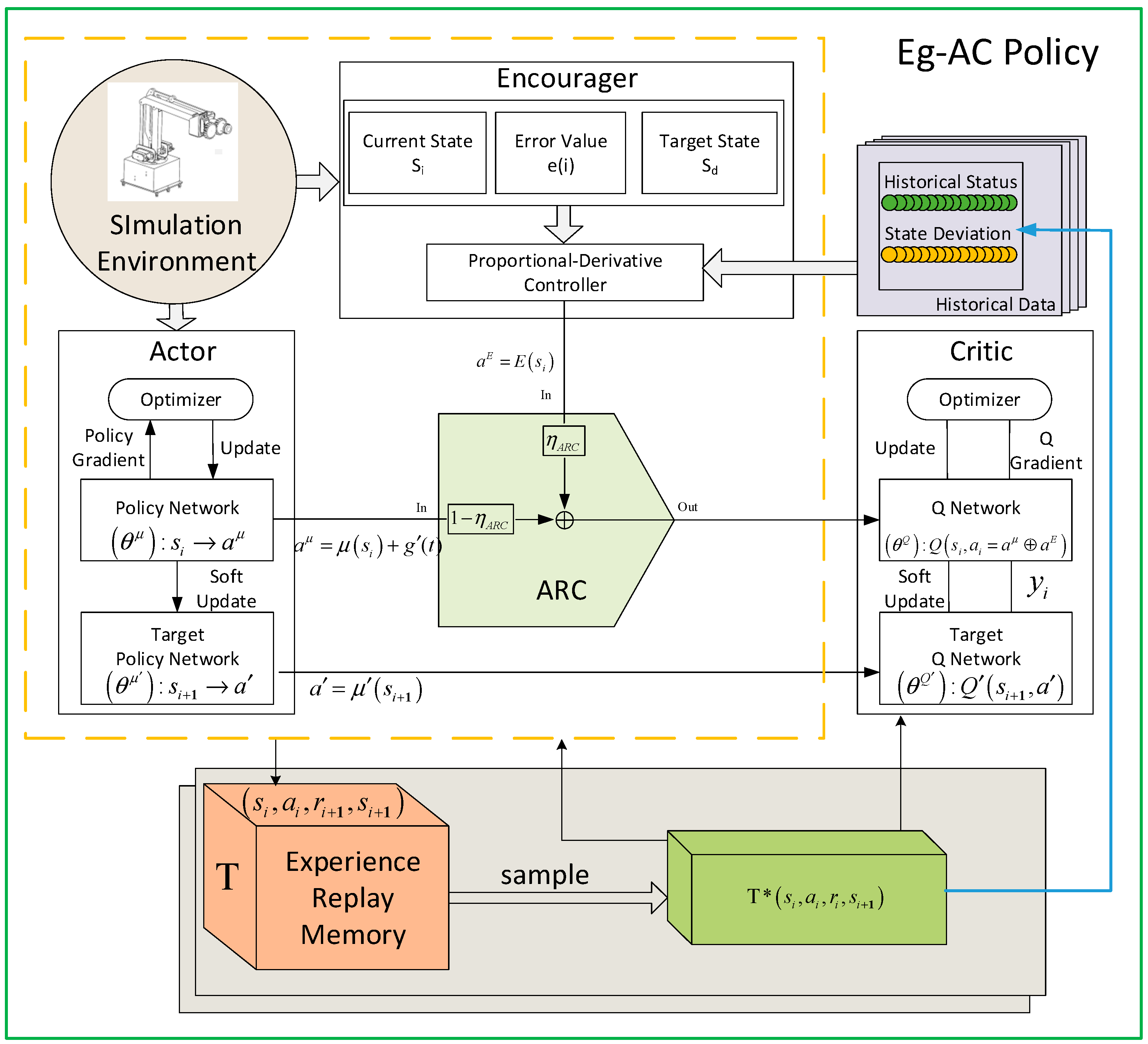
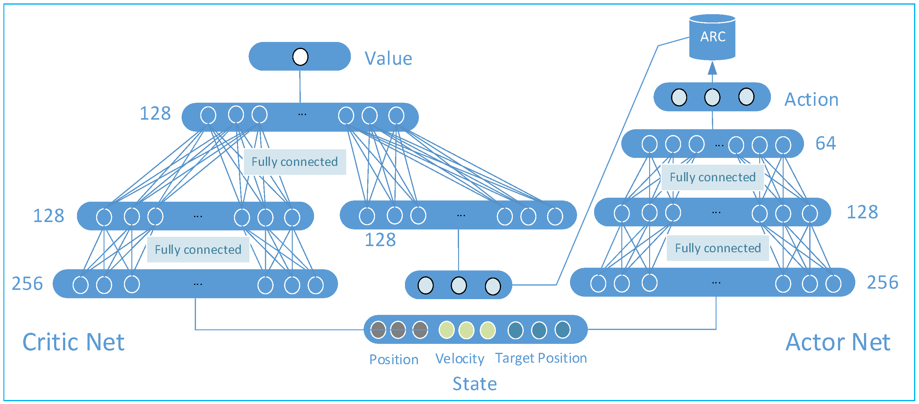
2.2. Eg-ac Control Policy
- (a)
- ARC Module
- (b)
- HRLP Reward Mechanism
| Algorithm 1: Eg-ac Algorithm |
by Equation (12) initialize the experience cache space T for episode from 1 to Limit do Initialize a noise function receive the initial state for t = 1 to do , store in T sample a batch of random in T, where set target value function via Equation (6) update critic by minimizing the loss via Equation (7) update actor policy by policy gradient via Equations (8) and (9) update networks via Equations (10) and (11) end for end for |
3. Preparation Work for Simulation
3.1. Establishment of ARA Mathematical Model
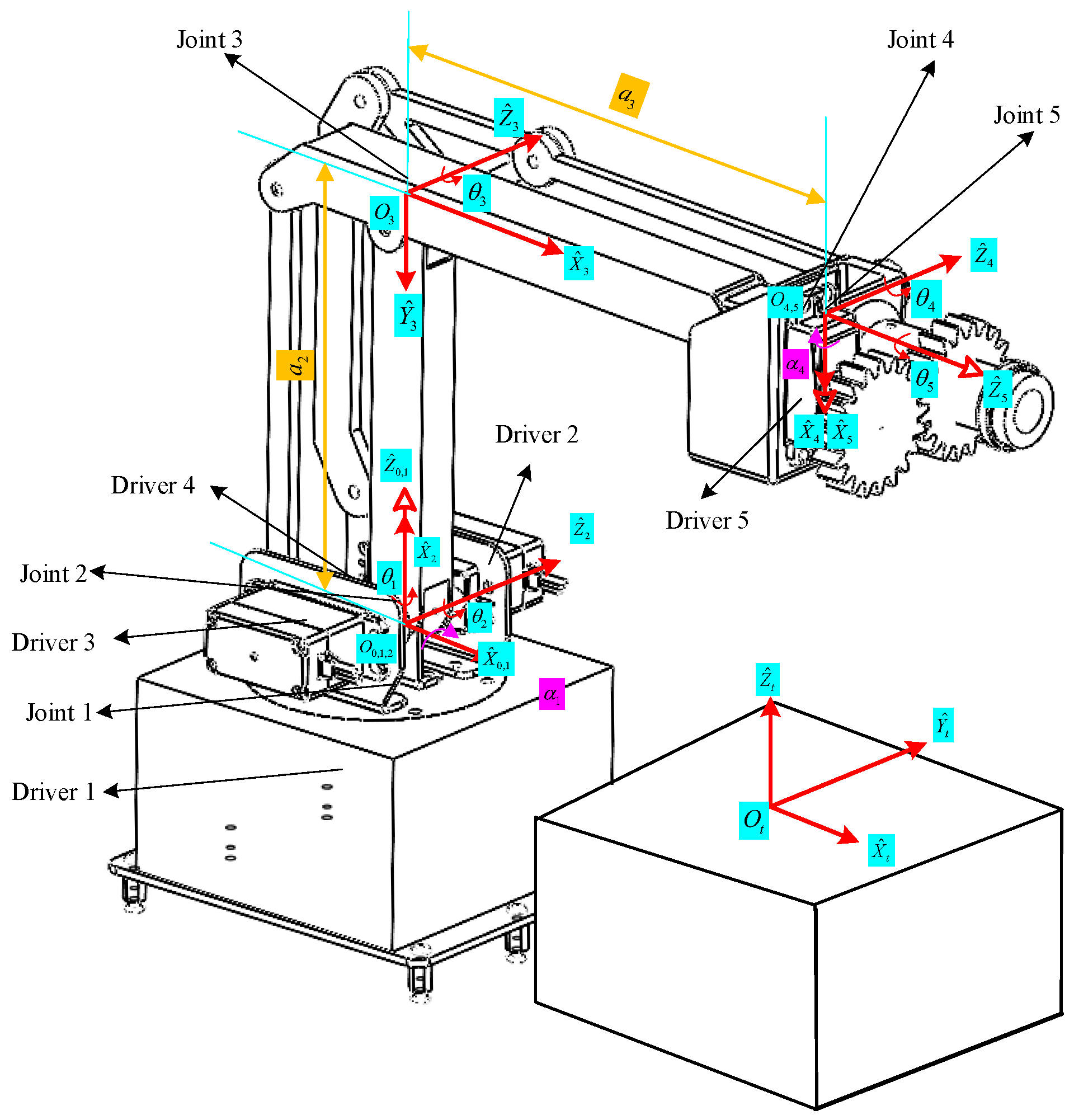
3.1.1. ARA Kinematic Analysis
3.1.2. ARA Dynamic Analysis
3.2. Network Architecture Design
- (1)
- The definition of the reward value is the negative value of the distance between the end of the ARA and the target position, which means that the larger the error, the lower the reward value.
- (2)
- Each training batch is executed times. When there is an error between the end of the ARA task and the target position during an experience, the task is considered completed, and the current experience is stopped and reset to enter the next experience.
- (3)
- Let the simulation time step be and the total training steps be .
- (4)
- Set learning rates , , and batch sampling quantity .
- (5)
- Controller parameters in the encourager: .
- (6)
- Output range setting: , , .
- (7)
- Set the random noise range to .
- (8)
- The size of the ARA connecting rod is .
- (9)
- To ensure that the pitch and roll angles of the ARA end remain unchanged, and to make the end face of joint 5 perpendicular to the plane of the operating arm, the following settings are used: , .
- (10)
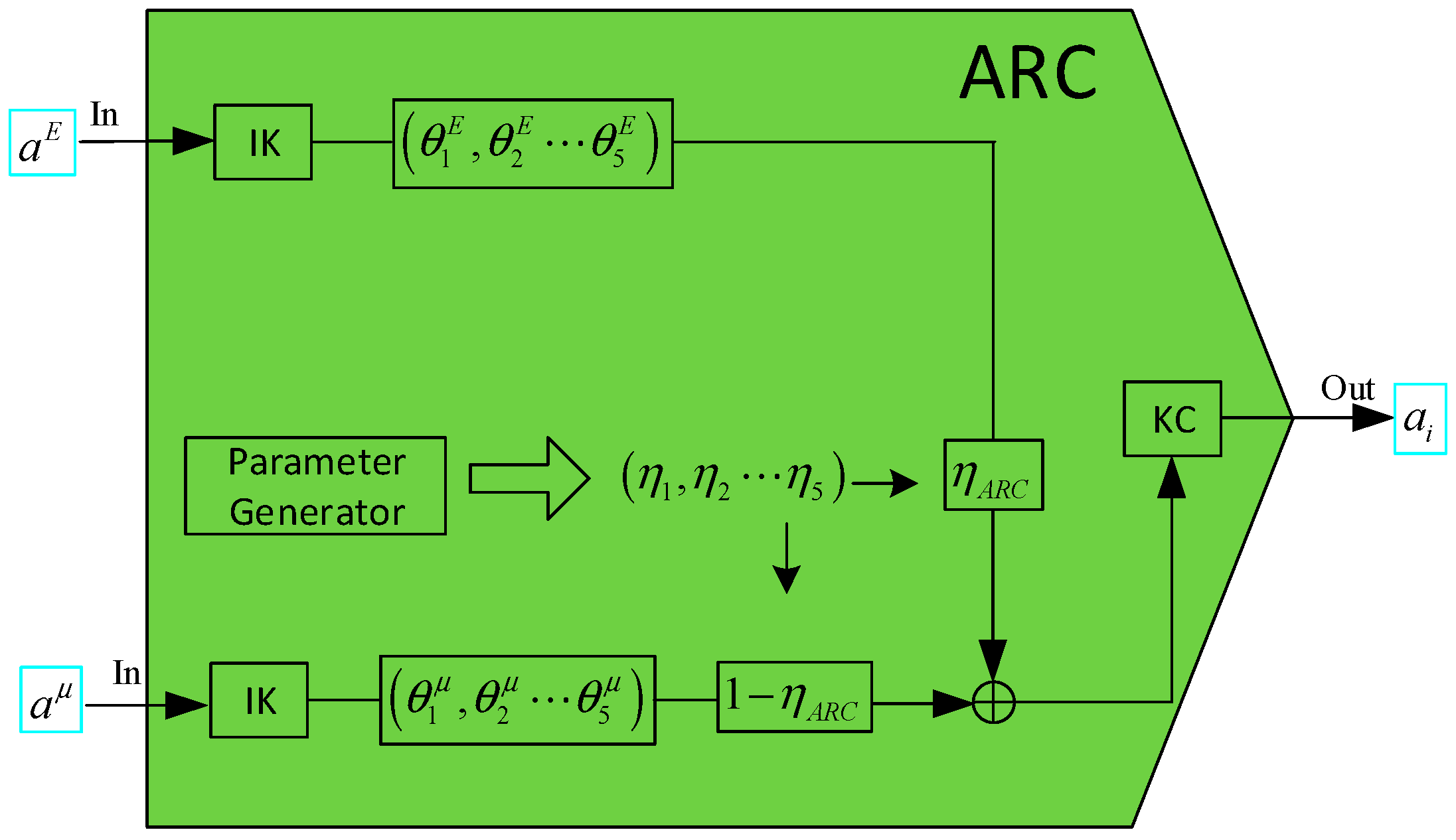
- The adoption rate parameter of the ARC is composed of a set of random numbers with five elements generated by the computer. The process diagram is shown in Figure 6. In this process, the input variables are first subjected to inverse kinematics (IK) to obtain the joint positions of the ARA and then integrated into through adoption rate calculation. Finally, the final behavior is output through kinematic calculations (KCs). Among them, . Set when the training steps are .
- (11)
- The simulated computer configuration used an Intel(R) Core (TM) i5-7300HQ (ASUS, Taipei, China).
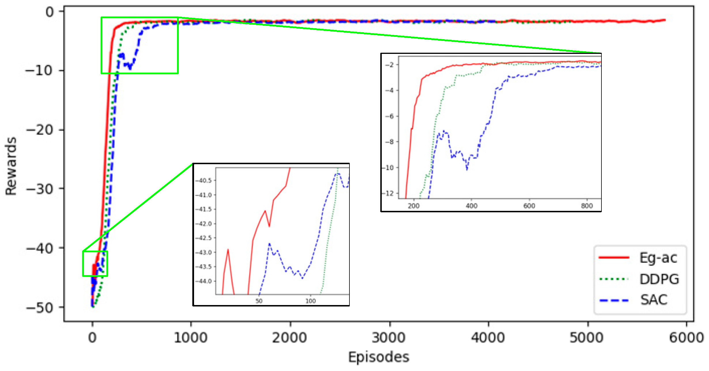
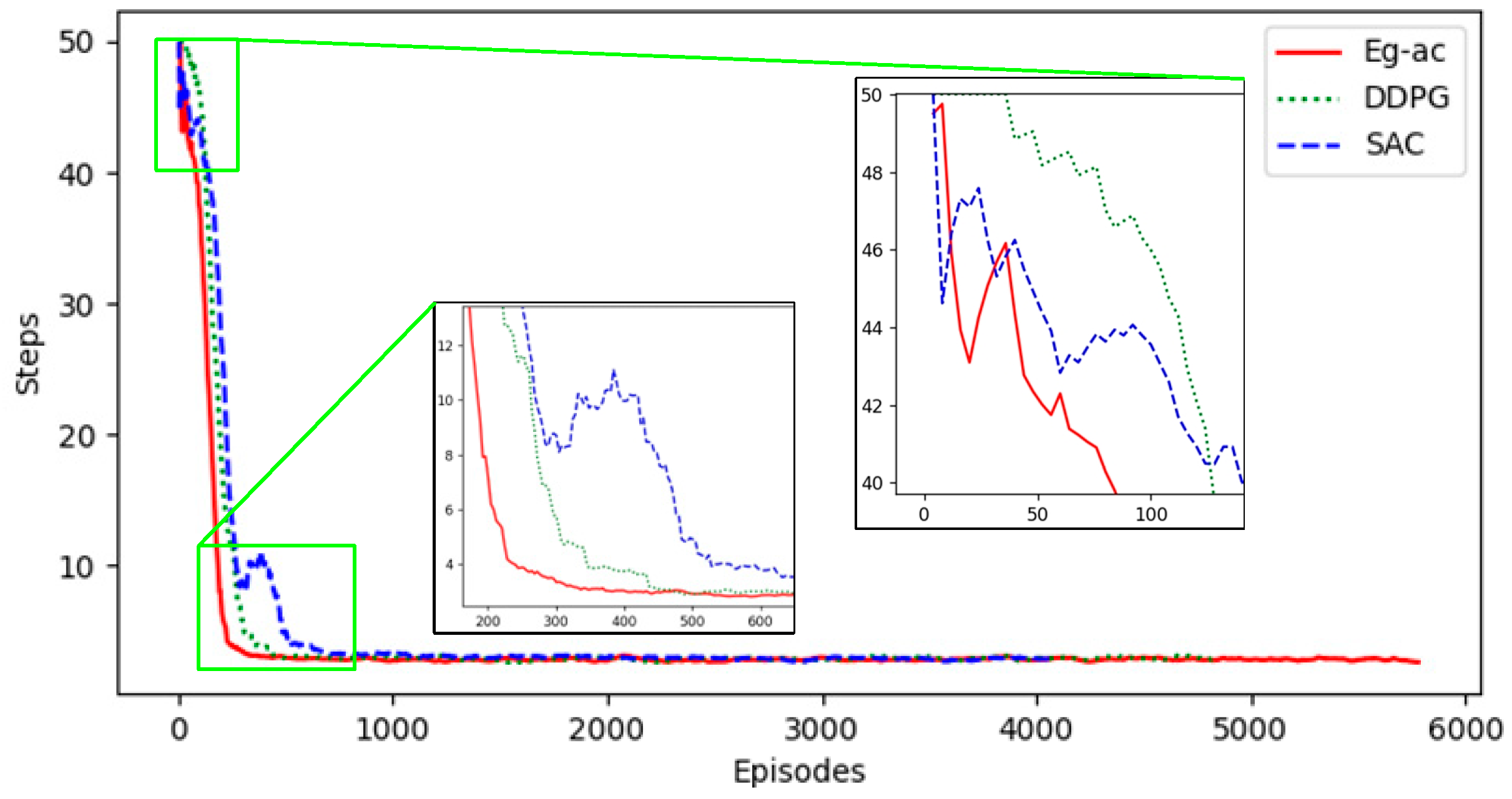
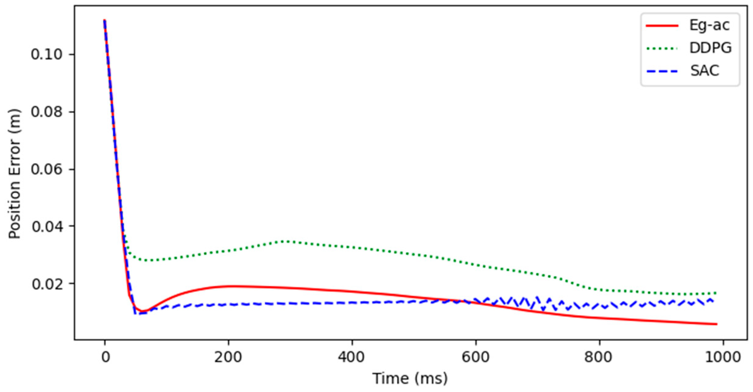
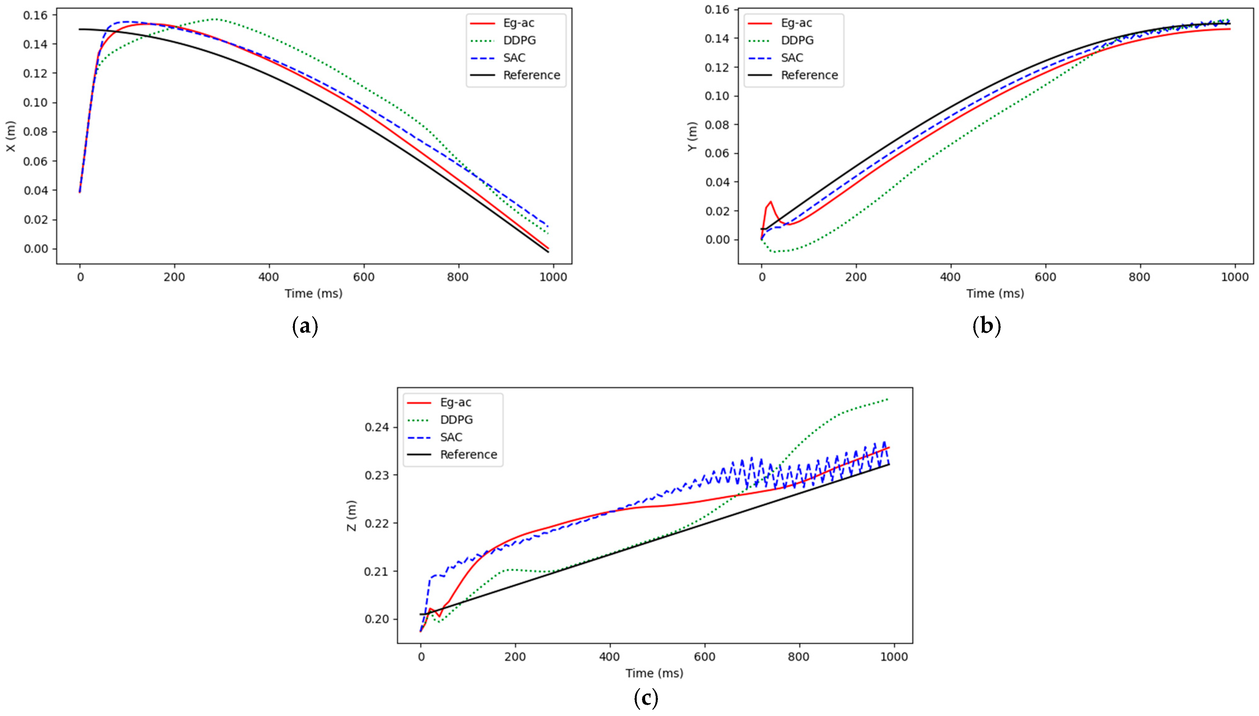
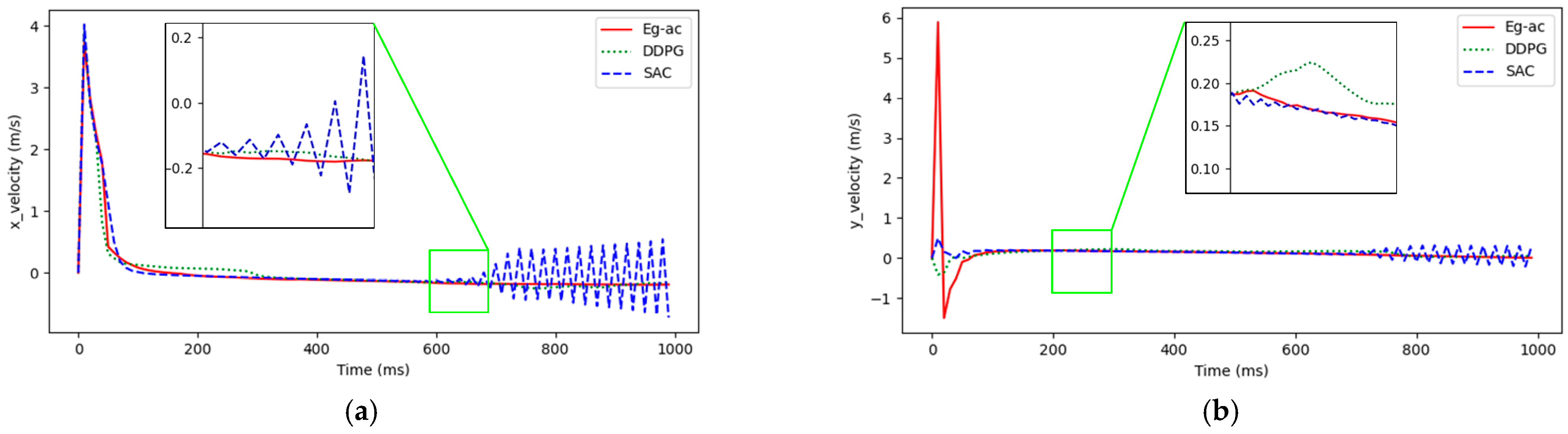
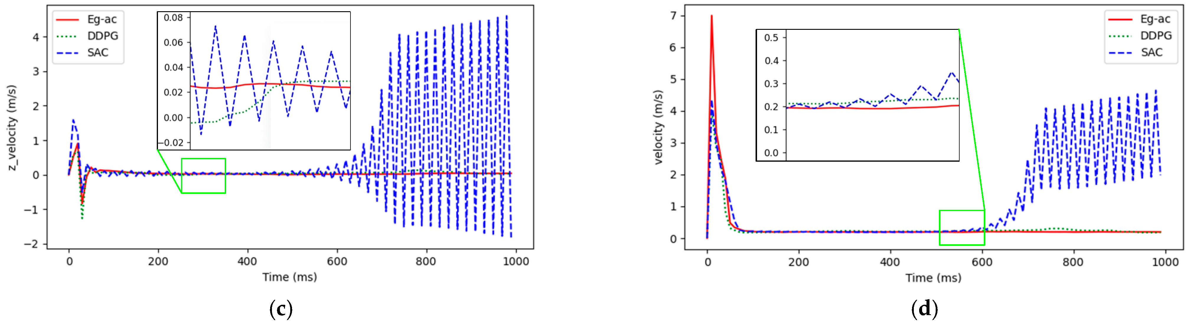
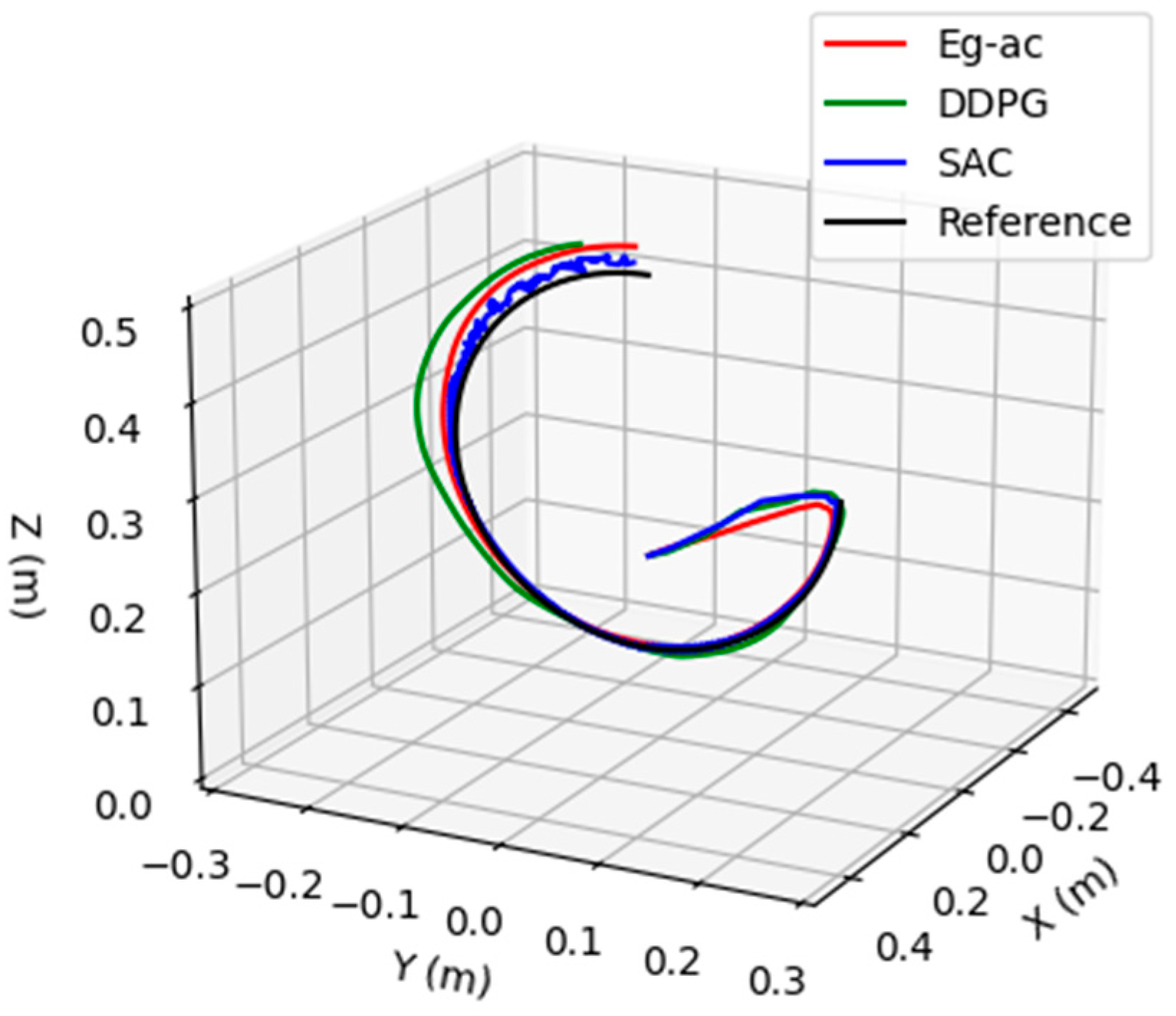
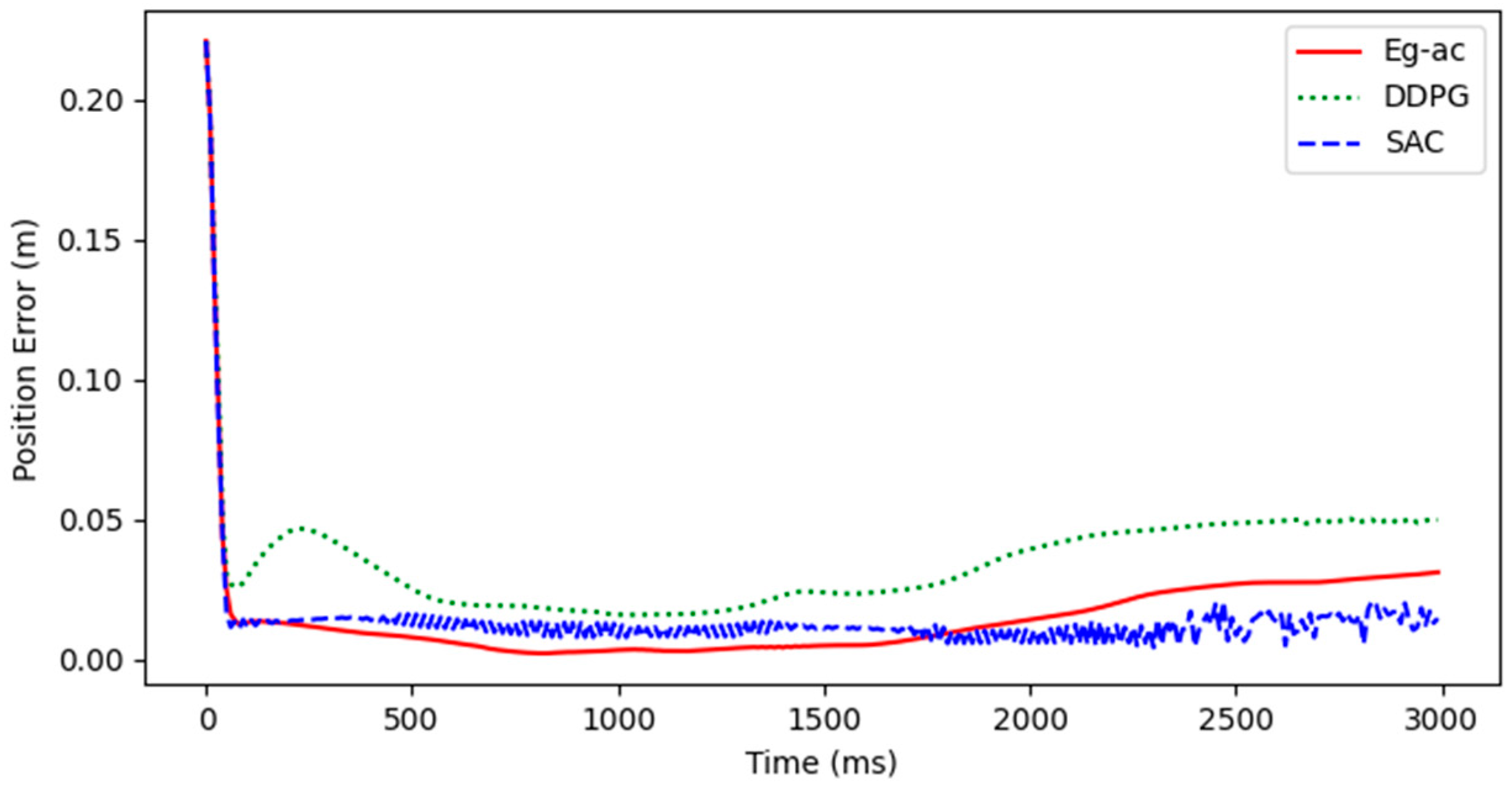
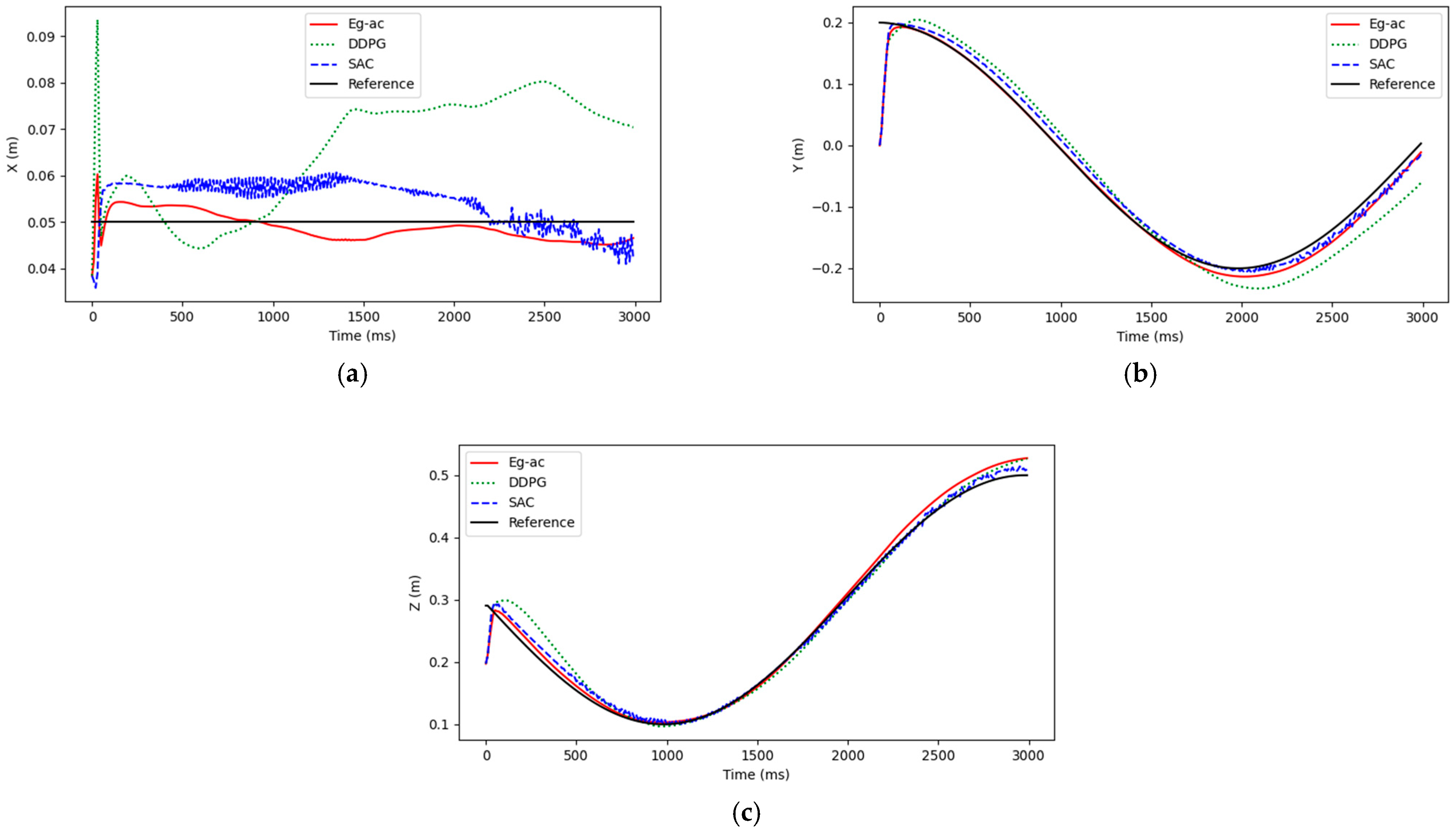
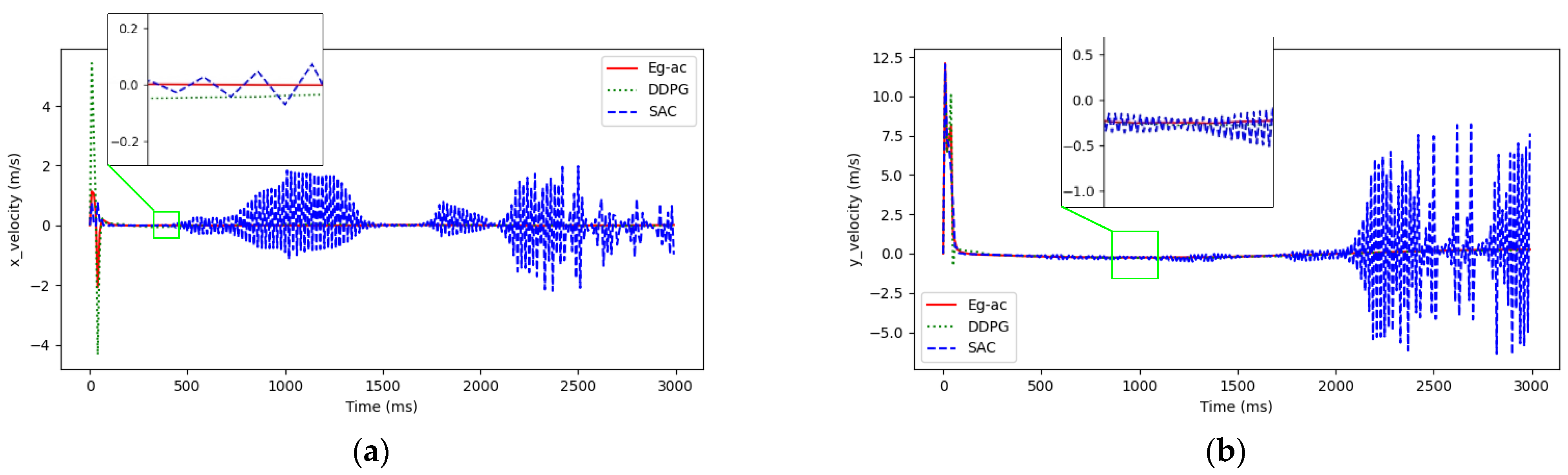
4. Simulation Results and Analysis
5. Conclusions
Supplementary Materials
Author Contributions
Funding
Data Availability Statement
Acknowledgments
Conflicts of Interest
References
- Liao, L.; Yang, Z.; Wang, C.; Xu, C.; Xu, H.; Wang, Z.; Zhang, Q. Flight Control Method of Aerial Robot for Tree Obstacle Clearing with Hanging Telescopic Cutter. Control Theory Appl. 2023, 40, 343–352. [Google Scholar]
- Wang, M.; Chen, Z.; Guo, K.; Yu, X.; Zhang, Y.; Guo, L.; Wang, W. Millimeter-Level Pick and Peg-in-Hole Task Achieved by Aerial Manipulator. IEEE Trans. Robot. 2024, 40, 1242–1260. [Google Scholar] [CrossRef]
- Kang, K.; Prasad, J.V.R.; Johnson, E. Active Control of a UAV Helicopter with a Slung Load for Precision Airborne Cargo Delivery. Unmanned Syst. 2016, 4, 213–226. [Google Scholar] [CrossRef]
- Amri bin Suhaimi, M.S.; Matsushita, K.; Kitamura, T.; Laksono, P.W.; Sasaki, M. Object Grasp Control of a 3D Robot Arm by Combining EOG Gaze Estimation and Camera-Based Object Recognition. Biomimetic 2023, 8, 208. [Google Scholar] [CrossRef]
- Villa, D.K.D.; Brandão, A.S.; Sarcinelli-Filho, M. A Survey on Load Transportation Using Multirotor UAVs. J. Intell. Robot. Syst. 2020, 98, 267–296. [Google Scholar] [CrossRef]
- Tagliabue, A.; Kamel, M.; Verling, S.; Siegwart, R.; Nieto, J. Collaborative transportation using MAVs via passive force control. In Proceedings of the IEEE International Conference on Robotics and Automation, Singapore, 29 May–3 June 2017. [Google Scholar]
- Darivianakis, G.; Alexis, K.; Burri, M.; Siegwart, R. Hybrid Predictive Control for Aerial Robotic Physical Interaction towards Inspection Operations. In Proceedings of the IEEE International Conference on Robotics & Automation, Hong Kong, China, 31 May–7 June 2014. [Google Scholar]
- Molina, J.; Hirai, S. Aerial pruning mechanism, initial real environment test. Robot. Biomim. 2018, 7, 127–132. [Google Scholar]
- Roderick, W.R.T.; Cutkosky, M.R.; Lentink, D. Bird-inspired dynamic grasping and perching in arboreal environments. Sci. Robot. 2021, 6, eabj7562. [Google Scholar] [CrossRef] [PubMed]
- Sun, X. Application of Intelligent Operation and Maintenance Technology in Power System. Integr. Circuit Appl. 2023, 40, 398–399. [Google Scholar]
- Zhang, Q.; Liao, L.; Xiao, S.; Yang, Z.; Chen, K.; Wang, Z.; Xu, H. Research on the aerial robot flight control technology for transmission line obstacle clearance. Appl. Sci. Technol. 2023, 50, 57–63. [Google Scholar]
- Suarez, A.; Heredia, G.; Ollero, A. Physical-Virtual impedance control in ultralightweight and compliant Dual-Arm aerial manipulators. IEEE Robot. Autom. Lett. 2018, 3, 2553–2560. [Google Scholar] [CrossRef]
- Zhang, G.; He, Y.; Dai, B.; Gu, F.; Yang, L.; Han, J.; Liu, G. Aerial Grasping of an Object in the Strong Wind: Robust Control of an Aerial Manipulator. Appl. Sci. 2019, 9, 2230. [Google Scholar] [CrossRef]
- Nguyen, H.; Lee, D. Hybrid force/motion control and internal dynamics of quadrotors for tool operation. In Proceedings of the 2013 IEEE/RSJ International Conference on Intelligent Robots and Systems, Tokyo, Japan, 3–7 November 2013. [Google Scholar]
- Zhong, H.; Miao, Z.; Wang, Y.; Mao, J.; Li, L.; Zhang, H.; Chen, Y.; Fierro, R. A Practical Visual Servo Control for Aerial Manipulation Using a Spherical Projection Model. IEEE Trans. Ind. Electron. 2020, 67, 10564–10574. [Google Scholar] [CrossRef]
- Alexis, K.; Huerzeler, C.; Siegwart, R. Hybrid predictive control of a coaxial aerial robot for physical interaction through contact. Control Eng. Pract. 2014, 32, 96–112. [Google Scholar] [CrossRef]
- Zhuo, H.; Yang, Z.; You, Y.; Xu, N.; Liao, L.; Wu, J.; He, J. A Hierarchical Control Method for Trajectory Tracking of Aerial Manipulators Arms. Actuators 2024, 13, 333. [Google Scholar] [CrossRef]
- Mnih, V.; Kavukcuoglu, K.; Silver, D.; Rusu, A.A.; Veness, J.; Bellemare, M.G.; Graves, A.; Riedmiller, M.; Fidjeland, A.K.; Ostrovski, G.; et al. Human-level control through deep reinforcement learning. Nature 2015, 518, 529. [Google Scholar] [CrossRef] [PubMed]
- Hasselt, H.V.; Guez, A.; Silver, D. Deep reinforcement learning with double q-learning. arXiv 2015, arXiv:1509.06461. [Google Scholar] [CrossRef]
- Qiu, Z.; Liu, Y.; Zhang, X. Reinforcement Learning Vibration Control and Trajectory Planning Optimization of Translational Flexible Hinged Plate System. Eng. Appl. Artif. Intell. 2024, 133, 108630. [Google Scholar] [CrossRef]
- Yang, A.; Chen, Y.; Naeem, W.; Fei, M.; Chen, L. Humanoid motion planning of robotic arm based on human arm action feature and reinforcement learning. Mechatronics 2024, 7, 102630. [Google Scholar] [CrossRef]
- Zhang, S.; Xia, Q.; Chen, M.; Cheng, S. Multi-Objective Optimal Trajectory Planning for Robotic Arms Using Deep Reinforcement Learning. Sensors 2023, 23, 5974. [Google Scholar] [CrossRef]
- Mnih, V.; Kavukcuoglu, K.; Silver, D.; Graves, A.; Antonoglou, I.; Wierstra, D.; Riedmiller, M. Playing Atari with Deep Reinforcement Learning. arXiv 2013, arXiv:1312.5602. [Google Scholar]
- Peters, J.; Schaal, S. Policy Gradient Methods for Robotics. In Proceedings of the 2006 IEEE/RSJ International Conference on Intelligent Robots and Systems, Beijing, China, 9–15 October 2006; pp. 2219–2225. [Google Scholar]
- Silver, D.; Lever, G.; Heess, N.; Degris, T.; Wierstra, D.; Riedmiller, M. Deterministic Policy Gradient Algorithms. In Proceedings of the 31st International Conference on Machine Learning (ICML-14), Beijing, China, 21–26 June 2014; pp. 387–395. [Google Scholar]
- Haarnoja, T.; Zhou, A.; Hartikainen, K.; Tucker, G.; Ha, S.; Tan, J.; Kumar, V.; Zhu, H.; Gupta, A.; Abbeel, P.; et al. Soft Actor-Critic Algorithms and Applications. arXiv 2019, arXiv:1812.05905. [Google Scholar]
- Lillicrap, T.P.; Hunt, J.J.; Pritzel, A.; Heess, N.; Erez, T.; Tassa, Y.; Silver, D.; Wierstra, D. Continuous control with deep reinforcement learning. arXiv 2015, arXiv:1509.02971. [Google Scholar]
- Fujimoto, S.; van Hoof, H.; Meger, D. Addressing Function Approximation Error in Actor-Critic Methods. arXiv 2018, arXiv:1802.09477. [Google Scholar]
- Sekkat, H.; Tigani, S.; Saadane, R.; Chehri, A. Vision-based robotic arm control algorithm using deep reinforcement learning for autonomous objects grasping. Appl. Sci. 2021, 11, 7917. [Google Scholar] [CrossRef]
- Lindner, T.; Milecki, A.; Wyrwał, D. Positioning of the Robotic Arm Using Different Reinforcement Learning Algorithms. Int. J. Control. Autom. Syst. 2021, 19, 1661–1676. [Google Scholar] [CrossRef]
- Oikonomou, K.M.; Kansizoglou, I.; Gasteratos, A. A Hybrid Reinforcement Learning Approach with a Spiking Actor Network for Efficient Robotic Arm Target Reaching. IEEE Robot. Autom. Lett. 2023, 8, 3007–3014. [Google Scholar] [CrossRef]
- Song, B.Y.; Wang, G.L. A Trajectory Planning Method for Capture Operation of Space Robotic Arm Based on Deep Reinforcement Learning. J. Comput. Inf. Sci. Eng. 2024, 24, 091003-1. [Google Scholar] [CrossRef]
- Wu, P.; Su, H.; Dong, H.; Liu, T.; Li, M.; Chen, Z. An obstacle avoidance method for robotic arm based on reinforcement learning. Ind. Robot 2024, 52, 9–17. [Google Scholar] [CrossRef]
- Wu, J.; Yang, Z.; Liao, L.; He, N.; Wang, Z.; Wang, C. A State-Compensated Deep Deterministic Policy Gradient Algorithm for UAV Trajectory Tracking. Machines 2022, 10, 496. [Google Scholar] [CrossRef]
- Denavit, J.; Hartenberg, R.S. A kinematic notation for lower-pair mechanisms based on matrices. Trans. ASME J. Appl. Mech. 1955, 22, 215–221. [Google Scholar] [CrossRef]
- Hinton, G.E.; Srivastava, N.; Krizhevsky, A.; Sutskever, I.; Salakhutdinov, R.R. Improving neural networks by preventing coadaptation of feature detectors. Comput. Sci. 2012, 3, 212–223. [Google Scholar]

| Symbol | Explanation |
|---|---|
| 1 | 0 | 0 | 0 | |
| 2 | −90° | 0 | 0 | |
| 3 | 0 | 0 | ||
| 4 | 0 | 0 | ||
| 5 | 90° | 0 | 0 |
Disclaimer/Publisher’s Note: The statements, opinions and data contained in all publications are solely those of the individual author(s) and contributor(s) and not of MDPI and/or the editor(s). MDPI and/or the editor(s) disclaim responsibility for any injury to people or property resulting from any ideas, methods, instructions or products referred to in the content. |
© 2025 by the authors. Licensee MDPI, Basel, Switzerland. This article is an open access article distributed under the terms and conditions of the Creative Commons Attribution (CC BY) license (https://creativecommons.org/licenses/by/4.0/).
Share and Cite
Wu, J.; Yang, Z.; Zhuo, H.; Xu, C.; Liao, L.; Cheng, D.; Wang, Z. Encouraging Guidance: Floating Target Tracking Technology for Airborne Robotic Arm Based on Reinforcement Learning. Actuators 2025, 14, 66. https://doi.org/10.3390/act14020066
Wu J, Yang Z, Zhuo H, Xu C, Liao L, Cheng D, Wang Z. Encouraging Guidance: Floating Target Tracking Technology for Airborne Robotic Arm Based on Reinforcement Learning. Actuators. 2025; 14(2):66. https://doi.org/10.3390/act14020066
Chicago/Turabian StyleWu, Jiying, Zhong Yang, Haoze Zhuo, Changliang Xu, Luwei Liao, Danguo Cheng, and Zhiyong Wang. 2025. "Encouraging Guidance: Floating Target Tracking Technology for Airborne Robotic Arm Based on Reinforcement Learning" Actuators 14, no. 2: 66. https://doi.org/10.3390/act14020066
APA StyleWu, J., Yang, Z., Zhuo, H., Xu, C., Liao, L., Cheng, D., & Wang, Z. (2025). Encouraging Guidance: Floating Target Tracking Technology for Airborne Robotic Arm Based on Reinforcement Learning. Actuators, 14(2), 66. https://doi.org/10.3390/act14020066