A Symmetrical RRPRR Robust Coupling for Crossed Axes Transmission

Abstract

A new coupling solution for transmitting the rotation motion between two shafts with crossed axes is proposed. Based on structural considerations, a planar (P) pair is introduced into the structure of the mechanism, presenting the advantage of reduced costs due to the constructive and manufacturing simplicity and to high reliability. The proposed mechanism is of the RRPRR type, and the structural symmetry simplifies substantially the construction of the mechanism. The constructive parameters of the mechanism are the angle and distance between the driving and driven shaft and also the length of the common normal between the axes of driving and driven revolute (R) pairs, and the axes of the revolute pairs of the coupling chain, respectively. Due to the presence of the planar pair, the Hartenberg–Denavit method of homogenous operators is not applicable. The kinematic analysis for a specified motion of the driving element requires two stages: finding the relative motions from the revolute pairs and the motions from the planar pair. The RRPRR transmission is analysed for geometrical asymmetrical and symmetrical cases; the latter is more convenient and the design principles are presented. Concerning the dimensional optimization, it is found to be a methodology for ensuring that the transmission ratio of the mechanism can be maintained within a stipulated range. Based on the kinematical calculus and geometrical optimization, the mechanism was designed and manufactured.

1. Introduction

In engineering systems the issue of ensuring a certain motion for a specific element of a mechanical structure often arises. The problem is solved using a kinematical chain that ensures the transmission of motion from the driving element (the actuator) to the final element (the effector). The classical approach of the problem assumes the use of a typical actuator with simple motion, and then, the kinematic chain has the role of transforming the simple motion from the actuator to a complex motion required by the final element. Another manner of solving the problem consists in using a signal generator capable of ensuring the desired motion to the effector which is rigidly coupled to the actuator.

Referring to the first solution, the most difficult task is to stipulate the structure and the dimensions of the coupling kinematic chain [1,2]. A first imposed requirement of structural order, is to ensure to the transmission mechanism a degree of freedom equal to the number of the driving elements. In practical engineering, there are quite rare cases when a mechanism is capable of ensuring to the final element a law of motion identical to the expected one [3].

In most situations, the obtained law of motion approximates the theoretical one with a certain error. The dimensional optimization of the mechanisms should be based on the next optimization criterion: the deviation between the actual and theoretical law of motion should be kept between pre-set limits. Unlike the dimensional optimization which is a continuous process, as Hunt [4] mentions, the structural optimization is iterative. Thus, if a dimensional solution that ensures the optimization criteria cannot be found for an adopted structure, then, this structural solution must be aborted and a new one must be searched for.

The main objective of our work is to provide a new constructive solution, simple and robust, for coupling two shafts with crossed axes (non-co-planar) whose axes are not obliged to maintain a fixed position (the relative position of the axes may modify in time).The mechanisms with planar pairs are less used in practice [5], mainly due to the high number of degrees of freedom (three) which must be controlled. But the application of planar pairs in the structure of a mechanism presents the advantage of the reduced costs of these pairs, due to the constructive and manufacturing simplicity and to high reliability given by the contact on large regions between the surfaces of the contacting elements [6]. To identify a possible structural solution containing planar pairs, one should start from the mobility of a spatial mechanism, found with the following relation:

$$M_f=(6-f)(n-1)-{\sum }_{k=f+1}^5(k-f)c_k$$

(1)

where $M_f$ is the mobility, defined as the number of scalar independent parameters required to describe univocally the position of the mechanism; $f$ is the family of the mechanism, defined as the number of common constraints imposed on all mobile elements of the mechanisms; $n$ is the number of elements of the mechanism; $c_k$ is the number of pairs of class $k$; the class of a kinematic pair is defined as the number of cancelled degrees of freedom for one element of the pair when the other element is considered immobile; the class can take values between 1 and 5.

The employment of Equation (1) allows for finding the structure of a mechanism when certain (different) structural conditions are imposed. As an example, let us consider that a structural solution that permits the transmission of motion between two shafts with crossed axes by direct contact, as in Figure 1, is sought.

To apply the Equation (1), it is accepted a priori that the situation of the most general case of spatial mechanism (as a consequence, $f=0$) exists [7], that is, the mobility of the mechanisms should be $M_0=1$, meaning that a single driving element exists. The mechanism has $(0,1,2)=3$ elements: the mobile elements 1 and 2 are linked to the ground by revolute pairs A and B, of the fifth class and between these two elements is formed a pair of class $C_x$ that supresses x degrees of freedom of the mechanism [8]. Equation (1) becomes:

$$1=6(n-1)-2\cdot 5-1\cdot x$$

(2)

From here:

$$1=6(3-1)-10-x$$

(3)

Equation (3) has a unique solution:

$$x=1.$$

(4)

Equation (4) shows that the single possible structural solution for transmission of motion between two shafts with crossed axes is represented by the construction of a pairs of class 1 between the two shafts. As examples of such mechanisms one may remind: of the spatial cam mechanisms [9], and the gear mechanisms with crossed axes, either with helical gears or with hypoid gears [10,11].

The challenge of introducing into the structure of the mechanism another pair, and not the class 1 pair, conducts to values of the mobility $M\le 0$, and thus the mechanism is blocked. As a consequence, the transmission of motion between the two kinematic elements cannot be obtained via a planar pair.

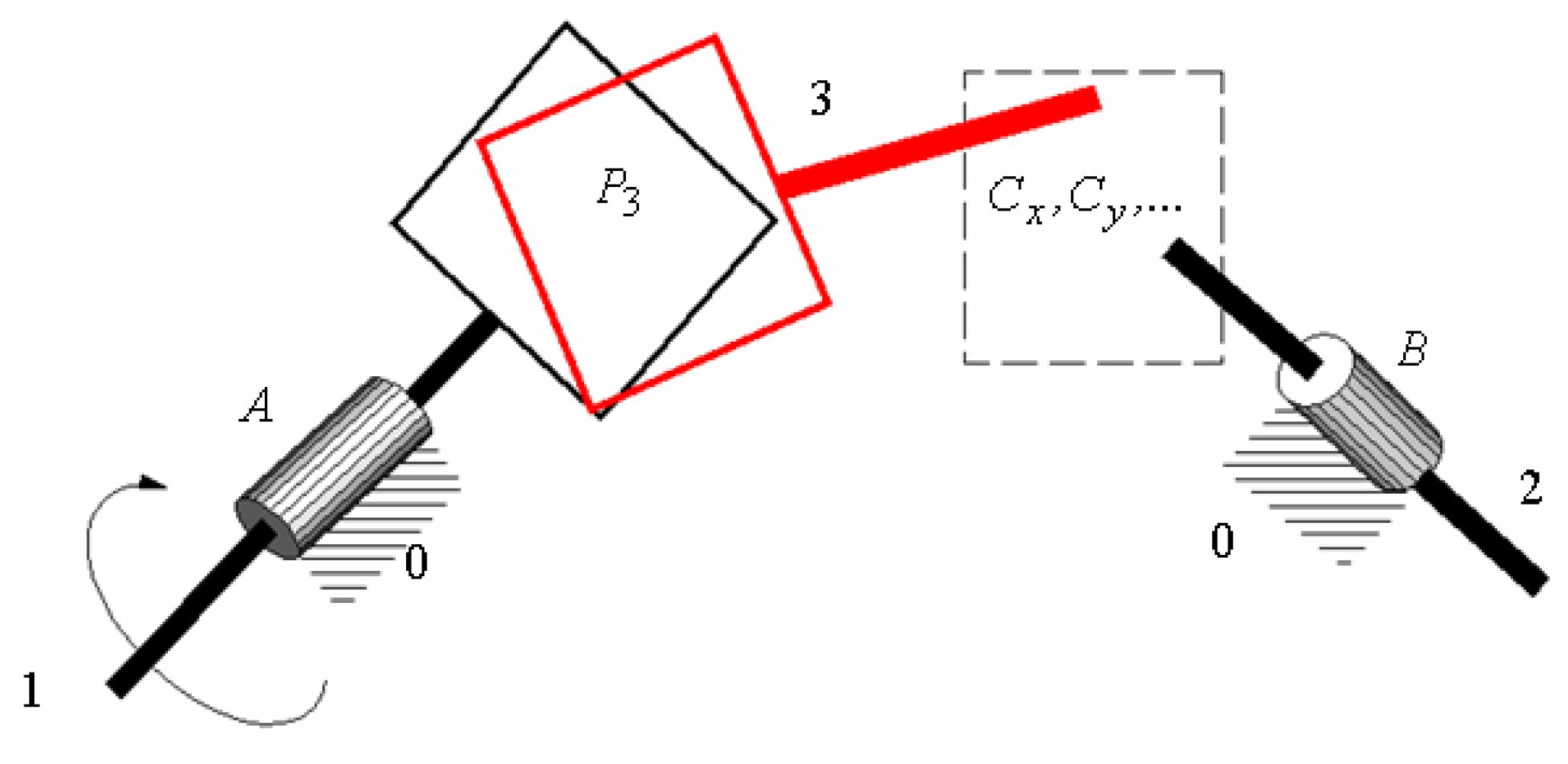
A structural solution is aimed at, to transmit the motion between the two shafts using intermediate element 3; see Figure 2.

To be remarked that for parallelism between driving and driven axes, the coupling can be substituted by a Schmidt coupling [12], or for concurrent axes, the coupling can be replaced by a Cardan joint [13], or conical gear mechanisms. The present coupling is superior to the ones mentioned from the point of view of the transmission ratio since, unlike the Cardan joint which has a variable transmission ratio, it is a homokinetic one, as will be shown. A mechanical transmission which allows for transmission of rotation motion with a constant ratio between concurrent axes is the Rzeppa joint [14]. As can be noticed, in order to replace the sliding friction with the rolling friction, the spherical bodies are moving in toroidal channels made on the surfaces of the two shafts, a fact that results in unusual manufacturing difficulties. Concerning the helical gear mechanisms (and also the Rzeppa joints), they have the kinematic advantage with respect to the proposed solution of a rigorously constant transmission ratio, but present as a disadvantage the necessity of ensuring a very well controlled relative position of the axes, and that the axes should be fixed. Additionally, the contact between the teeth of gear mechanisms is of the Hertz type, characterised by important contact surface stresses while for the proposed solution, all contacts are of the surface type (conformal), with the possibility of adopting from the design phase the dimensions of the contact regions in order to limit the values of contact pressures.

Equation (1) takes the form $M_0=1$, $n(0,1,2,3)=4$, the pairs A and B remain of the fifth class and a planar pair of class 3 ($P_3$) is formed between the elements 1 and 2, and thus, the intermediate element 3 will form other pairs of class $x$, $y$...., with the rest of the elements; see Figure 2. Here, the intuitive notation P for the planar pair was used, though other notations exist in the literature [15]; and to avoid confusions, recent works do not practice such literal symbolization [16].

In this case, Equation (1) becomes

$$1=6\left(4-1\right)-2\cdot 5-3-\left(x+y+\dots \right),$$

(5)

and conducts to:

$$x+y+\dots =4.$$

(6)

Equation (6) shows that the rest of the pairs possibly formed by the intermediate element can be of class maximum 4, and there are several possible structural solutions. When a minimum number of pairs is desired, the single probable structural solution is $x=4$, $y=x=\dots =0$ and corresponds to the case when the intermediate element forms with the other mobile element a class four cylindrical pair [17]. The obtained mechanism, RPCR, presented in Figure 3 is detailed constructively and kinematical analysed in [18]. The demand of obtaining a mechanism with symmetrical structure of the $RP{C}_{x}PR$ type result in the following particular form of Equation (1):

$$1=6(4-1)-2\cdot 5-2\cdot 3-x$$

(7)

that has the solution x = 1; see example in Figure 4. Therefore, if the mechanism contains two revolute pairs and two planar pairs, the existence of an additional class 1 pairs is necessary for obtaining a well determined motion. The condition of having structural symmetry of the mechanism is related to the idea that the single viable solution is that this class 1 pair should be formed either between the driven and driving element, or between the intermediate element and the ground.

The constructive solution of the last variant is presented in [19]. As can be observed from Figure 5, the application of the class 1 pair is not simple; the constructive solution of transmission becomes complex and, furthermore, the concentrated contact will induce significant contact stresses.

So, the conclusion of avoiding higher pairs in the structure of the kinematic chain emerges and leads to the idea of using as coupling solution a kinematic chain formed by two elements, 2 and 4, that form between them a planar pair of class $C_3$ and also, form a mechanism with symmetric structure. The structural symmetry condition is related to the requirement that the elements of the intermediate coupling chain form with each of the driving and driven elements a pair of the same class $c_x$. For this case, in Equation (1), $n\left(0,1,2,3,4\right)=5$ elements; two revolute pairs of class 5, A and B; a planar pair $P_3$ of class 3; two pairs $C_x$ of the same class x as in Figure 6.

The mobility of the mechanism remains the same:

$$1=6(5-1)-2\cdot 5-2\cdot 3-2x$$

(8)

From here,

$$x=5.$$

(9)

In conclusion, the unknown pairs have to be of class 5 (revolute, translation or helical). From these three variants, the revolute pair was the option since it can be materialized by rolling bearings. Additionally, one can remark that for the crossed axes, both the double Cardan joint and the present mechanism, the sliding friction was not avoided, in the prismatic pair and in the planar pair, respectively. Another solution that can be applied for the transmission of rotation motion with a constant ratio, between crossed axes, is represented by the mechanism with tripodic [20] or bipodic contact. This results, with the exception of the planar pair, in all other pairs of the mechanism, the rolling friction is ensured, a fact that provides higher efficiency [21]. It must be mentioned that the correct running of the mechanism requires that the revolution axes Δ^′ and Δ^″ of the new formed revolute pairs not be parallel to $\mathit{n}$, the normal to the contact plane of the planar pair; see Figure 7. If this condition is not obeyed, an uncontrolled revolute motion could appear in the intermediate revolute pair which links the element of the planar pair to the input element and to the output element, respectively.

2. Materials and Method

2.1. Method of Homogenous Operators;Principle of the Method

The kinematic analysis of spatial mechanisms can be made following the method developed by Hartenberg and Denavit [22,23] based on matrix calculus. The method is suitable to all mechanisms that have on their structure only revolute pairs, with the particular aspects of revolution, translation or helical motion. The mechanisms that obey this condition, that is, contain pairs for which an axis of relative motion can be identified, are named H-D mechanisms, while the ones which do not satisfy this condition (since they contain pairs for which we cannot stipulate an axis of relative motion between the elements of the pair) are called non H-D mechanisms. The Hartenberg–Denavit method is founded on the transformation relation for the coordinates of a point when the reference frame is changed. Two Cartesian reference systems $\left(p\right)$ and $\left(q\right)$ are considered, as in Figure 8. A point $M$ has the coordinates $M(x_p,y_p,z_p)$ in $\left(p\right)$ system and $M(x_q,y_q,z_p)$ in $\left(q\right)$ system. It is aimed at obtaining the calculus relations of the coordinates in the $\left(p\right)$ frame when the coordinates are known and the position of the system (the origin $O_q$ and the orientation of the versors ${\mathit{i}}_q,{\mathit{j}}_q,{\mathit{k}}_q$), in the $\left(q\right)$ frame, as in Figure 8.

The relation between the position vectors of the point $M$ in the two coordinate systems is:

$${\mathit{r}}_M^{\left(p\right)}={\mathit{r}}_{O_q}^{\left(p\right)}+{\mathit{r}}_M^{\left(q\right)}$$

(10)

where ${\mathit{r}}_M^{\left(p\right)}$, ${\mathit{r}}_M^{\left(q\right)}$ are the position vectors of point $M$ in the two frames (the exponent represents the coordinate system in which the vector is stipulated) and ${\mathit{r}}_{Oq}^{\left(p\right)}$ is the position vector of the origin of system $\left(q\right)$ in system $\left(p\right)$. Expressing the vectors from relation (10) using the versors of the coordinate axes, results in

$$x_p{\mathit{i}}_p+y_p{\mathit{j}}_p+z_p{\mathit{k}}_p=x_{O_q}^{\left(p\right)}{\mathit{i}}_p+y_{O_q}^{\left(p\right)}{\mathit{j}}_p+z_{O_q}^{\left(p\right)}{\mathit{k}}_p+x_q{\mathit{i}}_q+y_q{\mathit{j}}_q+z_q{\mathit{k}}_q\left|·{\mathit{i}}_p,{\mathit{j}}_p,{\mathit{k}}_p\right.$$

(11)

The above relation is projected on the axes of system $\left(p\right)$ and conducts to three scalar equations which can be expressed in matrix format, as follows:

$$\left[\begin{array}{c}{x}_p\\ y_p\\ z_p\end{array}\right]=\left[\begin{array}{c}{x}_{O_q}^{\left(p\right)}\\ y_{O_q}^{\left(p\right)}\\ z_{O_q}^{\left(p\right)}\end{array}\right]+\left[\begin{array}{ccc}{i}_q\cdot i_p& j_q\cdot i_p& k_q\cdot i_p\\ i_q\cdot j_p& j_q\cdot j_p& k_q\cdot j_p\\ i_q\cdot k_p& j_q\cdot k_p& k_q\cdot k_p\end{array}\right]\cdot \left[\begin{array}{c}{x}_q\\ y_q\\ z_q\end{array}\right]$$

(12)

Equation (12) can be written in a concentrated manner, as proposed by McCarthy [24,25]:

$${\mathit{x}}_p={\mathit{d}}_{pq}+{\mathit{R}}_{pq}{\mathit{x}}_q$$

(13)

where the components of the displacement that superposes system $\left(p\right)$ over system $\left(q\right)$ are:

$${\mathit{d}}_{pq}=\left[\begin{array}{c}{x}_{O_q}^{\left(p\right)}\\ y_{O_q}^{\left(p\right)}\\ z_{O_q}^{\left(p\right)}\end{array}\right], R_{pq}=\left[\begin{array}{ccc}{i}_q\cdot i_p& j_q\cdot i_p& k_q\cdot i_p\\ i_q\cdot j_p& j_q\cdot j_p& k_q\cdot j_p\\ i_q\cdot k_p& j_q\cdot k_p& k_q\cdot k_p\end{array}\right]$$

(14)

The vector corresponding to the translation of point $O_p$ in $O_q$ is ${\mathit{d}}_{pq}$ and ${\mathit{R}}_{pq}$ is the matrix corresponding to the rotation that superposes the axes of frame ($p$) over the axes of frame ($q$). When three systems ($p$), ($q$), ($r$) are considered, the displacement of the initial system ($p$) over the final system ($r$) is straightforward, with the matrix relation as follows:

$${\mathit{x}}_p={\mathit{d}}_{pr}+{\mathit{R}}_{pr}{\mathit{x}}_r$$

(15)

or by passing through the intermediate system $\left(q\right)$:

$${\mathit{x}}_p={\mathit{d}}_{pq}+{\mathit{R}}_{pq}{\mathit{x}}_q={\mathit{d}}_{pq}+{\mathit{R}}_{pq}({\mathit{d}}_{qr}+{\mathit{R}}_{qr}{\mathit{x}}_r)=({\mathit{d}}_{pq}+{\mathit{R}}_{pq}{\mathit{d}}_{qr})+{\mathit{R}}_{pq}{\mathit{R}}_{qr}{\mathit{x}}_r$$

(16)

The displacement and rotations from relations (15) and (16) are identified, resulting in

$$\left\{\begin{array}{c}{d}_{pr}=\left(d_{pq}+R_{pq}{d}_{qr}\right)\\ R_{pr}=R_{pq}{R}_{qr}\end{array}\right.$$

(17)

Relations (17) show that the final rotation matrix can be obtained by the simple matrix product between the rotation matrices in the order of their effectuation but the displacement vector does not result by a simple addition of the vectors corresponding to translations. The relation will be more complex with the increase in the number of intermediate frames used for attending the final system. To overpass this drawback, Hartenberg and Denavit considered that the tri-dimensional motion from the space ($x,y,z$) is a glide in the hyperplane ($w=1$) tetra-dimensional Cartesian space ($x,y,z,w$). This motion is described by the following matrix equation:

$$\left[\begin{array}{c}\underset{\left(3x1\right)}{x_p}\\ 1\end{array}\right]=\left[\begin{array}{cc}\underset{\left(3x3\right)}{R_{pq}}& \underset{\left(3x1\right)}{d_{pq}}\\ \begin{array}{ccc}0& 0& 0\end{array}& 1\end{array}\right]\left[\begin{array}{c}\underset{\left(3x1\right)}{x_p}\\ 1\end{array}\right]$$

(18)

Or, concentrated:

$${\mathit{X}}_p={\mathit{T}}_{pq}{\mathit{X}}_q$$

(19)

where:

$$\underset{\left(4x1\right)}{X_p}=\left[\begin{array}{c}{x}_p\\ 1\end{array}\right],\underset{\left(4x4\right)}{T_{pq}}=\left[\begin{array}{cc}{R}_{pq}& d_{pq}\\ \begin{array}{ccc}(0& 0& 0)\end{array}& 1\end{array}\right]$$

(20)

In the above relations $T_{pq}$ represents the displacement which superposes frame (p) over frame (q), having as components the translation of vector $d_{pq}$ and the rotation of matrix $R_{pq}$.

$$X_p=T_{pq}{X}_q=T_{pq}\left(T_{qr}{X}_r\right)=\left(T_{pq}{T}_{qr}\right)X_r$$

(21)

From Equation (21), the relation describing the composition of the matrices is:

$$T_{pr}=T_{pq}{T}_{qr}$$

(22)

From relation (22) it can be noticed that the matrix of a global displacement is obtained as a product of matrices for all successive intermediate displacements, written in the order of occurrence. Relation (22) shows the homogenous character of the coordinate transformation relations (20). For this reason, the method proposed by Hartenberg and Denavit is also called the “method of homogenous operators” [22,23]. Applying relation (22) for the displacement from frame (1) into frame (n) using the intermediate frames $\left(2\right),\left(3\right),\dots ,\left(n-1\right)$, the next relation is obtained as follows:

$$T_{1n}=T_{12}{T}_{23}\dots T_{n-1,n}$$

(23)

Now, by identifying system $(n+1)$ with system (1),

$$n+1\equiv 1$$

(24)

the following equation is obtained:

$$T_{12}{T}_{23}\dots T_{n-1.n}{T}_{n,1}=T_{\mathrm{1,1}}=I_4$$

(25)

The above equation represents the closure matrix equation for a kinematical spatial chain. This equation is similar to the vector closure equation for a plane kinematical chain and permits finding the position parameters of the kinematical chain.

Equation (23) or (25) provides 12 scalar equations. Three of these correspond to the equalities between the displacement vectors and nine equations correspond to the equality of the rotation matrices from both members of equations. From the last nine, only three equations are independent, and, to be emphasised, identifying these three independent equations is a difficult task [26]. In conclusion, either Equations (23) or (25) will result in six scalar equations that permit finding the position of the kinematic chain. The form of the scalar equations is intricate, since there are trigonometrical systems with multiple solutions corresponding to all assembling possibilities. Hartenberg and Denavit showed that for the case of a mechanism having in its structure only revolute pairs (H-D mechanism), by convenient choice of coordinate axes, the number of scalar parameters required to stipulate the relative position between two coordinate systems is reduced from six to four. For this purpose, the axes of the pairs will be the “z” axes of the coordinate systems, indexed in the order of their connection in the structure of the mechanism, while the axes “x” will be the common normals of two consecutive “z” axes. The procedure is illustrated in Figure 9.

Thus, system “k” can be superposed over system “k + 1” by performing two successive displacements: the first is a roto-translation about the “$z_k$” axis of parameters ${\theta }_k$ and $s_k$, and the second is a roto-translation about the “$x+1$” axis of parameters ${\alpha }_{k,k+1}$ and $a_{k,k+1}$.

The matrix that describes displacement of the coordinate system “k” over system “k + 1” is the following product:

$$T_{k,k+1}=Z\left({\theta }_k,s_k\right)X\left({\alpha }_{k,k+1},a_{k,k+1}\right)$$

(26)

where the matrices $Z\left({\theta }_k,s_k\right)$ and $X\left({\alpha }_{k,k+1},a_{k,k+1}\right)$, according to [25] are given by the following relation:

$$Z(\theta ,s)=\left[\begin{array}{cccc}\cos \theta & -\sin \theta & 0& 0\\ \sin \theta & \cos \theta & 0& 0\\ 0& 0& 1& s\\ 0& 0& 0& 1\end{array}\right]$$

(27)

and:

$$X(\alpha ,a)=\left[\begin{array}{cccc}1& 0& 0& a\\ 0& \cos \alpha & -\sin \alpha & 0\\ 0& \sin \alpha & \cos \alpha & 0\\ 0& 0& 0& 1\end{array}\right]$$

(28)

The matrices $\mathit{Z}(\theta ,s)$ and $\mathit{X}(\alpha ,a)$ have the property that their inverse is obtained by a plain change in the signum of arguments:

$$X(\alpha ,a{)}^{-1}=X\left(-\alpha ,-a\right)$$

(29)

$$Z(\theta ,s{)}^{-1}=Z\left(-\theta ,-s\right)$$

(30)

Relations (29) and (30) permit the calculus of the inverse of the ${\mathit{T}}_{k,k+1}$ matrix from relation (26) as follows:

$${\mathit{T}}_{k,k+1}^{-1}={\left[\mathit{Z}({\theta }_k,s_k)\mathit{X}({\alpha }_{k,k+1},a_{k,k+1})\right]}^{-1}=\mathit{X}(-{\alpha }_{k,k+1},-a_{k,k+1})\mathit{Z}(-{\theta }_k,-s_k)$$

(31)

The scalar equations obtained based on relation (25) are intricate trigonometric equations. To simplify the results, McCarthy proposes the re-writing of Equation (25) under the following form:

$$T_{12}{T}_{23}\dots T_{k-1,k}=(T_{k,k+1}\dots T_{n-1.n}{T}_{n,1}{)}^{-1}$$

(32)

McCarthy recommends that the ground of the mechanism should be the separation element and the index $\mathrm{“}k\mathrm{”}$ should be chosen in a manner that both terms of Equation (32) contains, if possible, the same number of unknowns.

For the H-D mechanisms, Uicker [27] proposes a numerical algorithm for solving Equation (25), an algorithm which considers all 12 scalar equations obtained from matrix Equation (25).

2.2. Obtaining the Motions from the Revolute Pairs

The Hartenberg-Denavit method is applicable only for the mechanisms formed by kinematical chains having in the structure only revolute pairs, (having the axis of motion well stipulated, H-D linkages) with the following particular cases: revolute pair, translational pair or helical pair. If other types of pairs occur in the structure of the mechanism, (non H-D kinematical chains), the method is not applicable. A solution for overpassing this drawback consists in structural equivalation of all non H-D pairs with revolute pairs, and afterwards, the H-D method can be applied. This manner has the disadvantage that complex kinematical chains result in very difficult calculus [28].

In actual applications, given the non H-D pairs have more degrees of freedom, the geometrical creating conditions are simpler. For example, in the case of a lower non H-D pair of class three: the geometric conditions impose that three non-coplanar points from an element should appertain to a plane attached to the other element, and for the spherical pair, it is sufficient that a point from one of the elements coincides to another point (attached to) from the other element. The difficulty of imposing such conditions consists in the fact that they impose relations between geometrical elements placed on different elements. In order to express the conditions of creating a pair in mathematical form, it is required that all the parameters characteristic of the geometries of the two elements of the pair are expressed in the same reference system. This can be made simple, by applying the transformation relations presented above, namely the method of homogenous operators proposed by Hartenberg and Denavit.

In Figure 10 is presented the scheme of the symmetric non H-D mechanism RRPRR. The mechanism contains the driving element 1 and driven element 2, each linked to the ground by a revolute pair. Between the two elements, the motion is transmitted via a non H-D kinematic chain, consisting in the intermediate elements 3 and 4, between which a planar pair is formed. Elements 3 and 4 of the intermediate kinematic chain are linked to elements 1 and 2 by revolute pairs, respectively. The axes of the intermediate revolute pairs are normal to the axes of the pairs linked to the ground.

The axes of the revolute pairs were denoted according the Hartenberg-Denavit methodology, with $z_k,k=1,2,3,4$. The geometrical creating cnditions for the planar pair between elements 3 and 4 will be expressed in a reference frame attached to the ground. The coordinate system $“0”$ fixed to the ground has the $O{x}_0$ axis along the common normal of the axes $z_1$ and $z_2$, (input and output axes), and the origin $O$ is placed at the middle of the minimum distance between them. $O{z}_0$ is placed in the bisecting plane of the dihedral angle formed by the plane defined by the axes $O{x}_0$ and $z_1$, and $O{x}_0$ and $z_2$, respectively. The $O{y}_0$ axis completes a right Cartesian reference system.

As mentioned, in order to make the planar pair, it is required that the planes $\left(P_3\right)$ and $\left(P_4\right)$ should be in coincidence, in any moment, as in Figure 11. This necessity is fulfilled if three noncolinear points from one of the planes also belong to the other plane.

The vector form for expressing the condition that the points $A_k,k=\mathrm{1,2},3$ from plane 4$P\left(4\right)$ belong to $\left(P_3\right)$ is:

$$\mathit{n}\cdot \overline{O_3{A}_k}=0,k=\mathrm{1,2},3$$

(33)

where $O_3$ is the origin of reference system 3, as in Figure 10. Relations (33) offer three scalar equations on unknowns, the angles ${\theta }_2$, ${\theta }_3$, and ${\theta }_4$ from the rotation pairs of the mechanism. The vectors and the points from relations (33) have well-stipulated components, both in frame 3 (${\mathit{n}}_3$ and $O_3$), and in frame 4, the points $A_k,k=1,2,3$. In order to operate with relations (33), all the vectors and all the coordinates of the points must be expressed in the same coordinate system. According to McCarthy [25], it is recommended that the coordinate system should be structural, equally distanced from systems 3 and 4; thus, a frame attached to the ground $x_0,y_0,z_0$ was chosen, of origin and orientation presented in Figure 10.

The displacement that takes system 0 over system 3 has the homogenous operator ${\mathit{T}}_{03}$:

$$\begin{array}{c}{T}_{03}=X\left({\displaystyle \frac{\pi }{2}}-\alpha ,-a\right)Z({\theta }_1,s_1)X\left(-{\displaystyle \frac{\pi }{2}},0\right)Z\left({\theta }_3,0\right)=\\ =\left[\begin{array}{cccc}\mathrm{c}\mathrm{o}\mathrm{s}{\theta }_1\mathrm{c}\mathrm{o}\mathrm{s}{\theta }_3& -\mathrm{c}\mathrm{o}\mathrm{s}{\theta }_1\mathrm{s}\mathrm{i}\mathrm{n}{\theta }_3& -\mathrm{s}\mathrm{i}\mathrm{n}{\theta }_1& -a\\ \mathrm{s}\mathrm{i}\mathrm{n}\alpha \mathrm{s}\mathrm{i}\mathrm{n}{\theta }_1\mathrm{c}\mathrm{o}\mathrm{s}{\theta }_3+\mathrm{c}\mathrm{o}\mathrm{s}\alpha \mathrm{s}\mathrm{i}\mathrm{n}{\theta }_3& -\mathrm{s}\mathrm{i}\mathrm{n}\alpha \hspace{0.17em}\mathrm{s}\mathrm{i}\mathrm{n}{\theta }_1\mathrm{s}\mathrm{i}\mathrm{n}{\theta }_3+\mathrm{c}\mathrm{o}\mathrm{s}\alpha \mathrm{c}\mathrm{o}\mathrm{s}{\theta }_3& \mathrm{s}\mathrm{i}\mathrm{n}\alpha \hspace{0.17em}\mathrm{c}\mathrm{o}\mathrm{s}{\theta }_1& -\mathrm{c}\mathrm{o}\mathrm{s}\alpha \hspace{0.17em}{s}_1\\ \mathrm{c}\mathrm{o}\mathrm{s}\alpha \mathrm{s}\mathrm{i}\mathrm{n}{\theta }_1\mathrm{c}\mathrm{o}\mathrm{s}{\theta }_3-\mathrm{s}\mathrm{i}\mathrm{n}\alpha \mathrm{s}\mathrm{i}\mathrm{n}{\theta }_3& -\mathrm{c}\mathrm{o}\mathrm{s}\alpha \mathrm{s}\mathrm{i}\mathrm{n}{\theta }_1\mathrm{s}\mathrm{i}\mathrm{n}{\theta }_3-\mathrm{s}\mathrm{i}\mathrm{n}\alpha \mathrm{c}\mathrm{o}\mathrm{s}{\theta }_3& \mathrm{c}\mathrm{o}\mathrm{s}\alpha \mathrm{c}\mathrm{o}\mathrm{s}{\theta }_1& \mathrm{s}\mathrm{i}\mathrm{n}\alpha \hspace{0.17em}{s}_1\\ 0& 0& 0& 1\end{array}\right]\end{array}$$

(34)

In a similar manner, the displacement of ground 0 over frame 4 has the matrix ${\mathit{T}}_{04}$:

$$\begin{array}{c}{T}_{04}=X\left(-{\displaystyle \frac{\pi }{2}}+\alpha ,a\right)Z({\theta }_2,s_2)X\left({\displaystyle \frac{\pi }{2}},0\right)Z({\theta }_4,0)=\\ =\left[\begin{array}{cccc}\mathrm{c}\mathrm{o}\mathrm{s}{\theta }_2\mathrm{c}\mathrm{o}\mathrm{s}{\theta }_4& -\mathrm{c}\mathrm{o}\mathrm{s}{\theta }_2\mathrm{s}\mathrm{i}\mathrm{n}{\theta }_4& \mathrm{s}\mathrm{i}\mathrm{n}{\theta }_2& a\\ \mathrm{s}\mathrm{i}\mathrm{n}\alpha \mathrm{s}\mathrm{i}\mathrm{n}{\theta }_2\mathrm{c}\mathrm{o}\mathrm{s}{\theta }_4+\mathrm{c}\mathrm{o}\mathrm{s}\alpha \mathrm{s}\mathrm{i}\mathrm{n}{\theta }_4& -\mathrm{s}\mathrm{i}\mathrm{n}\alpha \mathrm{s}\mathrm{i}\mathrm{n}{\theta }_2\mathrm{s}\mathrm{i}\mathrm{n}{\theta }_4+\mathrm{c}\mathrm{o}\mathrm{s}\alpha \mathrm{c}\mathrm{o}\mathrm{s}{\theta }_4& -\mathrm{s}\mathrm{i}\mathrm{n}\alpha \mathrm{c}\mathrm{o}\mathrm{s}{\theta }_2& s_2\mathrm{c}\mathrm{o}\mathrm{s}\alpha \\ -\mathrm{c}\mathrm{o}\mathrm{s}\alpha \mathrm{s}\mathrm{i}\mathrm{n}{\theta }_2\mathrm{c}\mathrm{o}\mathrm{s}{\theta }_4+\mathrm{s}\mathrm{i}\mathrm{n}\alpha \mathrm{s}\mathrm{i}\mathrm{n}{\theta }_4& \mathrm{c}\mathrm{o}\mathrm{s}\alpha \mathrm{s}\mathrm{i}\mathrm{n}{\theta }_2\mathrm{s}\mathrm{i}\mathrm{n}{\theta }_4+\mathrm{s}\mathrm{i}\mathrm{n}\alpha \mathrm{c}\mathrm{o}\mathrm{s}{\theta }_4& \mathrm{c}\mathrm{o}\mathrm{s}\alpha \mathrm{c}\mathrm{o}\mathrm{s}{\theta }_2& s_2\mathrm{s}\mathrm{i}\mathrm{n}\alpha \\ 0& 0& 0& 1\end{array}\right]\end{array}$$

(35)

In order to obtain the projection of the normal $\mathit{n}$ to the common contact plane of the planar pair, one can use the relation:

$$n=T_{03}{n}_3=T_{03}\begin{array}{cccc}[0& 1& 0& 0{]}^T\end{array}=\left[\begin{array}{c}-\cos {\theta }_1\sin {\theta }_3\\ -\sin \alpha \hspace{0.17em}\sin {\theta }_1\sin {\theta }_3+\cos \alpha \cos {\theta }_3\\ -\cos \alpha \hspace{0.17em}\hspace{0.17em}\sin {\theta }_1\sin {\theta }_3-\sin \alpha \cos {\theta }_3\\ 1\end{array}\right]$$

(36)

or the relation:

$$n=T_{04}{n}_4=T_{04}\begin{array}{cccc}[0& 1& 0& 0{]}^T\end{array}=\left[\begin{array}{c}\cos {\theta }_2\sin {\theta }_4\\ \sin \alpha \hspace{0.17em}\sin {\theta }_2\sin {\theta }_4-\cos \alpha \cos {\theta }_4\\ -\cos \alpha \hspace{0.17em}\hspace{0.17em}\sin {\theta }_2\sin {\theta }_4-\sin \alpha \cos {\theta }_4\\ 1\end{array}\right]$$

(37)

It can be remarked that relation (36) is preferable because it contains only one of the unknowns, ${\theta }_3$, while in relation (37), both ${\theta }_2$ and ${\theta }_4$ are present. The vector ${\mathit{r}}_0=\overline{O{O}_3}$ has the components in frame 0 given by

$$r_0=T_{03}{\left[\begin{array}{cccc}0& 0& 0& 1\end{array}\right]}^T=\left[\begin{array}{c}-a\\ -s_1\cos \alpha \\ s_1\sin \alpha \\ 1\end{array}\right]$$

(38)

The vectors ${\mathit{r}}_1,{\mathit{r}}_2$, and ${\mathit{r}}_3$ are the position vectors in frame $0$ for the noncolinear points $A_1$, $A_2$, and $A_3$ belonging to plane $O_4{x}_4{z}_4$ from frame 4. For the general case, relations (33) have a difficult form. To simplify this form, three particular points were selected, having in frame $4$ the coordinates: $A_1(0,0,\zeta )$, $A_2(0,0,-\zeta )$, and $A_3(\xi ,0,0)$, as in Figure 11. The position vectors of these points in frame $0$ will have the following form:

$$r_1=T_{04}\left[\begin{array}{c}0\\ 0\\ \zeta \\ 1\end{array}\right]=\left[\begin{array}{c}a+\zeta \sin {\theta }_2\\ s_2\cos \alpha -\zeta \hspace{0.17em}\sin \alpha \cos {\theta }_2\\ s_2\hspace{0.17em}\sin \hspace{0.17em}\alpha +\zeta \cos \alpha \cos {\theta }_2\hspace{0.17em}\\ 1\end{array}\right]$$

(39)

$$r_2=T_{04}\left[\begin{array}{c}0\\ 0\\ -\zeta \\ 1\end{array}\right]=\left[\begin{array}{c}a+\zeta \sin {\theta }_2\\ s_2\cos \alpha +\zeta \hspace{0.17em}\sin \alpha \cos {\theta }_2\\ s_2\hspace{0.17em}\sin \hspace{0.17em}\alpha -\zeta \cos \alpha \cos {\theta }_2\hspace{0.17em}\\ 1\end{array}\right]$$

(40)

$$r_3=T_{04}\left[\begin{array}{c}\xi \\ 0\\ 0\\ 1\end{array}\right]=\left[\begin{array}{c}a+\xi \cos {\theta }_2\cos {\theta }_4\\ s_2\cos \alpha +\xi \sin \alpha \sin {\theta }_2\cos {\theta }_4+\xi \cos \alpha \hspace{0.17em}\sin {\theta }_4\\ s_2\sin \alpha -\xi \cos \alpha \hspace{0.17em}\hspace{0.17em}\sin {\theta }_2\cos {\theta }_4+\xi \sin \alpha \hspace{0.17em}\hspace{0.17em}\sin {\theta }_4\\ 1\end{array}\right]$$

(41)

By replacing Equations (36), (39), (40) and (41) in relations (33), three scalar equations result, of unknowns the angles ${\theta }_2$, ${\theta }_3$, and ${\theta }_4$ corresponding to the rotations about the axes $z_2$, $z_3$, and $z_4$, respectively. The actual form of the equations is complicated:

$$\left\{\begin{array}{c}(\cos 2\alpha +s_1/s_2)\cos {\theta }_3-\left[\right(2a/s_2)\cos {\theta }_1+\sin 2\alpha \sin {\theta }_1]\sin {\theta }_3=0\\ \cos 2\alpha \sin {\theta }_1\cos {\theta }_2+\cos {\theta }_1\sin {\theta }_2\sin {\theta }_3+\sin 2\alpha \cos {\theta }_2\cos {\theta }_3=0\\ (\cos 2\alpha \cos {\theta }_3-\sin 2\alpha \sin {\theta }_1\sin {\theta }_3)\sin {\theta }_4+\left[\right(\sin 2\alpha \cos {\theta }_3+\cos 2\alpha \sin {\theta }_1\sin {\theta }_3)\sin {\theta }_2-\cos {\theta }_1\cos {\theta }_2\sin {\theta }_3]\cos {\theta }_4+\\ +(\cos 2\alpha \sin {\theta }_1\cos {\theta }_2+\cos {\theta }_1\sin {\theta }_2\sin {\theta }_3+\sin 2\alpha \cos {\theta }_2\cos {\theta }_3)=0\end{array}\right.$$

(42)

It is remarked that, the term from Equation (42), which does not contain the unknown ${\theta }_4$, is identical to the left member of the second equation of the system and, therefore, it is zero. So, the final form of system (42) is

$$\left\{\begin{array}{c}(\mathit{cos}2\alpha +s_1/s_2){\mathit{cos\theta }}_3-\left[\right(2a/s_2){\mathit{cos\theta }}_1+\mathit{sin}2\alpha {\mathit{sin\theta }}_1]{\mathit{sin\theta }}_3=0\\ \left[\mathit{cos}2\alpha {\mathit{sin\theta }}_1+\mathit{sin}2\alpha {\mathit{cos\theta }}_3]{\mathit{cos\theta }}_2+\right({\mathit{cos\theta }}_1{\mathit{sin\theta }}_3){\mathit{sin\theta }}_2=0\\ \left[\right(\mathit{sin}2\alpha {\mathit{cos\theta }}_3+\mathit{cos}2\alpha {\mathit{sin\theta }}_1{\mathit{sin\theta }}_3){\mathit{sin\theta }}_2-{\mathit{cos\theta }}_1{\mathit{cos\theta }}_2{\mathit{sin\theta }}_3]{\mathit{cos\theta }}_4+(\mathit{cos}2\alpha {\mathit{cos\theta }}_3-\mathit{sin}2\alpha {\mathit{sin\theta }}_1{\mathit{sin\theta }}_3){\mathit{sin\theta }}_4=0\end{array}\right.$$

(43)

It can be noticed that the equations of system (43) can be written in the following form:

$$A_k{\mathit{cos\theta }}_k+B_k{\mathit{sin\theta }}_k=0$$

(44)

where the coefficients $A_k$ and $B_k$ are knowns, since they can be found with the values of the unknowns from the previous equations. System (43) has the following solutions:

$$\left\{\begin{array}{c}{\theta }_3=\mathit{atan}{\displaystyle \frac{\mathit{cos}2\alpha +s_1/s_2}{\left(\frac{2a}{s_2}\right){\mathit{cos\theta }}_1+\mathit{sin}2\alpha {sin\theta }_1}}+k_1\pi ,k_1\in \mathit{Z}\\ {\theta }_2=-\mathit{atan}{\displaystyle \frac{\mathit{cos}2\alpha {\mathit{sin\theta }}_1{\mathit{sin\theta }}_3+\mathit{sin}2\alpha { cos\theta }_3}{{\mathit{cos\theta }}_1{\mathit{sin\theta }}_3}}+k_2\pi ,k_2\in \mathit{Z}\\ {\theta }_4=-\mathit{atan}{\displaystyle \frac{(\mathit{sin}2\alpha {\mathit{cos\theta }}_3+\mathit{cos}2\alpha {\mathit{sin\theta }}_1{\mathit{sin\theta }}_3){\mathit{sin\theta }}_2-{\mathit{cos\theta }}_1{\mathit{cos\theta }}_2{\mathit{sin\theta }}_3}{\mathit{cos}2\alpha {\mathit{cos\theta }}_3-\mathit{sin}2\alpha {\mathit{sin\theta }}_1{sin\theta }_3}}+k_3\pi ,k_3\in \mathit{Z}\end{array}\right.$$

(45)

In Equation (45), $k_1,k_2,k_3$ are numbers belonging to integer numbers $\mathit{Z}$ To choose these values of $k_1$, $k_2$, $k_3$ in a manner that the theoretical model matches the actual mechanism is a difficult task. In order to unburden this selection duty, the mechanism was modelled in a simplified manner using the DMUKinematics/CATIA Dassault software module [29], as shown in Figure 12. This model results in $2a=20 \mathrm{m}\mathrm{m}$; $2\alpha =20°$; $s_1=50 \mathrm{m}\mathrm{m}$ and $s_2=80 \mathrm{m}\mathrm{m}$.

With these values, for a given position angle ${\theta }_{10}=22.11°$ of driving element 1, ${\theta }_{20}=-25.027°$,${ \theta }_{30}=77.03°$, ${\theta }_{40}=-94.901°$ were obtained, and afterwards, the variation in the three rotation angles was represented as a function of the position angle of the driving element, as in Figure 13, Figure 14 and Figure 15. The discontinuities occurring in the models of the revolutions from the pairs of the mechanism, in Figure 16, are caused by the presence of the function $\mathit{atan}(x)$ in relations (45) of the displacements, a function that has the co-domain $[-\pi /2,\pi /2]$, corresponding to a $\pi rad$ revolution.

A complete revolution requires a function of co-domain of length $2\pi$. The computing utilitaries provide inverse trigonometric functions of two arguments which satisfy this requirement (the $2\pi$ length co-domain) from which we can recall: $\mathit{atan}2(x,y)$ having the co-domain; $\left[\mathrm{0,2}\pi \right]$, $\mathit{arg}(x+iy)$ having the co-domain $[-\pi ,\pi ]$, and $angle(x,y)$ having the co-domain $\left[\mathrm{0,2}\pi \right]$ [30].

For modelling the kinematic of the mechanism in concordance with the continuity conditions imposed on the displacements of the actual mechanism, the Equation (45) were written as follows:

$$\left\{\begin{array}{c}{\theta }_3=\mathit{arg}[(2a/s_2){\mathit{cos\theta }}_1+\mathit{sin}2\alpha {\mathit{sin\theta }}_1+i(\mathit{cos}2\alpha +s_1/s_2)]\\ {\theta }_2=-angle({\mathit{cos\theta }}_1{\mathit{sin\theta }}_3,\mathit{cos}2\alpha {\mathit{sin\theta }}_1{\mathit{sin\theta }}_3+\mathit{sin}2\alpha {\mathit{cos\theta }}_3)\\ {\theta }_4=-\mathit{arg}\{\mathit{cos}2\alpha {\mathit{cos\theta }}_3-\mathit{sin}2\alpha {\mathit{sin\theta }}_1{\mathit{sin\theta }}_3+i\left[\right(\mathit{sin}2\alpha {\mathit{cos\theta }}_3+\mathit{cos}2\alpha {\mathit{sin\theta }}_1{\mathit{sin\theta }}_3){\mathit{sin\theta }}_2-{\mathit{cos\theta }}_1{\mathit{cos\theta }}_2{\mathit{sin\theta }}_3)\}-\pi \end{array}\right.$$

(46)

In Figure 17, Figure 18 and Figure 19 are represented the displacements found with relations (45) (in red line) and relations (46) (blue line), and the values obtained, for a stipulated position of the driving element, with the kinematic simulation software (circle symbols). The derivatives of the three rotations expressed by relations (46) are represented in Figure 20 and a continuity of angular velocities is remarked. Additionally, driven element 2 has a rotatory motion as the sign of the derivative of the signal is constant, while in the intermediate revolute pairs, the motions are oscillations (the angles ${\theta }_3$ and ${\theta }_4$), because the derivatives of these angles present periodical variations in sign.

2.3. Finding the Motions from the Planar Pair

The planar pair is a class 3 pair and permits $6-3=3$ degrees of freedom between its elements, that is a rotation about the normal to the common contact plane and two translations in the contact plane. In order to define the rotation, it is necessary to find the angle between two straight lines, each one attached to an element of the pair. For this case, the angle between the versors ${\mathit{k}}_4$ and ${\mathit{k}}_3$ will be determined. Considering that each of the two versors has the coordinates stipulated in different systems of reference,

$$k_4^{\left(4\right)}={\left[\begin{array}{cccc}0& 0& 1& 0\end{array}\right]}^T,{ k}_3^{\left(3\right)}={\left[\begin{array}{cccc}0& 0& 1& 0\end{array}\right]}^T$$

(47)

results in the necessity of expressing them in the same frame. Here, the most convenient is the frame of the ground. Thus,

$$k_4^{\left(0\right)}=T_{04}{k}_4^{\left(4\right)}=\left[\begin{array}{c}\sin {\theta }_2\\ -\sin \alpha \cos {\theta }_2\\ \cos \alpha \cos {\theta }_2\\ 0\end{array}\right]$$

(48)

$$k_3^{\left(0\right)}=T_{03}{k}_3^{\left(3\right)}=\left[\begin{array}{c}\sin {\theta }_1\\ -\sin \alpha \cos {\theta }_1\\ \cos \alpha \cos {\theta }_1\\ 0\end{array}\right]$$

(49)

An issue occurring when only the versors ${\mathit{k}}_4$ and ${\mathit{k}}_3$ are used is the occurrence of an ambiguity generated by the fact that there are two different positions of the versor ${\mathit{k}}_4$ relative to ${\mathit{k}}_3$ for which the dot product ${\mathit{k}}_4\cdot {\mathit{k}}_3$ has the same value. These two positions of the versor ${\mathit{k}}_4$ make the same angle with the versor ${\mathit{k}}_3$, but one is in a trigonometric and the other is in a clock-wise sense relative to ${\mathit{k}}_3$. To eliminate this ambiguity, the versor ${\mathit{i}}_3^{\left(0\right)}$ is also determined, defining the oriented angle between the versors ${\mathit{k}}_4$ and ${\mathit{k}}_3$:

$$i_3^{\left(0\right)}=T_{03}{i}_0^{\left(3\right)}=T_{03}\left[\begin{array}{c}1\\ 0\\ 0\\ 0\end{array}\right]=\left[\begin{array}{c}\cos {\theta }_1\cos {\theta }_3\\ \sin \alpha \sin {\theta }_1\cos {\theta }_3+\cos a\sin {\theta }_3\\ \cos \alpha \sin {\theta }_1\cos {\theta }_3-\sin \alpha \sin {\theta }_3\\ 0\end{array}\right]$$

(50)

The rotation angle ${\theta }_{43}$ made by the axis $z_4$ with the axis $z_3$ is

$${\theta }_{43}=angle({\mathit{k}}_4\cdot {\mathit{i}}_3,{\mathit{k}}_4\cdot {\mathit{k}}_3)-{\displaystyle \frac{\pi }{2}}$$

(51)

Or, in explicit manner,

$${\theta }_{43}=angle\left[\begin{array}{c}\mathit{cos}2\alpha {\mathit{sin\theta }}_1{\mathit{cos\theta }}_2{\mathit{cos\theta }}_3+{\mathit{cos\theta }}_1{\mathit{sin\theta }}_2{\mathit{cos\theta }}_3-\mathit{sin}2\alpha {\mathit{cos\theta }}_2{\mathit{sin\theta }}_3,\\ \mathit{cos}2\alpha {\mathit{cos\theta }}_1{\mathit{cos\theta }}_2-{\mathit{sin\theta }}_1{\mathit{sin\theta }}_2\end{array}\right]-{\displaystyle \frac{\pi }{2}}$$

(52)

The variation in the oriented angle between the axes $z_4$ and $z_3$ is represented in Figure 21a; the variation in the angular velocity from the planar joint is presented in Figure 21b and it can be noticed that the motion is oscillatory because the angular velocity changes its sign.

To characterise the relative displacements from the planar pair, two planes attached to each of the elements of the pair are considered; the trajectory of a point belonging to one plane is required, with respect to the other plane. Considering from the plane $O_3{x}_3{z}_3$, a point of coordinates:

$$r_3^{\left(3\right)}={\left[\begin{array}{cccc}{x}_3& 0& z_3& 1\end{array}\right]}^T$$

(53)

In order to find the coordinates ${\mathit{r}}_3^{\left(4\right)}$, the relation for coordinate transformation is applied:

$${\mathit{r}}_3^{\left(4\right)}={\mathit{T}}_{43}{\mathit{r}}_3^{\left(3\right)}$$

(54)

where the homogenous operator ${\mathit{T}}_{43}$, in explicit form, is:

$$\begin{array}{l}{T}_{43}=T_{40}{T}_{03}={\left(T_{04}\right)}^{-1}{T}_{03}=\\ ={\left[\mathit{X}\left(-{\displaystyle \frac{\pi }{2}}+\alpha ,a\right)\mathit{Z}({\theta }_2,s_2)\mathit{X}\left({\displaystyle \frac{\pi }{2}},0\right)\mathit{Z}({\theta }_4,0)\right]}^{-1}\mathit{X}\left({\displaystyle \frac{\pi }{2}}-\alpha ,-a\right)\mathit{Z}({\theta }_1,s_1)\mathit{X}\left(-{\displaystyle \frac{\pi }{2}},0\right)\mathit{Z}\left({\theta }_3,0\right)=\\ =\mathit{Z}(-{\theta }_4,0)\mathit{X}\left(-{\displaystyle \frac{\pi }{2}},0\right)\mathit{Z}(-{\theta }_2,-s_2)\mathit{X}\left({\displaystyle \frac{\pi }{2}}-\alpha ,-a\right)\mathit{X}\left({\displaystyle \frac{\pi }{2}}-\alpha ,-a\right)\mathit{Z}({\theta }_1,s_1)\mathit{X}\left(-{\displaystyle \frac{\pi }{2}},0\right)\mathit{Z}\left({\theta }_3,0\right)\end{array}$$

(55)

After performing the calculus, the following expression is obtained:

$$\begin{array}{l}{x}_3^{\left(4\right)}=x_3\left[\begin{array}{c}({\mathit{sin\theta }}_3{\mathit{sin\theta }}_4-{\mathit{sin\theta }}_1{\mathit{sin\theta }}_2{\mathit{cos\theta }}_3{\mathit{cos\theta }}_4)\mathit{cos}2\alpha +\\ ({\mathit{sin\theta }}_2{\mathit{sin\theta }}_3{\mathit{cos\theta }}_4+{\mathit{sin\theta }}_1{\mathit{cos\theta }}_3{\mathit{sin\theta }}_4)\mathit{sin}2\alpha +{\mathit{cos\theta }}_1{\mathit{cos\theta }}_2{\mathit{cos\theta }}_3{\mathit{cos\theta }}_4\end{array}\right]\\ +z_3\left[\mathit{sin}2\alpha {\mathit{cos\theta }}_1{\mathit{sin\theta }}_4-\mathit{cos}2\alpha {\mathit{sin\theta }}_2{\mathit{cos\theta }}_4-{\mathit{sin\theta }}_1{\mathit{cos\theta }}_2{\mathit{cos\theta }}_4\right]\\ -2a{\mathit{cos\theta }}_2{\mathit{cos\theta }}_4-s_1(\mathit{cos}2\alpha {\mathit{sin\theta }}_4+\mathit{sin}2\alpha {\mathit{sin\theta }}_2{\mathit{cos\theta }}_4)-s_2{sin\theta }_4\\ y_3^{\left(4\right)}=0\\ z_3^{\left(4\right)}=x_3\left[{\mathit{cos\theta }}_1{\mathit{sin\theta }}_2{\mathit{cos\theta }}_3+\mathit{cos}2\alpha {\mathit{sin\theta }}_1{\mathit{cos\theta }}_2{\mathit{cos\theta }}_3-\mathit{sin}2\alpha {\mathit{cos\theta }}_2{sin\theta }_3\right]\\ \hspace{1em}\hspace{1em}\hspace{1em}\hspace{1em}\hspace{1em}\hspace{1em}+z_3(\mathit{cos}2\alpha {\mathit{cos\theta }}_1{\mathit{cos\theta }}_2-{\mathit{sin\theta }}_1{\mathit{sin\theta }}_2)+s_1\mathit{sin}2\alpha {\mathit{cos\theta }}_2-2a {sin\theta }_2\end{array}$$

(56)

The comparison between analytical and numerical trajectories is intended: the point of coordinates $r_3^{\left(3\right)}=[\begin{array}{cccc}80& 0& 30& 1{]}^T\end{array}$ from the plane $O_3{x}_3{z}_3$ has the trajectory in the plane $O_4{x}_4{z}_4$ found with relation (56) as represented in Figure 22a, and the trajectory simulated using the kinematic software module is presented in Figure 22b. The coordinate grids traced on both plots allow for quantitative comparison and an excellent agreement between the two curves is remarked.

In a similar manner, the trajectory is described in the plane $O_3{x}_3{z}_3$ by a point belonging to the plane $O_4{x}_4{z}_4$. The transformation relation of the coordinates of the point

$$r_4^{\left(4\right)}={\left[\begin{array}{cccc}{x}_4& 0& z_4& 1\end{array}\right]}^T$$

(57)

from system $4$ in system $3$ is

$${\mathit{r}}_4^{\left(3\right)}={\mathit{T}}_{43}{\mathit{r}}_4^{\left(4\right)}$$

(58)

where the homogenous operator of transformation ${\mathit{T}}_{43}$ is given by the relation

$$\begin{array}{l}{T}_{43}={\mathit{T}}_{30}{\mathit{T}}_{04}=({\mathit{T}}_{03}{)}^{-1}{T}_{04}=\\ ={\left[\mathit{X}\left({\displaystyle \frac{\pi }{2}}-\alpha ,-a\right)\mathit{Z}({\theta }_1,s_1)\mathit{X}\left(-{\displaystyle \frac{\pi }{2}},0\right)\mathit{Z}\left({\theta }_3,0\right)\right]}^{-1}\mathit{X}\left(-{\displaystyle \frac{\pi }{2}}+\alpha ,a\right)\mathit{Z}({\theta }_2,s_2)\mathit{X}\left({\displaystyle \frac{\pi }{2}},0\right)\mathit{Z}({\theta }_4,0)\\ \hspace{1em}\hspace{1em}\hspace{1em}\hspace{1em}\hspace{1em}\hspace{1em}=\mathit{Z}\left(-{\theta }_3,0\right)\mathit{X}\left({\displaystyle \frac{\pi }{2}},0\right)\mathit{Z}(-{\theta }_1,-s_1)\mathit{X}\left(-{\displaystyle \frac{\pi }{2}}+\alpha ,a\right)\mathit{X}\left(-{\displaystyle \frac{\pi }{2}}+\alpha ,a\right)\mathit{Z}({\theta }_2,s_2)\mathit{X}\left({\displaystyle \frac{\pi }{2}},0\right)\mathit{Z}({\theta }_4,0)\end{array}$$

(59)

By replacing in relation (58) the expressions of ${\mathit{r}}_4^{\left(4\right)}$ and ${\mathit{T}}_{43}$, from relations (57) and (59), the next relation is obtained after a series of calculus:

$$\begin{array}{l}{x}_4^{\left(3\right)}=x_4\left[\begin{array}{c}({\mathit{sin\theta }}_1{\mathit{cos\theta }}_3{\mathit{sin\theta }}_4+{\mathit{sin\theta }}_2{\mathit{sin\theta }}_3{\mathit{cos\theta }}_4)\mathit{sin}2\alpha +\\ ({\mathit{sin\theta }}_3{\mathit{sin\theta }}_4-{\mathit{sin\theta }}_1{\mathit{sin\theta }}_2{\mathit{cos\theta }}_3{\mathit{cos\theta }}_4)\mathit{cos}2\alpha +{\mathit{cos\theta }}_1{\mathit{cos\theta }}_2{\mathit{cos}}_3{\mathit{cos\theta }}_4\end{array}\right]\\ +z_4\left(\mathit{cos}2\alpha {\mathit{sin\theta }}_1{\mathit{cos\theta }}_2{\mathit{cos\theta }}_3-\mathit{sin}2\alpha {\mathit{cos\theta }}_2{\mathit{sin\theta }}_3+{\mathit{cos\theta }}_1{\mathit{sin\theta }}_2 {\mathit{cos\theta }}_3\right)\\ +2a{\mathit{cos\theta }}_1{\mathit{cos\theta }}_3+s_1{\mathit{sin\theta }}_3+s_2(\mathit{cos}2\alpha {\mathit{cos\theta }}_3+\mathit{sin}2\alpha {\mathit{sin\theta }}_1{\mathit{cos\theta }}_3)\\ y_4^{\left(3\right)}=0\\ z_4^{\left(3\right)}=x_4(\mathit{sin}2a{\mathit{cos\theta }}_1{\mathit{sin\theta }}_4-\mathit{cos}2\alpha {\mathit{cos\theta }}_1{\mathit{sin\theta }}_2{\mathit{cos\theta }}_4-{\mathit{sin\theta }}_1{\mathit{cos\theta }}_2{\mathit{cos\theta }}_4)\\ \hspace{1em}\hspace{1em}\hspace{1em}\hspace{1em}\hspace{1em}+z_4\left(\mathit{cos}2\alpha \right){\mathit{cos\theta }}_1{\mathit{cos\theta }}_2-{\mathit{sin\theta }}_1{\mathit{sin\theta }}_2)-2a{\mathit{sin\theta }}_1+s_2\mathit{sin}2\alpha {cos\theta }_1\end{array}$$

(60)

The correctness of relations (60) is proved by the comparison presented in Figure 23, where the comparison of trajectories of the point $r_4^{\left(4\right)}={\left[\begin{array}{cccc}80& 0& 30& 1\end{array}\right]}^T$ from the plane $O_4{x}_4{z}_4$ is traced in the plane $O_3{x}_3{z}_3$. For a fixed point from system 4, the analytical trajectory was traced using relation (60) and the numerical one was traced using the simulation software, in the plane from system 3.

3. Results and Discussions

As shown in the previous paragraph, the mechanism has a symmetrical structure with respect to the ground. The constructive parameters of the mechanism are as follows: the angle $2\alpha$ between the input and output axes,$z_1$ and $z_{2 }$, respectively; the length $2a$ of the common normal of these axes and $s_1$ and $s_2$, the lengths of common normals of axes $z_0$ and $z_3$, and, $z_0$ and $z_4$ respectively.

The process of design and optimization of the mechanism involves only the parameters $s_1$ and $s_2$ because the values of the parameters $2a$ and $2\alpha$, characterizing the relative position between the in and out axes imposed by the project thematic.

The design and optimization of the mechanism should consider two aspects:

• Ensuring a transmission ratio which varies between pre-set limits;
• Design of the pair capable to ensure a minimum contact zone able to transmit the torques corresponding to adequate operating and to avoid the interference between the two elements of the planar pair.

A constructive sketch of the mechanism is presented in Figure 24. The contacting regions which form the higher pair have rectangular shape. A good transmission of the forces between the elements requires finding the traces described by the straight lines Δ₃ and Δ₄ in the common contact plane.

Assuming that the contact zones from both elements of the higher pair have rectangular shapes and equal dimensions, using the simulation software, the geometrical loci described by the two straight lines Δ₃ and Δ₄ were found, as presented in Figure 24.

The trajectories from Figure 25 were obtained for the next values of the following parameters: $2a=0 \mathrm{m}\mathrm{m}$;$2\alpha =20°$; $s_1=50 \mathrm{m}\mathrm{m}; s_2=80 \mathrm{m}\mathrm{m}; 2r=60 \mathrm{m}\mathrm{m}; x_0=80 \mathrm{m}\mathrm{m}$, where $2r$ and $x_0$ are the dimensions of the active rectangular zone. Applying relations (56) and (60), the analytical traces of the two straight lines in the common contact plane were obtained; the results are represented in Figure 26; the difference between the traces can be noticed, and for both lines, during operation, there will exist regions of the traces situated outside the rectangular zone (plotted with black line). The calculus was repeated for other parameters, $s_1=s_2=100 \mathrm{m}\mathrm{m}$ and the traces from Figure 27 were obtained, from which it is remarked that the two traces are identical in shape and position but are situated outside the rectangular region. Thus, a geometrical symmetry will be recommended, because, when suitable dimensions are ensured for one trace, the other trace will have the same dimensions. A second conclusion emerging from here is that for equal values of the parameters $s_1$ and $s_2$, there is the risk that the traces are positioned outside the zones assumed for contact.

From Figure 26 and Figure 27 show the major significance of the parameter $s=s_1=s_2$ upon the dimensions of the contact region from the planar pair.

In order to evaluate the effect of the three constructive paraments $2a,$ $2\alpha$, and $s$ upon the transmission ratio $i_{12}$ of the mechanism, an analytical expression of the ratio is necessary. According to the definition relation:

$$i_{12}={\displaystyle \frac{{\omega }_1}{{\omega }_2}}={\displaystyle \frac{\frac{d{\theta }_1}{dt}}{\frac{d{\theta }_2\left({\theta }_1\right)}{dt}}}={\displaystyle \frac{\frac{d{\theta }_1}{dt}}{\frac{d{\theta }_2\left({\theta }_1\right)}{d{\theta }_1}\frac{d{\theta }_1}{dt}}}={\displaystyle \frac{1}{\frac{d{\theta }_2\left({\theta }_1\right)}{d{\theta }_1}}}$$

(61)

Analysing relations (46) which give the displacements from the revolute pairs as functions of the angle ${\theta }_1$ of the driving element, one can remark that the angle ${\theta }_2$ depends on the angle ${\theta }_1$ both directly and via the angle ${\theta }_3\left({\theta }_1\right)$. Considering that, for the calculus of the transmission ratio $i_{12}$ it is necessary for the derivative of ${\theta }_2$ with respect to ${\theta }_1$ and the derivatives of the angles ${\theta }_2$ and ${\theta }_3$ to conduct to the same continuous functions no matter if expressed by Equations (45) or (46), relations (45) will be used for the angles ${\theta }_2$ and ${\theta }_3$ because they contain inverse trigonometric functions of a single argument.

The expression of ${\theta }_3\left({\theta }_1\right)$ can be written as

$${\theta }_3=\mathit{atan}{\displaystyle \frac{1+\mathit{cos}2\alpha }{2{\frac{a}{s}\mathit{cos\theta }}_1+\mathit{sin}2\alpha sin{\theta }_1}}$$

(62)

This expression is introduced into the second Equation (45) and after calculus, it results in the following:

$${\theta }_2=-\mathit{atan}[{\mathit{tan\theta }}_1+2{\displaystyle \frac{a}{s}}\mathit{tan}\alpha ]$$

(63)

The transmission ratio can be expressed only as a function of the angle ${\theta }_1$ by the simple relation

$$i_{12}=-{\displaystyle \frac{1+[{\mathit{tan\theta }}_1+2\frac{a}{s}\mathit{tan}\alpha {]}^2}{1+{\mathit{tan}}^2{\theta }_1}}$$

(64)

Relation (64) allows for the study of the influence of the three constructive parameters upon the transmission ratio. Analysing relation (64), the main strong points of the present coupling solution are highlighted:

• The possibility of transmission of rotation motion between two crossed shafts with variable relative position
• For the particular cases $\alpha =0$, the axes of the shafts are parallel and the transmission ratio is $i_{12}=-1$; the coupling becomes a CV (constant velocity) joint and can replace an Oldham or Schmidt joint [31].
• For the case $a=0$, the ratio is also $i_{12}=-1$ and the coupling can replace a conical gear mechanism or a Rzeppa joint.
• Comparing the constructive solution of the present coupling to the ones mentioned, we can say the following:

  –

  The present joint has fewer elements, compared to Rzeppa and Schmidt joints.

  –

  Elementary boundary surfaces (cylinder or plane), compared to the Rzeppa joint, which has spherical and toroidal surfaces or compared to conical gear, which has conical flank involute surfaces.

• Based on a simpler constructive solution, the manufacturing method is simpler, precise and economical.

The effect of parameters $s$, $a$ şi $\alpha$ is highlighted in Figure 28, Figure 29 and Figure 30. For each of these parameters, a string of values was considered, between a minimum and maximum value, and the curve representing the dependence of the transmission ratio with respect to the angle of the driving element was traced. The curve corresponding to the minimum value was traced with blue, the one for the maximum value was black, and for the intermediate values the traces were red. As expected, the effect of increasing the parameters $a$ and $\alpha$ was an enlargement of the interval of variation in the transmission ratio, a fact confirmed by the plots from Figure 28 and Figure 29.

Concerning the effect of parameter $s$ (common value of $s_1$ and $s_2$), it is remarked that for increased values of this parameter, the interval of variation in the transmission ratio narrows, as in Figure 30, and from here the conclusion is that for a range of variation in the transmission ratio, a value $s_{min}$ can be found, thus ensuring that the transmission ratio is within the imposed interval.

In order to obtain the value of $s_{min}$, the expression of the maximum and minimum values of the transmission ratio is required. To this end, the derivative of $i_{12}$ is calculated:

$${\displaystyle \frac{d{i}_{12}}{d{\theta }_1}}=-4a{\displaystyle \frac{[s\mathit{cos}\alpha \mathit{cos}2\theta -a\cdot \mathit{sin}\alpha \mathit{sin}2{\theta }_1]\mathit{sin}\alpha }{s^2{\mathit{cos}}^2\alpha }}$$

(65)

The solutions of the equation:

$${\displaystyle \frac{d{i}_{12}}{d{\theta }_1}}=0$$

(66)

are:

$${\theta }_{10_k}={\displaystyle \frac{1}{2}}\mathit{atan}\left[{\displaystyle \frac{1}{\mathit{tan}\alpha }}{\displaystyle \frac{s}{a}}\right]+k{\displaystyle \frac{\pi }{2}},k\in \mathit{Z}$$

(67)

and correspond to the positions of the driving element, ${\theta }_1$, for the extreme values of the transmission ratio. The values obtained in relation (67) are replaced in relation (64) and the two extreme values are obtained, expressed with the aid of the function:

$$f(s)=-{\displaystyle \frac{1}{{\left[\sqrt{\frac{a^2}{s^2}+\frac{1}{{\mathit{tan}}^2\alpha }}+\frac{a}{s}\right]}^2{\mathit{tan}}^2\alpha }}$$

(68)

As it follows:

$$i_{12max}\left(s\right)=f\left(s\right);\hspace{1em}{i}_{12min}\left(s\right)=1/f\left(s\right)$$

(69)

The goal is that the value of the transmission ratio is as close as possible to $-1$. Therefore, if it is obligatory for the transmission ratio to be maintained within the interval $[-1-\mathit{\Delta }{i}_{12},-1+\mathit{\Delta }{i}_{12}]$, where the deviation $\mathit{\Delta }{i}_{12}$ is imposed, the transcendent equation must be solved:

$$f\left(s^{\prime }\right)=-1+\mathit{\Delta }{i}_{12};\hspace{1em}\hspace{1em}\hspace{1em}f\left(s^{″}\right)=-1-\mathit{\Delta }{i}_{12}$$

(70)

Adopting for the parameter $s$ the value $s_0$, the maximum value between $s^{\prime }$ and $s^{″}$, the transmission ratio will be inside the interval $[-1-\mathit{\Delta }{i}_{12},-1+\mathit{\Delta }{i}_{12}]$. The solving of the equations (70) is represented in Figure 31 where it is remarked that for values greater than $s_0$, the extreme values are contained in above mentioned interval.

Once the minimum value $s_{min}$ of the common normal between the in/out axes and the rotation axes of intermediate pairs is found, one can proceed to adopt the final value of this parameter, and thus, the minimum contact surface between the elements of the planar pair is guaranteed, and the interference is avoided. As mentioned, the available regions for the contact between the elements of the planar pair were chosen to be rectangular and of the same dimension, $x_0$. Adopting a common value for the two parameters $s_1$ and $s_2$ confirms the reversibility of the planar pair (the relative motion of an element with respect to the other is identical, when the roles of the two elements would be reversed). To reveal the zone occupied by one of the elements of the planar pair with respect to the other one, it is considered that both contact zones are rectangular, as in Figure 32, and using the Equations (45) and (46) the traces of one rectangle versus the second rectangle were found; in Figure 33, these traces for different values of the $x_0$ parameter are presented. In Figure 33a, the risk of non-contact exists, while in Figure 33d, the interference may occur. Therefore, the domain for $x_0$ can be adopted to avoid the extreme situations mentioned.

In Figure 34 is presented the actual symmetrical RRPRR mechanisms, designed and manufactured according to the results obtained from analytical calculus and applying the geometrical optimization considerations. The prototype we fabricated confirmed the possibility of transmitting the rotation motion between two shafts with crossed axes with variable position and also, the fact that the presence of the planar pair ensures a silent operation of the transmission. The simple surfaces (plane and cylinder) that border the elements ensure good manufacturing technology and all the elements can be manufactured on universal machine tools, a fact that leads to a low transmission cost price.

The dynamic and energy aspects of the operation of the proposed transmission are goals for future work. It is obvious that the major problem consists in the study of the phenomena occurring in the planar pair, where the sliding friction must be accepted (similar to accepting sliding friction on cam mechanisms with a flat face follower or in the gear mechanisms). We believe it is important that the obtained relations allow finding the relative motions between any of the surfaces of the pairs from the structure of the mechanism, which is essential in the estimation of normal reactions and implicitly in friction forces which in the end, are decisive in the calculus of wear and efficiency.

4. Conclusions

This paper presents a new coupling solution, which contains in the structure a planar pair, for transmitting the rotation motion between two shafts with crossed axes. The presence of the planar joint is founded on structural considerations. The planar pair has a high degree of possibilities of motion and then conducts to structural solutions that have lesser elements compared to the classical solutions which contain in their structure a cylindrical, revolute of translational pairs. The first solution possible from structural considerations must have at least an intermediate element with the role of connecting the input and output shafts through at least one planar pair.

The constructive solutions presented in previous works specify difficulties of manufacturing and constructive motives. From these reasons, we aimed at a structural solution by which, the two shafts, input and output, are coupled via a kinematic linkage made between two elements, which contain a planar joint. Accepting that the planar pair should be formed between the elements of the intermediate chain, it is shown that the pairs between it and the elements linked to the ground (the driven and driving ones) can be only rotational, and thus the mechanism is a structurally symmetric of the RRPRR type. The structural symmetry simplifies substantially the construction of the mechanism. The constructive parameters of the mechanism are the angle and distance between the driving and driven shaft and also the length of the common normal between the axes of in and out pairs, and the axes of the revolute pairs of the coupling chain, respectively.

Due to the presence of the planar pair, the mechanisms cannot be placed in the category of Hartenberg–Denavit mechanisms, for which the motion from any pair has a well-stipulated axis, and thus, the method of homogenous operators is not applicable.

The kinematic analysis of the mechanism for a specified motion of the driving element supposes the completion of two steps: finding the relative motions from the revolute pairs and then, finding the motions from the planar pair.

In order to determine the motions from revolute pairs, the geometrical conditions of planar pair creation were expressed in vector form in the coordinate frame of the ground. Homogenous operators were used for expressing all the elements occurring in the equations of constraint of the planar pair. Three scalar equations were obtained which allowed for finding the motions from the revolute pairs as a function of the motion of the driving element. The motion from the exit pair is a rotatory motion, while in the inner revolute pairs, the motions are oscillations.

For finding the motions from the planar pair, the revolute motion was first determined, and it was also of the oscillatory type; and after that, the motion from the contact plane, for a point belonging to an element of the planar pair with respect to the other element was found. It was observed that by interchanging the elements of the planar pair, a different motion was obtained. By equalising the values of the constructive parameters corresponding to the positions of the inner revolute pairs with respect to the in and out positions, it is remarked that the two motions from the planar pair became identical and the pair had a reversible character. In this particular situation, the relations characteristic to the motions from kinematical pairs were substantially reduced.

From a technical point of view, an extremely important problem is the adoption of the dimensions of the elements of the planar pair. Assuming a symmetrical geometric mechanism, it is shown with that the selection of the distance between the axes of outer and inner pairs with values greater than a minimum value, the transmission ratio of the mechanism can be maintained within a pre-defined variation interval.

Supposing that the possible contact surfaces from the planar pair are two identical rectangles, the geometrical locus described by one of these rectangles with respect to the other, was found. The result allows for adopting the constrictive parameter such as to avoid the interference between the elements of the planar pair, on one side, and to ensure a minimum contact region capable of adequately transmitting the forces from the elements of the pair, on the other side.

As a final conclusion, this paper presents anew constructive solution, simple and robust for the transmission of motion between two shafts with crossed axes. For future work, concerning the pairs of the mechanism, the problem of optimization from a tribological point of view is envisaged—the employment of rolling bearings for revolute pairs and the use of a pair of materials with antifriction properties for the elements of the planar pair, with the target of a higher transmission efficiency.

References

1. Muñoz, K.; Porez, M.; Wenger, P. Kinematic and Static Analyses of a 3-DOF Spatial Tensegrity Mechanism. In Proceedings of the Advances in Robot Kinematics, Ljubljana, Slovenia, 30 June–4 July 2024; pp. 314–323. [Google Scholar] [CrossRef]
2. Kong, X. Variable degree-of-freedom spatial mechanisms composed of four circular translation joints. J. Mech. Robot. 2021, 13, 3. [Google Scholar] [CrossRef]
3. Freudenstein, F. Design of Four-Link Mechanisms. Ph.D. Thesis, Columbia University, New York, NY, USA, 1954. Available online: https://www.proquest.com/openview/1413762cc4e6e241d2aee028d407d312/1?pq-origsite=gscholar&cbl=18750&diss=y (accessed on 1 December 2024).
4. Hunt, K.H. Kinematic Geometry of Mechanisms; Oxford University Press: Oxford, UK, 1990; pp. 30–51. [Google Scholar]
5. Uicker, J.J., Jr.; Pennock, G.R.; Shigley, J.E. Theory of Machines and Mechanisms, 4th ed.; Oxford University Press: New York, NY, USA, 2010; pp. 368–370. [Google Scholar]
6. Johnson, K.L. Contact Mechanics; Cambridge University Press: Cambridge, UK, 1985; pp. 84–106. [Google Scholar]
7. Zhao, J.; Feng, Z.; Chu, F.; Ma, N. 4-Free Motion of the End Effector of a Robot Mechanism. In Advanced Theory of Constraint and Motion Analysis for Robot Mechanisms; Elsevier: Amsterdam, The Netherlands; Academic Press: Waltham, MA, USA, 2014; pp. 113–157. [Google Scholar]
8. Zhou, T.; Huang, C.; Miao, Z.; Li, Y. Intrinsically Multi-Stable Spatial Linkages. Adv. Sci. 2024, 11, 2402127. [Google Scholar] [CrossRef]
9. Rothbart, H.A. Cam Design Handbook, 1st ed.; McGraw Hill: New York, NY, USA, 2003. [Google Scholar]
10. Litvin, F.L.; Fuentes, A. Gear Geometry and Applied Theory; Cambridge University Press: Cambridge, UK, 2004; pp. 441–474. [Google Scholar]
11. Jelaska, D.T. Gears and Gear Drives; John Wiley& Sons Ltd.: West Sussex, UK, 2012. [Google Scholar]
12. Available online: https://www.industrialmagza.com/pdf/zero-max/SCHMIDT-MGZ.pdf (accessed on 15 January 2025).
13. Wei, F.; Luo, K.; Zhang, Y.; Jiang, J. Structural Design and Kinematic Analysis of Cable-Driven Soft Robot. Actuators 2024, 13, 497. [Google Scholar] [CrossRef]
14. Pennestri, E.; Rossi, V.; Salvini, P.; Valentini, P.P.; Pulvirenti, F. Review and kinematics of Rzeppa-type homokinetic joints with straight crossed tracks. Mech. Mach. Theory 2015, 90, 142–161. [Google Scholar] [CrossRef]
15. Wang, X.; Baron, L. Topology and Geometry of Serial and Parallel Manipulators. In Parallel Manipulators, New Developments; Chapter, 8; Ryu, J.-H., Ed.; I-Tech Education and Publishing: Vienna, Austria, 2008. [Google Scholar] [CrossRef]
16. Meijaard, J.P. Modelling of kinematic higher pairs by lower pairs. Mech. Mach. Theory 2024, 191, 105515. [Google Scholar] [CrossRef]
17. Cruz, J.L.R.; Rabiela, H.J.; Segura, P.G.; González, B.V.; Acosta, A.G.B. Design of a Spatial Mechanism with Revolute-Spherical-Cylindrical-Revolute (RSCR) Kinematic Joints. JMEST 2022, 9, 15365–15368. [Google Scholar]
18. Alaci, S.; Ciornei, F.-C.; Romanu, I.-C.; Ciocirlan, T.-M.; Ciornei, M.-C. Solution for the Kinematics of Non-H-D Couplings Applied to RPCR Mechanism. Axioms 2023, 12, 357. [Google Scholar] [CrossRef]
19. Alaci, S.; Doroftei, I.; Ciornei, F.-C.; Romanu, I.-C.; Doroftei, I.-A.; Ciornei, M.-C. A New RP1PR Type Coupling for Shafts with Crossed Axes. Mathematics 2023, 11, 2025. [Google Scholar] [CrossRef]
20. Urbinati, F.; Pennestri, E. Kinematic and Dynamic Analyses of the Tripode Joint. Multibody Syst. Dyn. 1998, 2, 355–367. [Google Scholar] [CrossRef]
21. Stolarski, T.A.; Tobe, S.S. Rolling Contacts (Tribology in Practice Series), 1st ed.; John Wiley & Sons, Inc.: Hoboken, NJ, USA, 2001. [Google Scholar]
22. Hartenberg, R.; Denavit, J. Kinematic Synthesis of Linkages, 1st ed.; McGraw-Hill Inc.: New York, NY, USA, 1964; pp. 343–368. [Google Scholar]
23. Denavit, J.; Hartenberg, R.S. A kinematic notation for lower-pair mechanisms based on matrices. J. Appl. Mech. 1955, 22, 215–221. [Google Scholar] [CrossRef]
24. McCarthy, J.M.; Soh, G.S. Geometric Design of Linkages; Springer: Berlin/Heidelberg, Germany, 2010; pp. 253–279. [Google Scholar]
25. McCarthy, J.M. Introduction in Theoretical Kinematics, 3rd ed.; MIT Press: Cambridge, MA, USA, 2018; pp. 103–108. [Google Scholar]
26. Fischer, I. Dual-Number Methods in Kinematics, Statics and Dynamics; CRC Press: New York, NY, USA, 1999; pp. 54–95. [Google Scholar]
27. Uicker, J.J., Jr.; Denavit, J.; Hartenberg, R.S. An Iterative Method for the Displacement Analysis of Spatial Mechanisms. J. Appl. Mech. 1964, 31, 309–314. [Google Scholar] [CrossRef]
28. Sandor, G.N.; Kohli, D.; Hernandez, M., Jr.; Ghosal, A. Kinematic analysis of three-link spatial mechanisms containing sphere-plane and sphere-groove pairs. Mech. Mach. Theory 1984, 19, 129–138. [Google Scholar] [CrossRef]
29. Zamani, N. Mechanism Design Essentials in 3dexperience Using CATIA Application; Chapter 2; SDC Publications: Mission KS, USA, 2017; pp. 1–32. Available online: https://static.sdcpublications.com/pdfsample/978-1-63057-104-7-2.pdf (accessed on 15 November 2024).
30. Maxfield, B. Engineering with Mathcad; Butterworth-Heinemann: Oxford, UK; Elsevier: Oxford, UK, 2006; pp. 287–289. [Google Scholar]
31. Seherr-Thoss, H.C.; Schmelz, F.; Aucktor, E. Universal Joints and Driveshafts. Analysis, Design, Applications, 2nd ed.; Springer: Berlin/Heidelberg, Germany, 2006; pp. 53–79, 109–245. [Google Scholar]
Figure 1. Transmission of motion between two shafts with crossed axes.
Actuators 14 00064 g001
Figure 2. Mechanism with planar pair and intermediate coupling element (traced in red).
Actuators 14 00064 g002
Figure 3. Constructive solutions for the RPCR mechanism.
Actuators 14 00064 g003
Figure 4. Mechanism with two planar pairs and symmetric structure, RP1PR; the intermediate element is in red.
Actuators 14 00064 g004
Figure 5. Constructive solutions for the RP1PR mechanism.
Actuators 14 00064 g005
Figure 6. Spatial mechanism with symmetrical structure containing a planar pair.
Actuators 14 00064 g006
Figure 7. Mechanism with symmetrical structure with planar pair, RRPRR.
Actuators 14 00064 g007
Figure 8. The position of a point M in two coordinate reference systems, the initial in blue and the current in red.
Actuators 14 00064 g008
Figure 9. The Hartenberg-Denavit parameters.
Actuators 14 00064 g009
Figure 10. The constructive schematics of the structurally symmetrical mechanisms RRPRR: driving element 1 in magenta, driven element 2 in green and intermediate elements, 3 in red and 4 in blue.
Actuators 14 00064 g010
Figure 11. The planes that create the planar pair and the non-coplanar points chosen for the definition of the pair: in red, the plane ( P 3 ) and the system 3; in blue, the plane ( P 4 ) and the system 4.
Actuators 14 00064 g011
Figure 12. Kinematic model of the transmission obtained with CATIA module DMUKinematics. The contact zone from planar pair is purple and the elements of the pair are blue and red.
Actuators 14 00064 g012
Figure 13. The rotation angle obtained in the driven pair R2.
Actuators 14 00064 g013
Figure 14. The rotation angle from the first inner revolute pair R3.
Actuators 14 00064 g014
Figure 15. The rotation angle from the second inner revolute pair R4.
Actuators 14 00064 g015
Figure 16. The derivative of the rotation angle from the second inner revolute pair R4 presents discontinuities, which does not correspond to physical realities.
Actuators 14 00064 g016
Figure 17. The rotation angle in R2 obtained using inverse trigonometric functions of one argument (red line) and of two arguments (blue line).
Actuators 14 00064 g017
Figure 18. The rotation angle in R3 obtained using inverse trigonometric functions of one argument (red plot) and of two arguments (blue plot).
Actuators 14 00064 g018
Figure 19. The rotation angle in R4 obtained using inverse trigonometric functions of one argument (red plot) and of two arguments (blue plot).
Actuators 14 00064 g019
Figure 20. The derivative of the rotation angles, from revolute pairs R2 (red plot), R3 (blue plot), and R4 (magenta plot), obtained using inverse trigonometric functions of two arguments.
Actuators 14 00064 g020
Figure 21. The variation in the (a) rotation angle; (b) angular velocity, from the planar pair.
Actuators 14 00064 g021
Figure 22. Comparison between the trajectories described in the plane O 4 x 4 z 4 by a point from the plane O 3 x 3 z 3 belonging to the element 3: (a) analytical; (b) numerical.
Actuators 14 00064 g022
Figure 23. Comparison between the trajectories described in the plane O 3 x 3 z 3 by a point from the plane O 4 x 4 z 4 : (a) analytical; (b) numerical (the brown region belongs to element 3).
Actuators 14 00064 g023
Figure 24. Constructive draft of the mechanism.
Actuators 14 00064 g024
Figure 25. The trajectories described by the points from the most advanced segment of an element of the planar pair, in the contact plane from the other element of the pair. (the element 3 in red and the element 4 in blue and the corresponding relative trajectories).
Actuators 14 00064 g025
Figure 26. Comparison between the geometrical loci of the segments Δ3 (red) and Δ4 (blue), for the parameters 2 α = 20 ° ; 2 a = 20   m m ; s 1 = 50   m m ; s 2 = 80   m m ; x 0 = 80   m m ; r = 30   m m .
Actuators 14 00064 g026
Figure 27. Superposition of the traces of the straight lines Δ3 (red) and Δ4 (blue), for s = s 1 = s 2 = 100   m m , 2 α = 20 ° , 2 a = 20   m m , x 0 = 80   m m , r = 30   m m .
Actuators 14 00064 g027
Figure 28. The effect of the angle 2 α between the in and out axes upon the transmission ratio i 12 . The white arrow shows the incressing angle 2 α .
Actuators 14 00064 g028
Figure 29. The effect of the distance 2 a between the in and out axes upon the transmission ratio i 12 . The white arrow shows increasing distance 2 a .
Actuators 14 00064 g029
Figure 30. The effect of the distance s between the in and out axes and the intermediate revolution axes upon the transmission ratio i 12 (blue plot for s m i n and black plot for s m a x ).
Actuators 14 00064 g030
Figure 31. The dependency of extreme values of the transmission ratio on the s parameter and finding the minimum value s 0 from the condition of imposed variation limits (maximum value in red, minimum value in blue).
Actuators 14 00064 g031
Figure 32. The two rectangular regions of possible contact, magenta for element 3 and black for element 4.
Actuators 14 00064 g032
Figure 33. Traces obtained for one rectangle (in black) versus the second rectangle (in magenta): (a) x 0 = 110   m m ; ( b )   x 0 = 130   m m ; ( c )   x 0 = 160   m m ; (d) x 0 = 190   m m . Red traces are described by points belonging to lateral edges and the blue traces are described by the front egde.
Actuators 14 00064 g033
Figure 34. The actual symmetrical RRPRR mechanisms designed and executed applying these results from the paper.
Actuators 14 00064 g034
Disclaimer/Publisher’s Note: The statements, opinions and data contained in all publications are solely those of the individual author(s) and contributor(s) and not of MDPI and/or the editor(s). MDPI and/or the editor(s) disclaim responsibility for any injury to people or property resulting from any ideas, methods, instructions or products referred to in the content.