1. Introduction
Many of the commonly used pieces of equipment, such as tower cranes and gantry cranes, in production and construction are affected by factors such as air turbulence and wind, which can bring challenges to control systems; so, disturbance control becomes an urgent problem to be solved. The type of equipment is underactuated systems. In this paper, the almost disturbance decoupling (ADD) method is used to design a nonlinear controller to solve the disturbance attenuation problem. The disturbance term is handled by Young’s inequality and backstepping is used to design an ADD controller for underactuated systems. The stability of the closed-loop control system is theoretically proven based on the Lyapunov stability theory.
The ADD problem was originally proposed by [
1] for linear systems. The problem of ADD for linear systems is revisited by placing the maximum number of poles in the closed-loop solution [
2]. Linearization methods are applied to address ADD control problems for nonlinear systems. In [
3], stochastic equivalent linearization methods are used to deal with nonlinear hysteresis dynamics, but such methods may not adequately capture the dynamic properties of complex nonlinear systems. In [
4], a piezoelectric dual-chip nonlinear actuator is first linearized using a stochastic equivalent linearization method and a robust controller is designed for solving a standard ADD problem. In [
5], the linear ADD design method is applied to investigate a satellite attitude control problem by using an input/output feedback linearization method. For single-input single-output (SISO) nonlinear systems, the
gain ADD problem is established and a parameterized state feedback controller is constructed such that the
gain from the disturbance to the output is arbitrarily small by increasing its gain [
6]. The problem of ADD for SISO nonlinear systems is also investigated by using the singular perturbation method and high-gain feedback in [
7]. A new set of ADD results is obtained for SISO nonlinear systems with unstable zero dynamics [
8]. Ref. [
9] designs an ADD strategy to suppress the external position disturbance and attenuate oscillations caused by discontinuous mechanical gaps for an electrohydraulic load simulator with mechanical backlash. In [
10], for lateral motion of electric vehicles with uncertain disturbances, ADD sampled state feedback is developed to attenuate the effect of the disturbance on the output with arbitrary accuracy. The adaptive stabilization control problem of uncertain high-order fully actuated (HOFA) nonlinear systems with disturbances is studied, an ADD method is employed to handle unknown disturbances, and a novel adaptive ADD controller is proposed in [
11]. In [
12], an HOFA design method is proposed to control HOFA systems with disturbances, and a weak disturbance decoupling controller is designed for HOFA nonlinear systems to ensure the stability of the closed-loop system and the desired output tracking performance while mitigating the effects of disturbances. The study in [
13] proposes a nonsingular terminal sliding mode active disturbance rejection decoupling controller for a three-dimensional autonomous underwater vehicle to achieve efficient trajectory tracking and enhance the disturbance rejection capability. In [
14], for nonlinear systems with normal form, a fixed-time ADD controller is constructed to attenuate the impact of disturbances on the states of the closed-loop system. For nonlinear systems with unknown disturbances, by using the backstepping design technique, an ADD state feedback controller is designed to ensure the internal stability of the closed-loop system and boundness of the
gain from disturbance to output [
15]. In [
16,
17], the concept of fuzzy approximate disturbance decoupling is introduced for multiple-input multiple-output (MIMO) uncertain nonlinear systems, and a fuzzy adaptive ADD controller is proposed. It is worth noting that the publications mentioned above address the ADD control problem for actuated systems. ADD control for underactuated systems has not been investigated so far.
Commonly used nonlinear control methods for real systems include backstepping, block backstepping, predictive control, fuzzy logic, neural networks, sliding mode control, output tracking, adaptive control, and so on. In this paper, the backstepping method is primarily employed to handle the impact of disturbances for uncertain underactuated nonlinear systems.
The paper in [
18] designs two nonlinear control laws for ships with asymmetric inertia, addressing the limitations of conventional assumptions like symmetric inertia and positive damping. In [
19], a backstepping sliding mode control law is designed for uncertain nonlinear flight control systems expressed in the form of parametric strict feedback, for avoiding the over-parameterization problem and improving the system’s robustness and control performance. In [
20], an adaptive backstepping controller is designed with state feedback and an associated Lyapunov function in order to solve the control problem for a class of chaotic systems. In [
21], an adaptive robust controller based on the backstepping method is designed for a class of nonlinear systems with unknown parameters, successfully solving the stability problem in classical strict feedback form with sufficiently small non-triangular structured disturbances. A mathematical model of a pump-controlled electrohydraulic actuator was developed, and position control was formulated using a modified backstepping technique with a special Lyapunov function to address uncertainties [
22]. In [
23], a controller combining backstepping and online parameter updating rules is proposed for a class of unmanned helicopters with parameter uncertainty. In [
24], a kinematic model of an automated guided vehicle is proposed and an adaptive backstepping trajectory tracking controller is designed to ensure stability when the slip parameters are unknown. Adaptive backstepping is applied to control the longitudinal dynamics of an unmanned aerial vehicle, with a nonlinear controller designed using elevator deflection and thrust as actuators, aiming to make the closed-loop system follow aerodynamic velocity and flight path angle references [
25]. In [
26], a finite-time observer-based interactive trajectory tracking controller is designed for an asymmetric underactuated surface vessel system, with the aim of rigorously proving that the kinematic and dynamic tracking errors globally asymptotically converge to zero. Backstepping methods are widely acknowledged and extensively applied in feedback control of fully driven systems, with their theoretical foundation well supported by Lyapunov’s theorem. In recent years, the advancement of finite-time control has led to the proposal of adaptive methods for uncertain nonlinear systems, which represent a further extension of backstepping methods [
27]. A feedback linearization method is utilized to control an inertia wheel pendulum (IWP), which is an underactuated system [
28].
The backstepping method has not been effectively generalized to underactuated systems, primarily due to the unique characteristics of the system’s input matrix. So far, boundary-stabilized backstepping schemes have been explored for novel underactuated partial differential equation (PDE) systems [
29]. Moreover, methods such as block backstepping [
30,
31] and underactuated backstepping [
32,
33], derived from the backstepping concept, address the stability of underactuated systems. However, the backstepping method has not been applied to handling underactuated systems with disturbances.
Inspired by the above work, this paper proposes an underactuated ADD backstepping method for a class of underactuated nonlinear systems with disturbances. The stability of the proposed scheme is rigorously analyzed and proven using Lyapunov-based theoretical methods. The proposed controller is applied to an IWP and an overhead crane with disturbances to validate its effectiveness. Simulation and experimental results demonstrate that the proposed scheme successfully addresses the control challenges of underactuated systems with unknown disturbances.
The contributions of this work are as follows:
(1) A novel disturbance control scheme, termed ADD, is proposed for a class of underactuated systems with disturbances. Firstly, a virtual controller is designed using PDE to construct a residual system. Subsequently, the backstepping method is further applied to develop an ADD controller for the residual system.
(2) To address unknown disturbance terms, disturbance coefficients are scaled using Young’s inequality, effectively canceling their impact. The effectiveness of the proposed scheme is validated by simulation on an IWP and an experiment on an overhead crane. Compared to the backstepping methods in [
30,
31], which rely on variable transformations to reduce the original system to a lower-order form followed by backstepping-based design and analysis, the proposed method demonstrates significant advantages. It is not limited to simple stabilization tasks but also achieves ADD control and eliminates the need for zero-dynamics analysis. As a result, it avoids the complexities typically associated with solving zero dynamics.
The remainder of the paper is structured as follows:
Section 2 introduces a class of underactuated nonlinear systems with disturbances and some fundamental concepts.
Section 3 presents an ADD design approach and conducts the stability analysis for the closed-loop system. The simulation results for an IWP system are discussed in
Section 4. The experimental results for an overhead crane are discussed in
Section 5.
Section 6 concludes the paper.
3. Design of Almost Disturbance Decoupling Controller and Stability Proof
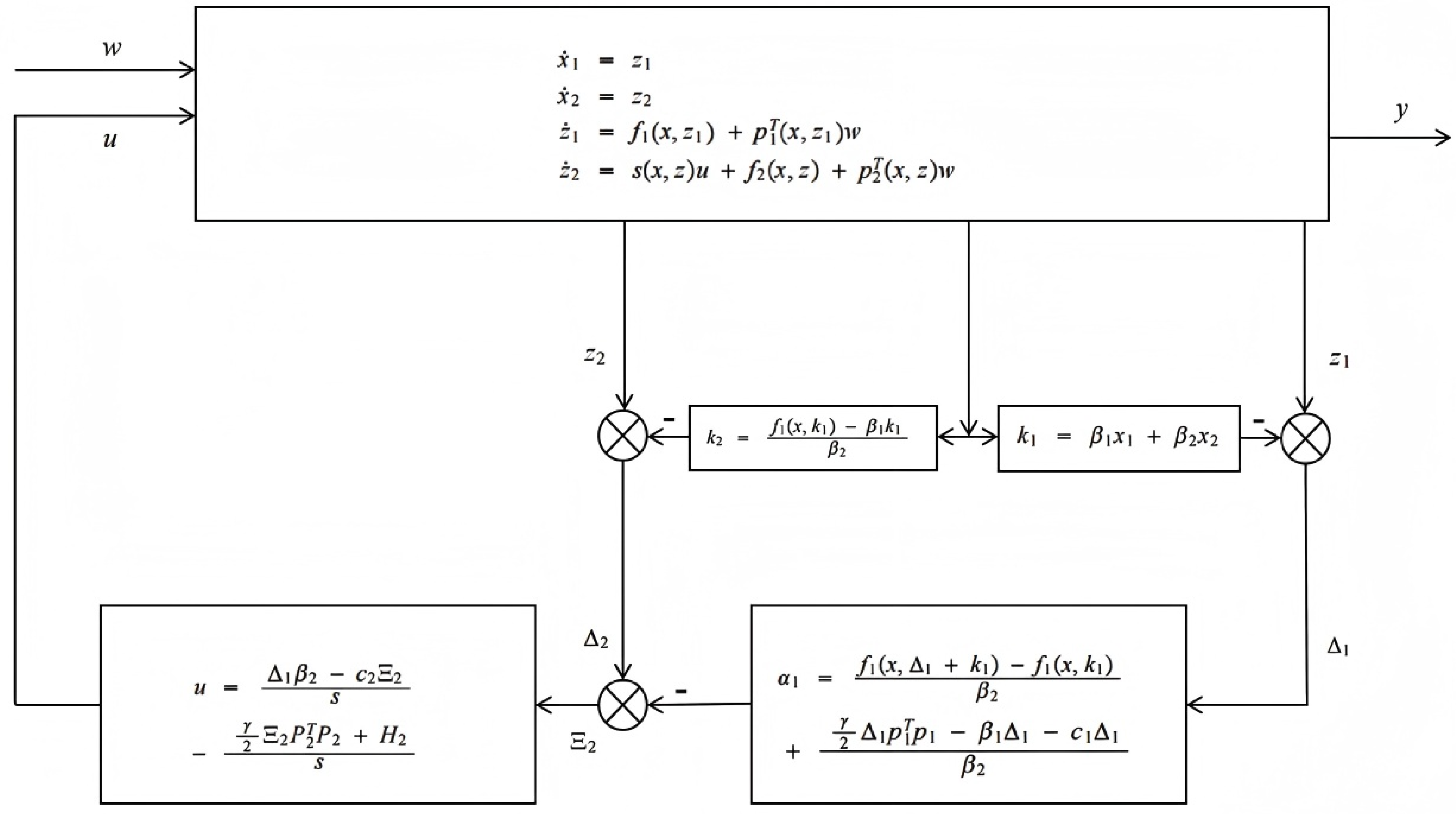
This section is devoted to designing an ADD controller for (1). To this end, a design algorithm is proposed, which is composed of three steps. The first step is to construct a virtual controller so that is stable and satisfies partial differential Equation (7). The second step is to construct a virtual controller to make the derivative of Lyapunov function negative-definite. The third step is to design a controller u. Finally, the local stability of the closed-loop system is theoretically proved based on Lyapunov stability theory. The specific design steps of the controller are given as follows.
Step 1. The following coordinate transformation is introduced.
A virtual controller
is designed such that
is stabilized. In order to eliminate
in
,
satisfies the following PDE:
For simplicity, suppose a solution
satisfies
where
β1 and
β2 are design parameters.
Then, the PDE becomes
which implies that
Then, with (6), the subsystem about
x can be rewritten as
In order to guarantee the stability of (11) with , the following assumption is introduced.
Assumption 2. There exists a function with so that (8) and (9) are satisfied and the origin of (11) with is locally exponentially stable.
Remark 2. According to the converse Lyapunov theorem [35], Assumption 2 implies that there exists a Lyapunov function candidate for subsystem (11) such thatwhere , , , and are positive constants. Step 2. Differentiating (6) yields
where
,
,
is a virtual controller, and
The stability of the closed-loop system is analyzed using Lyapunov’s theorem. A Lyapunov candidate function can be constructed as
Differentiating (18) yields
It follows from Lemma 1 that
Substituting (20) into (19) produces
Therefore,
can be designed as
where
c1 > 0 is a design parameter.
Combining (21) with (22), it can be derived that
With
in (22), (15) can be rewritten as
Step 3. According to (22) and (17),
can be obtained as
where
A Lyapunov candidate
can be introduced as
Differentiating
gives
According to Lemma 1 and (23), Equation (29) can be written as
The controller is shown as follows:
where
c2 > 0 is a design parameter.
Substituting (31) into (30) results in
With u in (31), (25) can be changed to
The design procedure given above can be intuitively visualized with the block diagram in
Figure 1.
Theorem 1. If Assumptions 1 and 2 are satisfied and , , , , λ, and γ are chosen so thatwith the proposed controller (31), the closed-loop system has the following properties: (a) When , the origin of the closed-loop system is locally asymptotically stable.
(b) The following inequality is true:for given and zero initial conditions, , and w satisfying . Proof. Inspired by the proof of Lemma 13.1 in [
36], a Lyapunov function candidate is considered as
where
is a constant. □
The time derivative of
V can be easily expressed as
It follows from Assumption 1 and (22) that
Using Lemma 1 and (14), it follows that
In addition, according to (14) and (40), the following inequality can be easily verified.
Substituting (41) and (42) into (39) produces
According to (13) and (34)–(36), it can be seen that is negative-definite for , which implies that property (a) is true.
To prove the property (b), (46) is rewritten as
Integrating (45) with
gives
which is equivalent to (37) with
.
Remark 3. Note that is the Lyapunov function candidate for subsystem (11) and for subsystem (15) and (25). Therefore, is the Lyapunov function candidate for the whole system composed of two subsystems (11), and (15) and (25).
Remark 4. The challenge of the ADD controller design lies in handling the indefinite term in . Its impact on has to be canceled out by other negative-definite terms through several inequality amplification steps.
4. Simulation Results: Inertia Wheel Pendulum
In this part, the underactuated nonlinear model defined in [
37] for the IWP with a physical damping term satisfying the matching condition is considered to demonstrate the effectiveness of the proposed underactuated ADD backstepping method, which is given by
where
and
stand for the pendulum angle and the disk angle,
and
are the pendulum mass and the wheel mass,
is the distance from the origin to the center of mass of the pendulum,
is the pendulum length,
and
denote the moments of inertia of the pendulum and wheel,
u represents the torque input,
g is the gravity coefficient,
is the damping coefficient, and
and
are disturbances. The IWP system (47) can be rewritten as
where
,
,
, and
.
A new set of variables is defined as
Then, system (48) is changed to (1) with
,
,
,
, and
with
.
The ADD controller for the IWP system is composed of in (8)–(10), in (22), and u in (31).
Remark 5. For this system, can be used so that (12)–(14) are satisfied with , , , , , and due to the following relation.
Remark 6. The region of attraction can be determined by applying the analysis method given in Section 8.2 of the book in [36] to the closed-loop system composed of (11), (24), and (33) with V defined in (38) and . The IWP model parameters taken from [
33] are
kg,
kg,
m,
m,
,
,
, and
. The initial conditions are selected as
rad,
,
, and
. In addition, the controller gains are
,
,
,
, and
.
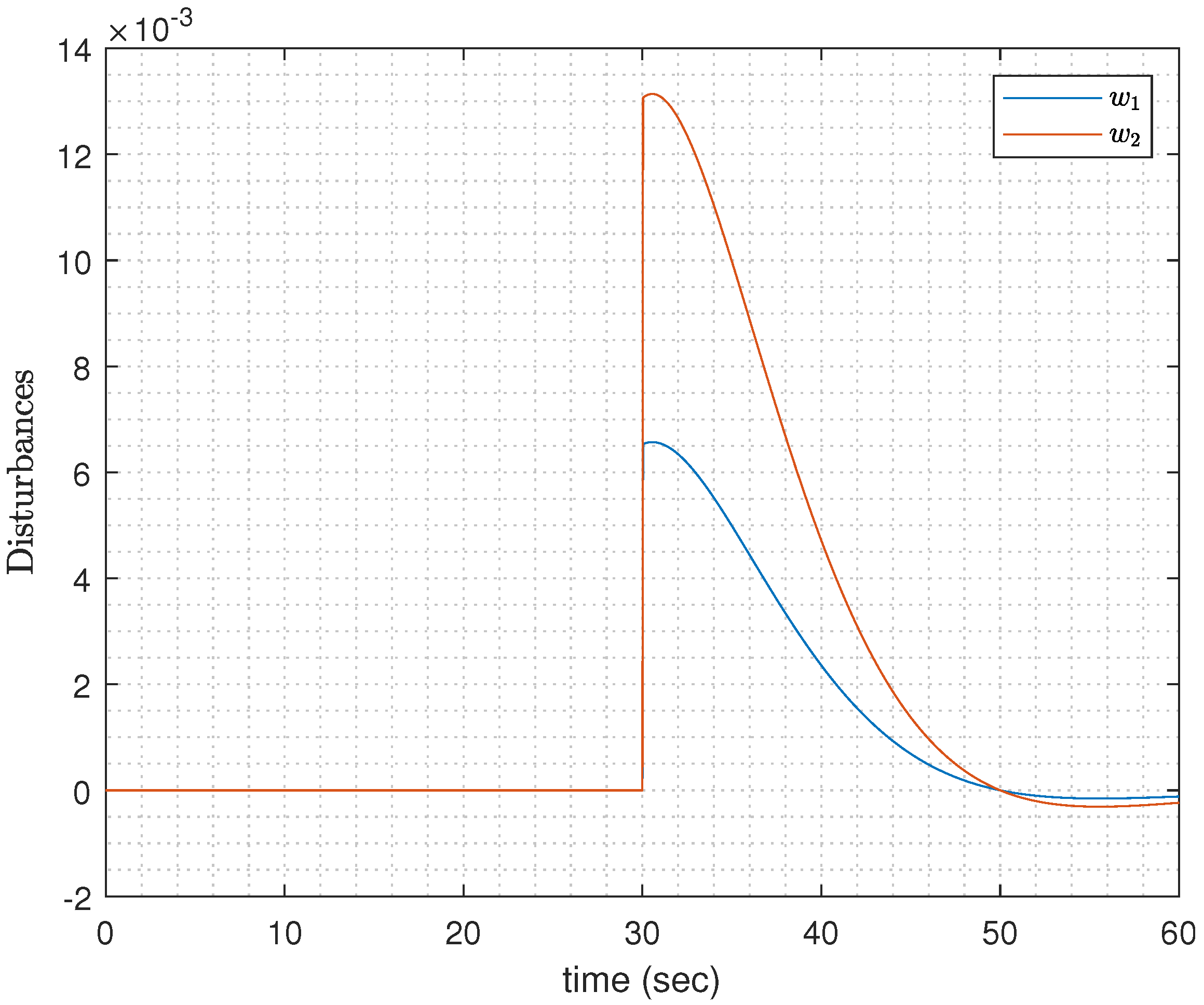
The following disturbances are used in the simulation.
with
and
.
In order to show the superiority of the proposed control method, the feedback linearization method developed in [
28] is simulated on the IWP as well.
The controller in [
28] is given by
where
and
with
,
,
,
,
,
,
, and
.
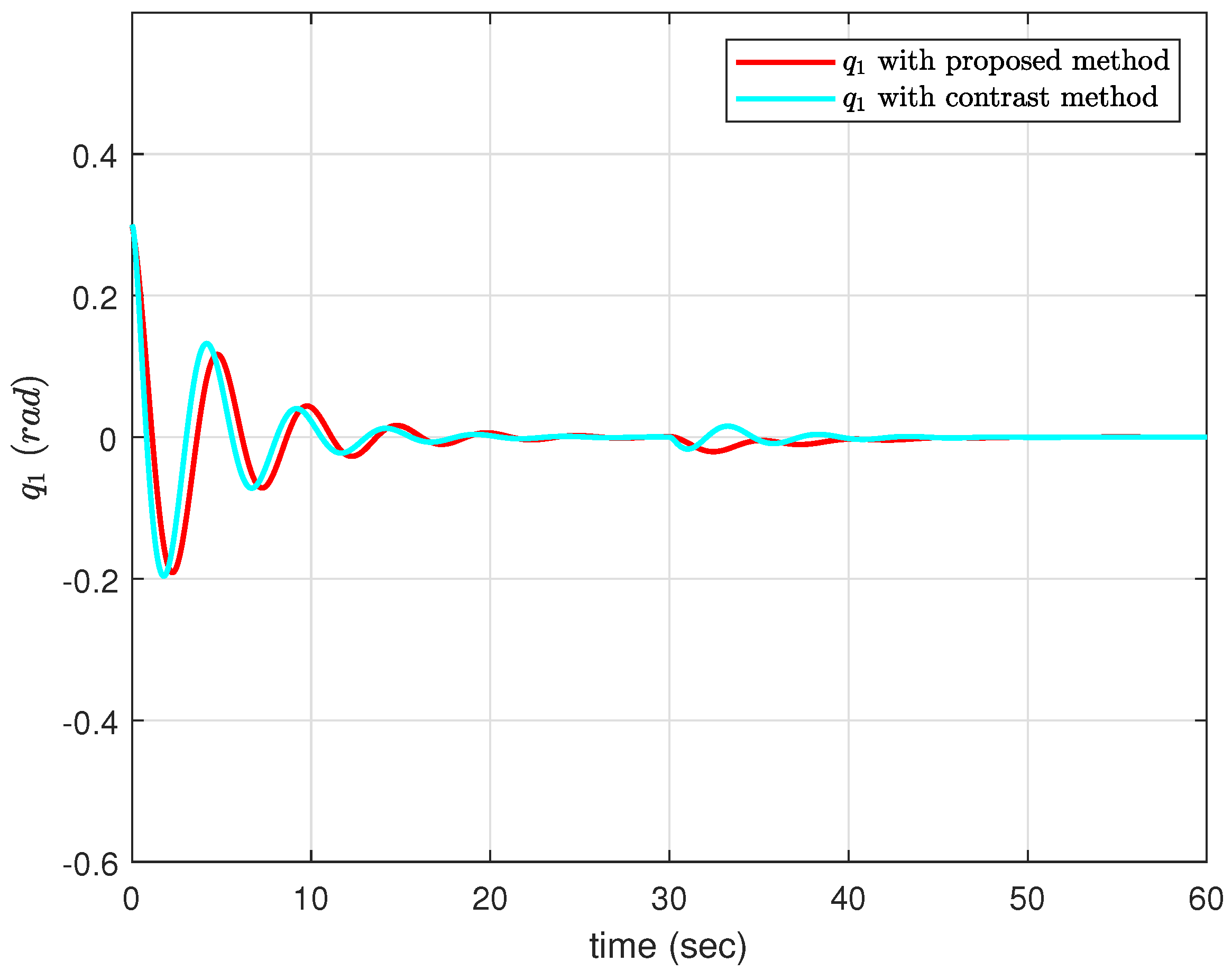
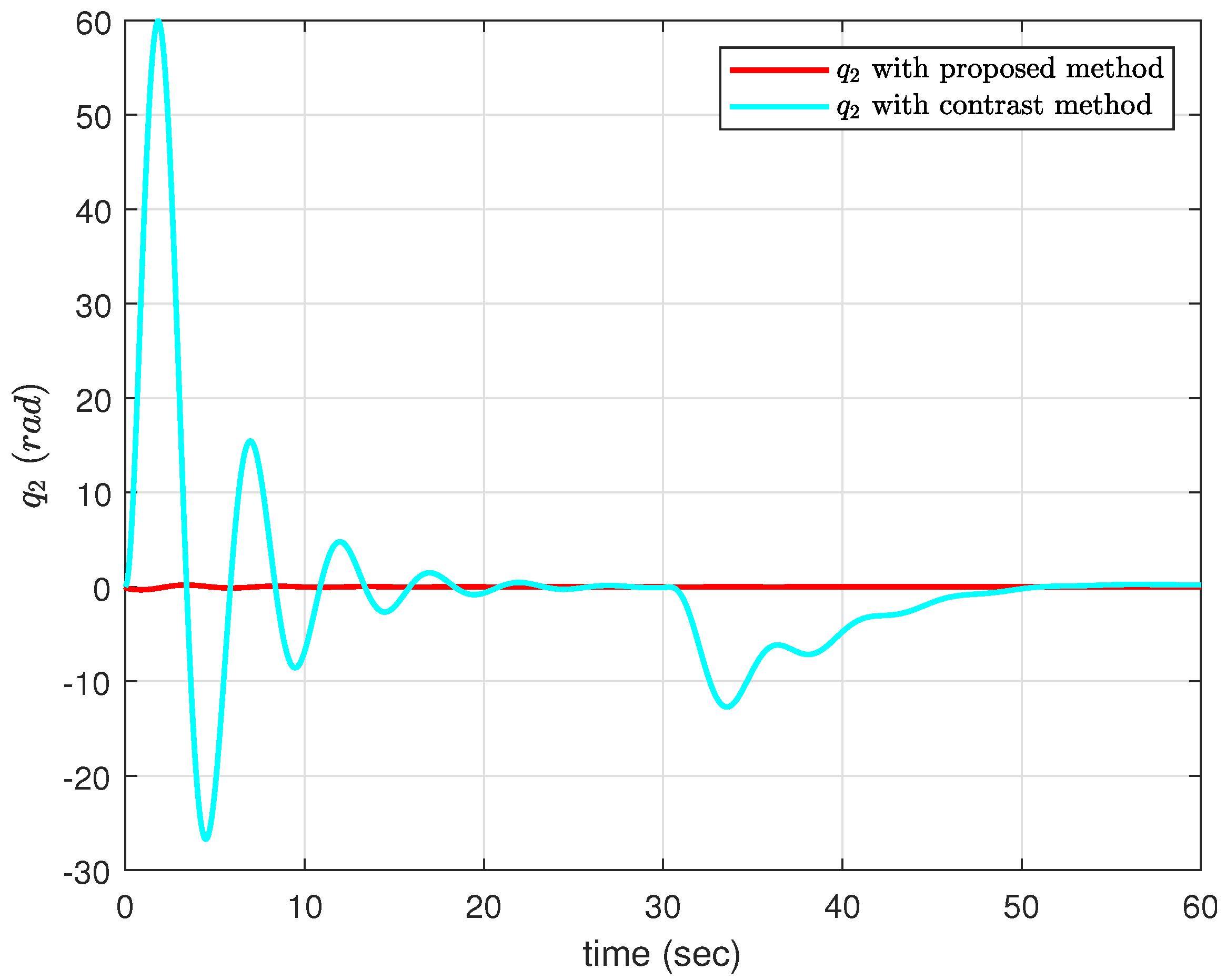
Figure 2,
Figure 3,
Figure 4 and
Figure 5 show the simulation results on the IWP system. As shown in
Figure 2 and
Figure 3, with the proposed method, it takes a shorter time for the IWP to stabilize. After introducing the disturbances (51) at the 30 s mark, which is shown in
Figure 4, the deviation in
with the proposed method is slightly greater than the feedback linearization, while the deviation in
is much smaller compared with the feedback linearization. Furthermore, compared with the proposed method, the feedback linearization experiences much greater oscillation.
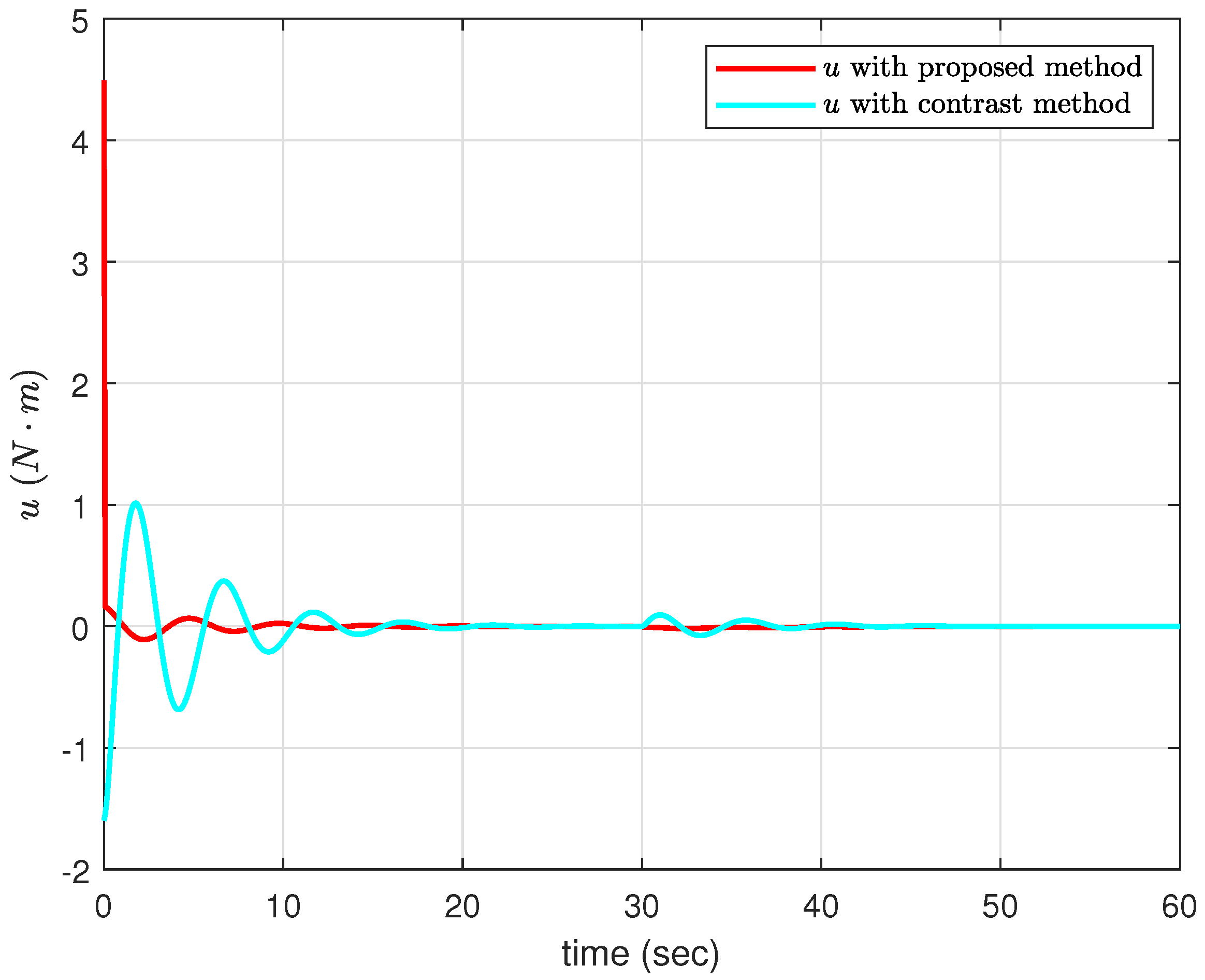
Figure 5 displays the control signals
u. The simulation results of the IWP model validate that the proposed underactuated ADD controller can achieve better control performance compared with the feedback linearization method.
5. Experimental Results: Overhead Crane
This section applies the proposed ADD control algorithm to an overhead crane. The overhead crane can be modeled as
where
and
stand for the trolley displacement and the payload swing angle, respectively;
is the weight of the trolley;
is the weight of the payload;
L is the length of the rope;
g is the gravity coefficient; and
and
are disturbances.
Then, (52) can be linearized at the point
as follows.
where
,
,
,
, and
.
Define
and
. Then,
and
can be expressed as
where
is a desired trolley trajectory and
is a desired swing angle.
A new set of variables is introduced as
Then, by differentiating these variables, system (53) can be changed to (1) with
and
The ADD controller for this overhead crane is composed of in (8) and (10) and in (22) and u in (31).
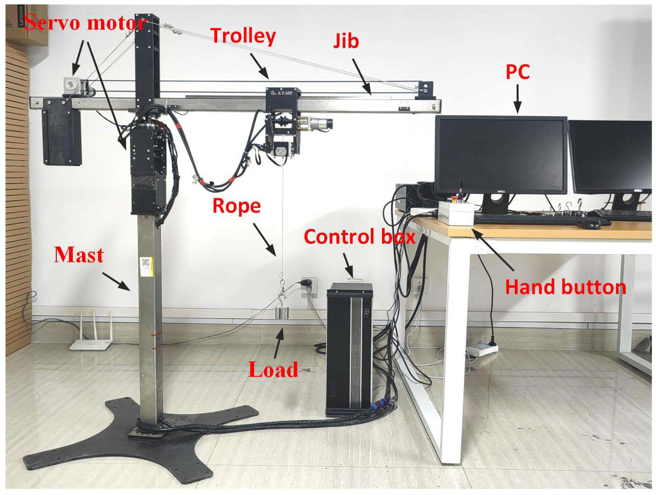
The overhead crane platform is mainly composed of a jib, a trolley, a rope, and a load, as shown in
Figure 6. The platform parameters are
kg,
kg,
m, and
. The controller gains are given below:
,
,
,
, and
. The initial conditions are chosen as
m,
rad,
m/s, and
rad/s.
The proposed ADD controller is applied to control the trolley to track the following reference signal:
where
,
,
,
,
,
,
,
,
,
,
,
with
,
.
The experimental results are presented in
Figure 7,
Figure 8,
Figure 9,
Figure 10 and
Figure 11.
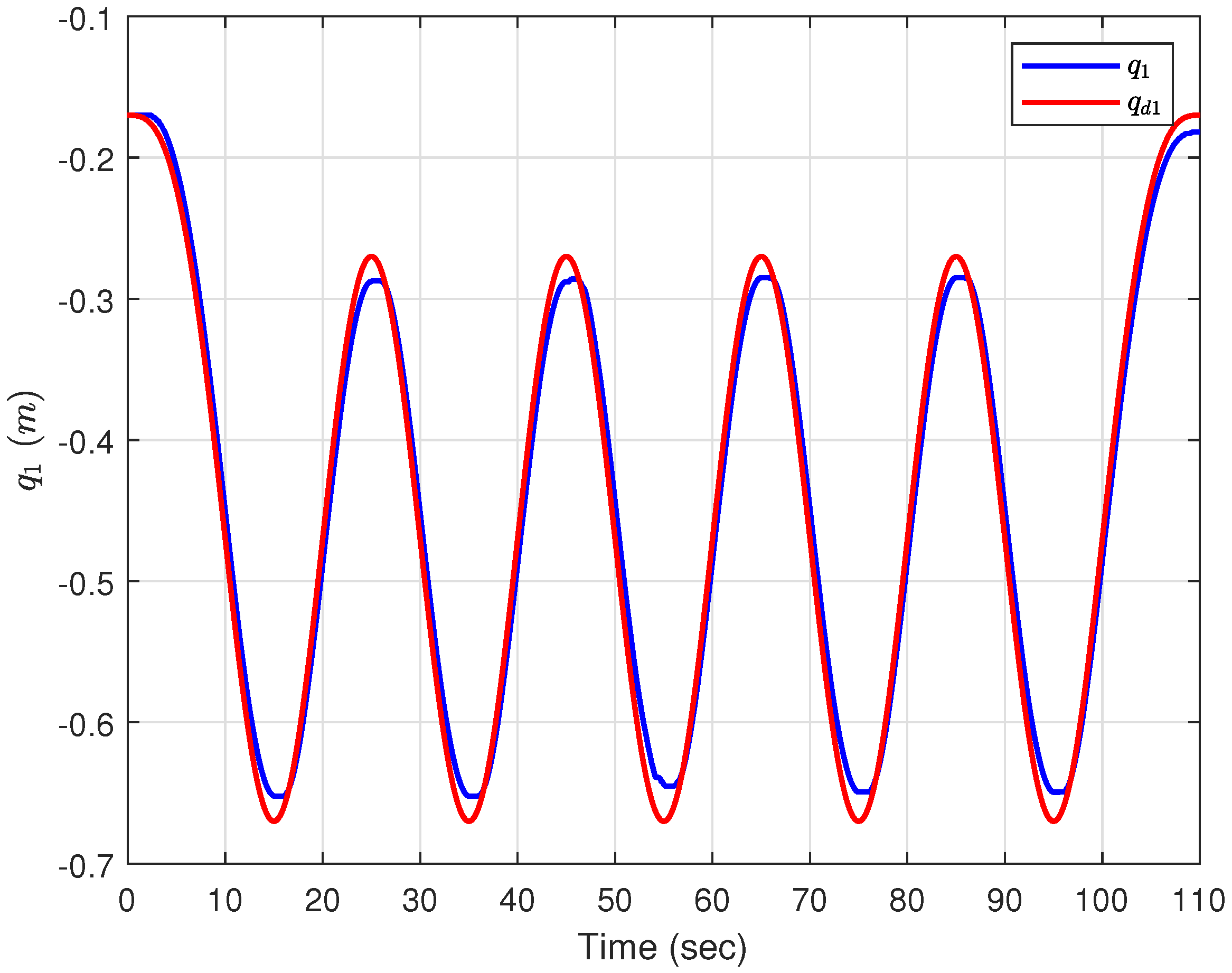
Figure 7 shows the reference and actual trajectories for the trolley, from which it can be observed that the trolley is able to follow the reference trajectory. The tracking error for the trolley is shown in
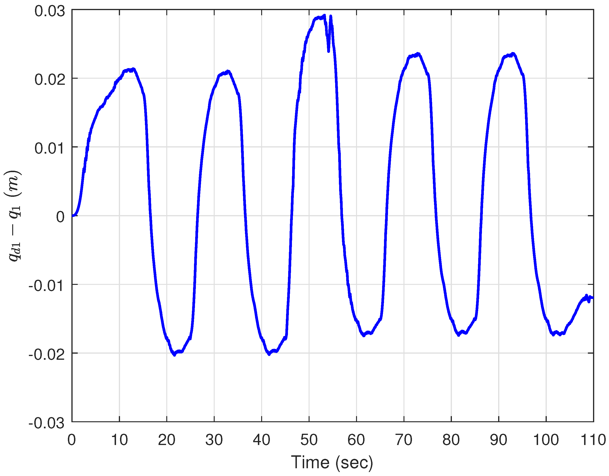
Figure 8.
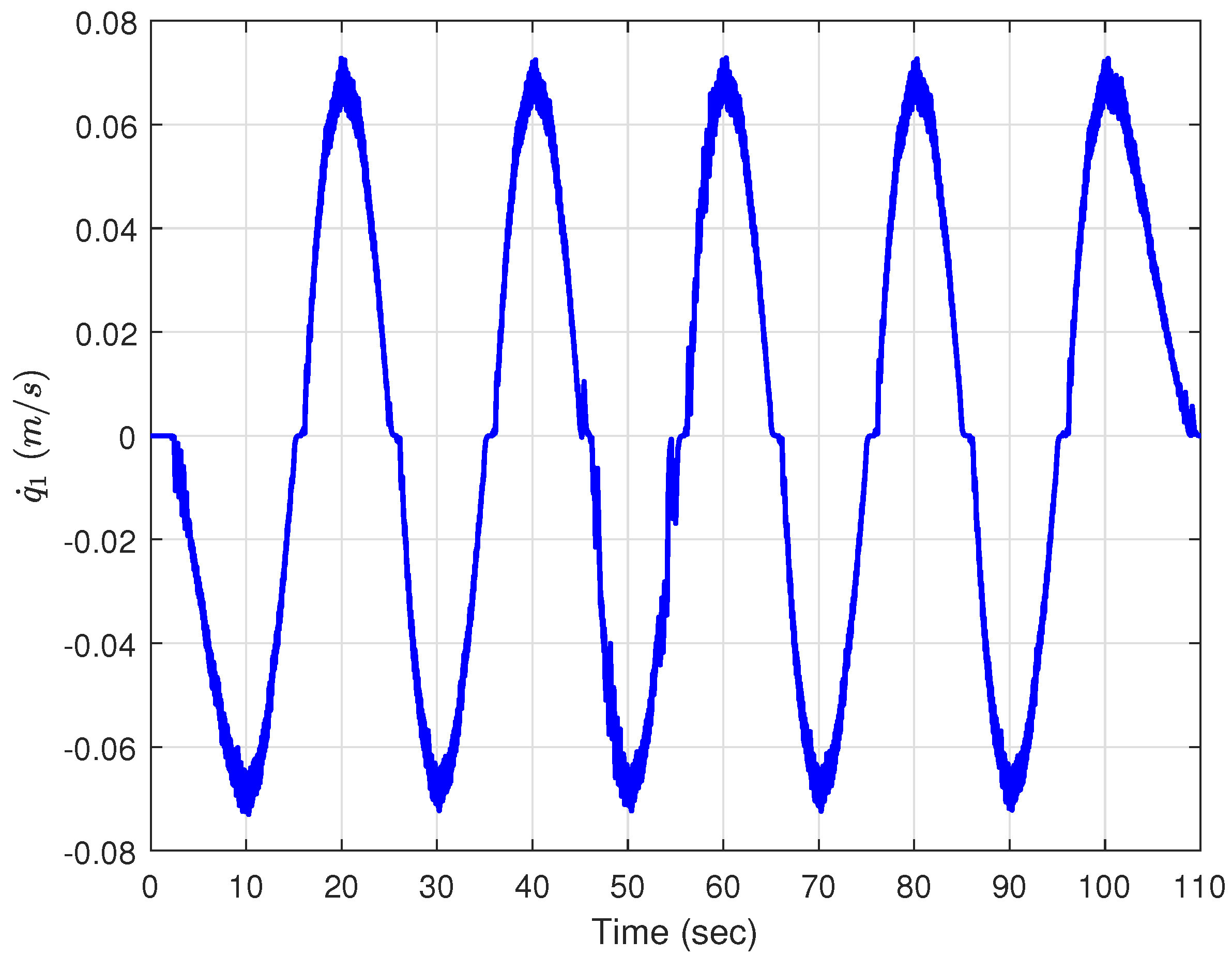
Figure 9 displays the velocity of the trolley.
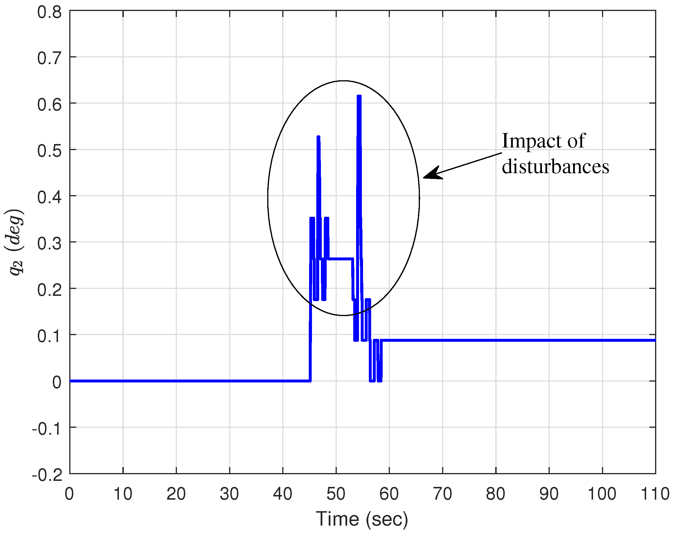
Figure 10 depicts the swinging angle of the payload in the direction of the trolley movement. When disturbances are applied with strong wind from a hairdryer between 45 and 55 s, it can be observed from
Figure 7 and
Figure 10 that the payload experiences some oscillation and quickly returns to its steady-state value and the trolley trajectory is almost unaffected.
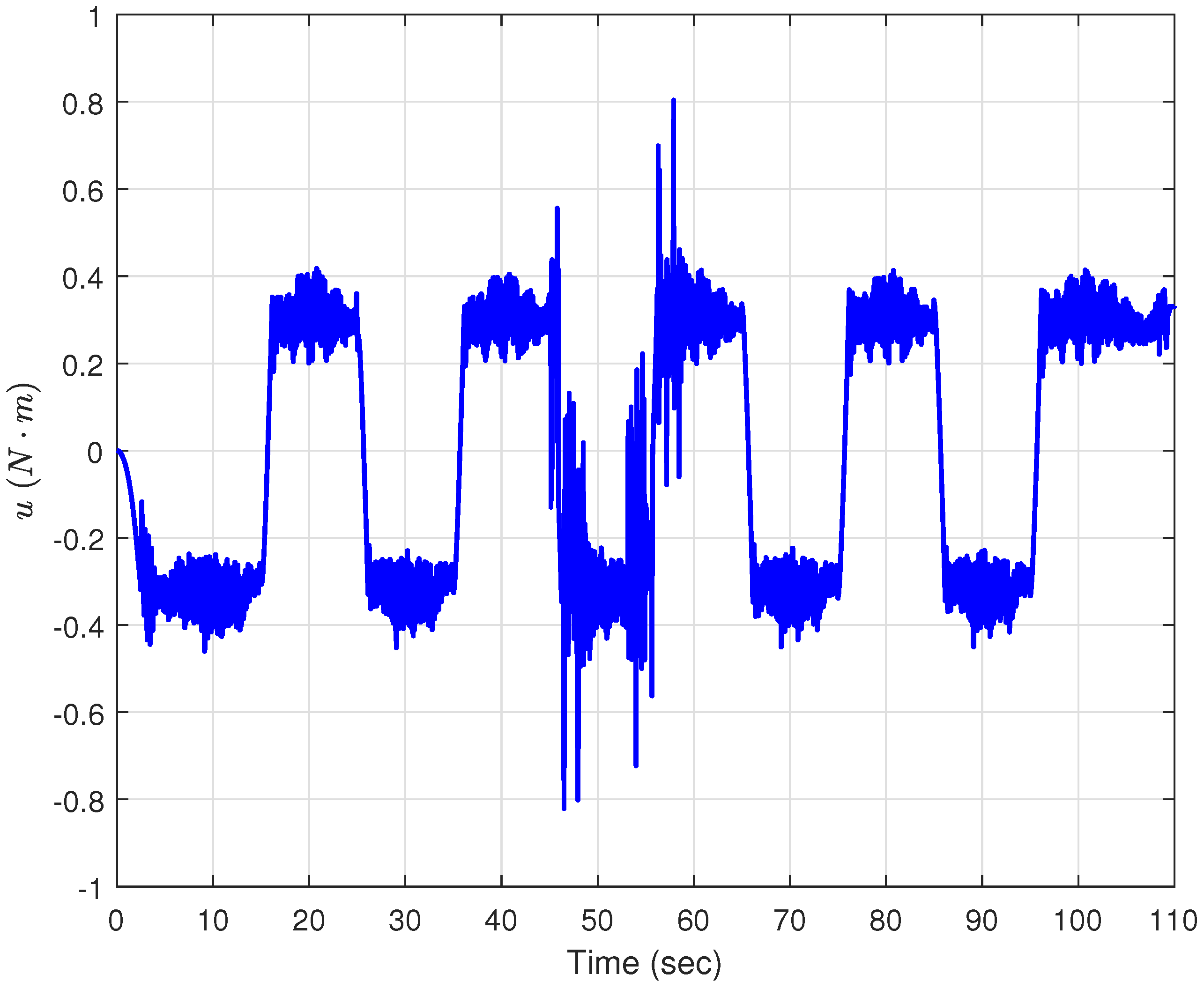
Figure 11 shows that
u is within a reasonable range. Based on the experimental results, it can be concluded that the proposed method is feasible and has a strong disturbance rejection capability.


