Article

Layered and Decoupled Calibration: A High-Precision Kinematic Identification for a 5-DOF Serial-Parallel Manipulator with Remote Drive

1
School of Biomedical Engineering (Suzhou), Division of Life Sciences and Medicine, University of Science and Technology of China, Hefei 230026, China
2
Suzhou Institute of Biomedical Engineering and Technology, Chinese Academy of Sciences, Suzhou 215163, China
*
Author to whom correspondence should be addressed.
Actuators 2025, 14(12), 577; https://doi.org/10.3390/act14120577 (registering DOI)
Submission received: 23 September 2025 / Revised: 25 November 2025 / Accepted: 27 November 2025 / Published: 29 November 2025
(This article belongs to the Section Actuators for Robotics)

Abstract

Serial-parallel hybrid manipulators featuring remote actuation via parallelogram mechanisms are highly valued for their low inertia and high stiffness. However, the complex nonlinear errors introduced by their multi-stage transmission chains pose significant challenges for high-precision calibration. To address this, this paper proposes a hierarchical and decoupled calibration framework specifically tailored for such parallelogram-driven hybrid manipulators. The method first independently calibrates the pose error of the 3-DOF serial main arm using a composite error model that integrates transmission chain constraints. Subsequently, the 2-DOF parallel wrist is accurately calibrated employing a joint-space error identification strategy based on inverse kinematics, thereby circumventing the intractability of solving the parallel mechanism’s forward kinematics. Experimental validation was performed on a self-developed 5-DOF robot prototype using an optical tracker and an attitude sensor. Results from the validation dataset demonstrate that the proposed method reduces the robot’s average positioning error from 2.199 mm to 0.658 mm (a 70.1% improvement) and the average attitude error from 0.8976 deg to 0.1767 deg (an 80.3% improvement). Furthermore, comparative experiments against the standard MDH model and polynomial fitting models confirm that the proposed composite error model and multi-stage transmission error model are essential for achieving high accuracy. This research provides crucial theoretical insights and practical solutions for the high-precision application of complex remote-driven hybrid manipulators.

1. Introduction

Serial manipulators are widely used in industrial applications such as automated welding, assembly, surface painting, and polishing, owing to their large workspace, simple structure, and mature motion control algorithms [1,2,3,4]. Parallel manipulators excel in areas like load capacity, control accuracy, and motion speed, making them prevalent in high-precision scenarios such as precision machining, chip manufacturing, and medical surgery [5,6,7,8,9,10]. However, compared to serial manipulators, the limited workspace of parallel manipulators often limits their utility in broader applications. In this context, the field of robotics has evolved from traditional serial and parallel robots to hybrid manipulators. Current research on hybrid manipulators is primarily divided into two categories: the first combines a low-degree-of-freedom serial mechanism and a parallel mechanism (PM), known as PM + SM (Parallel Manipulator + Serial Manipulator) hybrid manipulators [11,12,13,14,15,16,17]. The second consists of two parallel mechanisms, forming a PM + PM hybrid manipulator [18,19,20]. The five-degree-of-freedom hybrid manipulator studied in this paper, while belonging to the first PM + SM category, employs a multi-level four-bar linkage structure for remote actuation. This makes its control accuracy more difficult to guarantee compared to conventional manipulators. The primary reason lies in the coupling effect of the heterogeneous transmission chain; errors from the serial part are transmitted to the base of the parallel module, while the linkage errors of the serial structure interact with the linkage errors of the parallel structure, ultimately affecting the end-effector output accuracy of the entire system [21,22,23,24,25,26]. This complex interplay of error accumulation and remote actuation makes it extremely challenging to achieve high absolute positioning accuracy. Therefore, precise kinematic parameter calibration has become the key to ensuring end-effector positioning accuracy and promoting its practical application.
Research indicates that approximately 90% of the absolute positioning error in robotic arms originate from kinematic model errors [27]. Consequently, current research on robotic arm calibration primarily focuses on kinematic model-based calibration methods. The objective of this approach is to enhance the absolute positioning accuracy of the robotic arm’s end-effector by identifying and correcting geometric parameter errors caused by factors such as machining, assembly, and wear [28]. The conventional kinematic parameter calibration process comprises four steps: error modeling, external measurement, parameter identification, and error compensation [29,30]. Among these, error modeling is the critical step in kinematic calibration, which uses mathematical tools to establish the error mapping between the robot’s theoretical and actual physical models, thereby providing a foundation for subsequent parameter identification and compensation [31].
However, when modeling robotic arms with non-standard designs, traditional error modeling methods show their limits. The Denavit-Hartenberg (D-H) model is used in traditional robotic arm kinematic modeling to setup geometric errors [32]. The DH model while effective for serial robotic arms, but it causes problems when two joints are parallel to each other. As a result, Hayati et al. suggested an updated DH (MDH) model that adds another parameter to address this [33]. Later models, such as the CPC (Complete and Parametrically Continuous Kinematic) model [34], the POE model [35], and Screw Theory-based models [36,37], have advanced in terms of parameter continuity, completeness, and flexibility. These conventional models predominantly focus on standard open-chain or closed-loop mechanisms, limiting their applicability [38].
The 5-DOF hybrid robotic arm studied herein employs a unique remote-drive design: its drive units are relocated to the base, driving each joint through a multi-stage parallelogram mechanism. This design significantly reduces the arm’s motion inertia while transforming the error model from a simple joint-end-effector mapping into a coupled error system involving the drive-multi-stage transmission-execution chain. For palletizing robots with similar structures, traditional calibration methods for palletizing robotic arms often neglect the nonlinear effects of transmission mechanisms, treating them as simple serial robotic arms [39]. It has been demonstrated that geometric errors introduced by the parallelogram transmission chain constitute a critical error source affecting end-effector precision and cannot be disregarded [40]. Therefore, a high-precision error model must comprehensively reflect the robot’s hybrid configuration by incorporating structural errors from the transmission chain into the overall error system. However, this approach inevitably introduces numerous geometric error parameters, leading to an exceptionally complex model and potentially causing numerical instability and parameter redundancy during parameter identification [41]. Consequently, analyzing error parameters during the modeling stage and eliminating redundant terms is a prerequisite for enhancing identification efficiency and ensuring the reliability of calibration results [42].
This study addresses the aforementioned challenges, and proposes and validates an innovative hierarchical decoupling calibration framework for this type of hybrid robotic arm with parallelogram-based remote drive. The main contributions of this paper include: (1) For the 3-DOF serial main arm, we integrate the serial MDH model with parallel closed-loop constraint equations to establish a hybrid error architecture that coordinates open-chain and closed-chain mechanisms; (2) For the 2-DOF parallel wrist, introducing a joint-space error identification strategy based on inverse kinematics, which circumvents the intractable problem of solving the complex parallel mechanism’s forward kinematics [43]. (3) To quantify the necessity and superiority of the proposed models, designing and executing comprehensive baseline comparisons and ablation studies to quantitatively evaluate the proposed method’s performance against standard MDH models, polynomial-fitting models, and deterministic identification algorithms (LM); (4) To evaluate the model’s robustness, collecting a “stress test” dataset near the mechanism’s singular configurations and analyzing the stability of the identification algorithm (GA).
The remainder of this paper is organized as follows: Section 2 introduces the manipulator architecture and establishes the hierarchical error model. Section 3 presents the error sensitivity analysis. Section 4 details the hierarchical identification and calibration method, defining the baseline models and ablation studies for comparison. Section 5 describes the experimental validation setup, including the planning of calibration, validation, and stress test points. Section 6 provides a detailed report of the calibration results, encompassing performance comparisons against baseline models, robustness stress testing, and algorithm stability analysis. Finally, Section 7 offers a conclusion and outlook.

2. Configuration Design and Hierarchical Error Modeling

2.1. Configuration Design

The virtual prototype and schematic diagram of the self-developed 5-DOF hybrid robotic arm are shown in Figure 1. As depicted in Figure 1a, the robotic arm consists of a 3-DOF serial main arm and a 2-DOF parallel wrist, facilitating three-dimensional spatial positioning and two-directional orientation adjustment at the end effector. A distinguishing design feature is the employment of a multi-stage parallelogram mechanism for remote actuation. All drive units are consolidated at the robot base to reduce motion inertia and enhance rigidity.
The kinematic configuration of the serial main arm is shown in Figure 1b. It comprises the base rotation joint ( θ 1 ), the main arm pitch joint ( θ 2 ), and the forearm pitch joint ( θ 3 ). The actuation for the forearm joint ( θ 3 ) is transmitted via a set of parallelogram mechanisms on the main arm (L-K-P-E in Figure 1b).
The topology of the parallel wrist is shown in Figure 1c. It comprises a moving platform (with its origin at F 1 ) and a stationary platform rigidly connected to the end of the serial arm. These two platforms are connected by two identical, symmetrically arranged RUS (Revolute-Universal-Spherical) kinematic chains. Here, R 1 and R 2 are active revolute joints located on the stationary platform. Their rotation drives the moving platform to achieve two-dimensional rotation around the x- and y-axes. The active joints R 1 and R 2 of the wrist are also remotely driven by independent, multi-stage parallelogram transmission chains originating from the base. Their multi-stage transmission path is shown in Figure 2b.
To clearly establish the kinematic and error models, Table 1 lists the nominal kinematic parameters of the manipulator. These design dimensions form the basis for subsequent error models and sensitivity analyses. Here, l s represents the nominal dimension of the four-bar linkage of the serial main arm, and l p 1 ~ l p 4 represent the nominal dimensions of each stage of the parallel wrist linkage from the base position to the parallel wrist.

2.2. Hierarchical Error Modeling

This section establishes distinct error models for the 3-DOF serial main arm and the 2-DOF parallel wrist to underpin the DOF-based error decoupling calibration technique suggested in this paper. Additionally, the impact of linkage parameter inaccuracies from the individual parallelogram mechanisms on these models will be considered.

2.2.1. Error Modeling of Parallelogram Transmission

In the design of the 5-DOF hybrid manipulator, parallelogram mechanisms are integral components of the transmission chains for both the 3-DOF serial main arm and the 2-DOF parallel wrist. Their main purpose is to facilitate a remote drive design where actuators are mounted at the base, and torque is delivered to the respective joints via one or more stages of parallelogram linkages. This configuration serves to decrease the manipulator’s moving mass and overall inertia. Nevertheless, this design also introduces complex and nonlinear sources of error. In particular, kinematic errors arising from inaccuracies in link lengths and misalignments in passive joints are directly propagated to the end-effector, thereby degrading its final pose accuracy.
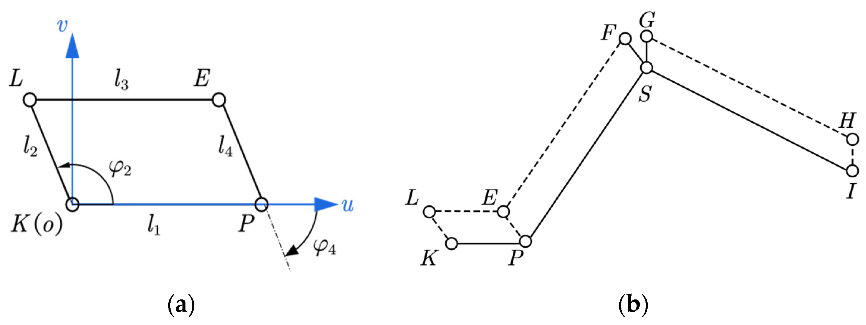
Figure 2 illustrates the multi-stage parallelogram transmission chain used for the remote actuation of the 2-DOF parallel wrist. We begin by formulating an error model for the initial parallelogram linkage of this chain, LEPK (as shown in Figure 2a). The input terminal K of this linkage is rigidly connected to the output shaft of a base-mounted actuator. The output rotation from this parallelogram is then progressively transmitted through subsequent linkages (as shown in Figure 2b) to the final joint of the wrist.
As shown in Figure 2a, the First-stage parallelogram mechanism forms the L-E-P-K closed loop, which consists of the fixed link l 1 , the driving link l 2 , the coupler link l 3 , and the output link l 4 . Under ideal conditions, this mechanism behaves as a perfect parallelogram, meaning φ 2 = φ 4 , where φ 2 is the angle of the driving link and φ 4 is the angle of the output link. However, to account for manufacturing and assembly errors, it must be modeled as a general four–bar linkage. A planar Cartesian coordinate system, o–uv, is established with its u–axis aligned with the fixed link l 1 . The lengths of the links are denoted by l 1 , l 2 , l 3 , and l 4 , and their respective angles with the u–axis are φ 1 , φ 2 , φ 3 , and φ 4 . The corresponding complex number representation for each link is therefore l 1 e j φ 1 , l 2 e j φ 2 , l 3 e j φ 3 , and l 4 e j φ 4 .
Since the four–bar linkage forms a closed kinematic loop, its vector loop equation in the complex plane can be established for the LEPK linkage as:
k = 1 4 l k e j φ k = 0
To analyze the sensitivity of the output link’s angle to small geometric errors, we take the total differential of the vector expression for each link, yielding:
d d t l k e j φ k = Δ l k e j φ k + j l k Δ φ k e j φ k
Summing the differential terms for all four links gives the error loop equation:
k = 1 4 Δ l k e j φ k + j l k Δ φ k e j φ k = 0
To facilitate the subsequent derivation, all terms in Equation (3) are projected onto a reference frame aligned with the direction of link l 3 (i.e., angle φ 3 ). This is achieved by multiplying both sides of Equation (3) by e j φ 3 and then taking the real part, which results in:
k = 1 4 Δ l k c o s φ k φ 3 l k Δ φ k s i n φ k φ 3 = 0
Since Link 2 is the driving link, we assume its angular error is zero (i.e., φ 2 = 0 ), as it serves as the input reference. For an ideal parallelogram mechanism, the following geometric relationships between the link lengths and angles must be satisfied:
l 1 = l 3 , l 2 = l 4 , φ 1 = π , φ 4 = π + φ 2
Substituting these relationships into Equation (4), the expression for the output angle error, φ 4 , is obtained as:
Δ φ 4 = c o s φ 2 Δ l 2 Δ l 4 + Δ l 3 Δ l 1 l 2 s i n φ 2
To simplify the subsequent analysis, the four individual link length errors are consolidated into two terms representing the differences in opposing link lengths: the driving–side error, l s = l 2 l 4 , and the transmission–side error, l t = l 3 l 1 . The error function can thus be expressed in a more compact form with the input angle φ 2 and these error difference terms as variables:
Δ φ 4 = f φ 2 , Δ l s , Δ l t = Δ l s c o s φ 2 + Δ l t l 2 s i n φ 2
Equation (7) clearly reveals the nonlinear mapping between the output angle error, φ 4 , and the input angle, φ 2 . The denominator, l 2 s i n φ 2 , approaches zero as φ 2 approaches the singular configurations of 0 or π. In these regions, the system becomes highly sensitive to geometric errors, leading to a singular response. Therefore, the operational workspace of the driving angle must be designed to avoid these sensitive regions.
For a multi–stage transmission chain composed of serially connected four-bar linkages, each stage transmits the angle from the previous stage to the next while introducing an additional angular error. These errors accumulate and are ultimately reflected in the final output angle. It is therefore necessary to establish a general error model for such multi-stage structures. For the n-th stage in the chain, let the input angle be φ n _ i , the output angle be φ n _ o , and the angular error induced by its link length imperfections be Δ φ n . This error depends on the link error terms and the input angle of the current stage, expressed as:
φ n _ o = φ n _ i + Δ φ n = φ n _ i + f φ n _ i , Δ l s , Δ l t
where l n _ s = l n _ 2 l n _ 4 is the driving-side error term for the n-th stage, and l n _ t = l n _ 3 l n _ 1 is the transmission-side error term. The input angle of each stage is determined by the output of the previous stage, following this recursive relationship:
φ n _ i = φ n 1 _ o = φ n 1 _ i + φ n 1 n = 1,2 ,
This model captures the nonlinear and coupled characteristics of the errors within the transmission chain. The error at any given stage is influenced not only by its own geometric parameters but also by the accumulated errors propagated from all preceding stages. This formulation lays the groundwork for the subsequent sensitivity analysis and error compensation.
It should be noted that the model established by Formulas (7) and (9) is a kinematic model, which mainly focuses on the geometric dimensional errors (i.e., link length errors Δ l s , Δ l s ) caused by manufacturing and assembly tolerances. This model assumes that all links are rigid bodies and does not consider nonlinear dynamic effects such as elastic deformation, joint clearance, or friction under load. This is because, under low-speed, light-load calibration conditions, geometric errors caused by tolerances are usually the dominant factors leading to deviations in the accuracy of the robotic arm’s end effector. Therefore, this study focuses on identifying and compensating for these first-order geometric errors, which is critical for improving the manipulator’s absolute positioning accuracy.

2.2.2. Error Kinematic Modeling of the 3-DOF Serial Main Arm

This section establishes an error kinematic model for the first 3-DOF serial main arm of the hybrid manipulator. This part consists of three joints: the base revolute joint, the main arm revolute joint, and the forearm revolute joint, forming a typical 3-DOF serial structure. Under ideal modeling conditions, its forward kinematics can be modeled using the D-H method. The D-H transformation matrix can be expressed as:
T i i 1 = Rot z , θ i Trans z , d i Trans x , a i Rot x , α i = c θ i s θ i c α i s θ i s α i a i c θ i s θ i c θ i c α i c θ i s α i a i s θ i 0 s α i c α i d i 0 0 0 1 , i = 1,2
However, the traditional D-H model can exhibit singularities when adjacent joints are parallel or nearly parallel, and its representation of parameter perturbations is not continuous. Therefore, when there are two consecutive parallel joints, a five-parameter MDH model is adopted, which introduces an additional y-axis rotation. Its MDH transformation matrix can be expressed as:
T i i 1 = Rot z , θ i Trans z , d i Trans x , a i Rot x , α i Rot y , γ i = c θ i c β i s θ i s α i s β i s θ i c α i c θ i s β i + s θ i s α i s β i a i c θ i s θ i c β i + c θ i s α i s β i c θ i c α i s θ i s β i c θ i s α i c β i a i s θ i c α i s β i s α i c α i c β i d i 0 0 0 1 ,   i = 3
where the five MDH parameters are defined as:
β i : the initial correction angle around the y-axis (to compensate for initial mechanism offsets).
θ i : the joint variable, corresponding to the rotation angle around the z-axis.
d i : the link offset, corresponding to the translation along the z-axis.
a i : the link length, corresponding to the translation along the x-axis.
α i : the link twist, the angle between adjacent z-axes measured about the common X-axis.
When introducing error modeling, we consider that the link parameters have small perturbations. Let the geometric parameter deviation vector for the i-th link be e i =   [ Δ θ i , Δ d i , Δ a i , Δ α i , β i ] , and the manipulator’s overall error vector be e = [ e 1 , e 2 , e 3 ] . The joint variables are q = [ θ 1 , θ 2 , θ 3 ] . The third joint of the 3-DOF serial main arm is driven by a parallelogram mechanism. As can be seen from the schematic diagram in Figure 1, its joint angle, θ 3 , is the same as the output angle of the parallelogram, φ 2 . From Equation (7), it is known that the opposing-side length error l = [ l s , l t ] of the parallelogram will cause an angular error of φ 4 for θ 3 .
According to the theory of homogeneous transformations, the error mapping matrix from the manipulator’s base coordinate system can be expressed as:
T ( q , e ) 3 0 = T ( e 1 ) 1 0 T ( e 2 ) 2 1 T ( e 3 , l ) 3 2 = r p 0 1
For i = 1, 2:
T ( e i ) i i 1 = R o t z i , θ i + Δ θ i T r a n s z i , d i + Δ d i T r a n s x i , a i + Δ a i R o t x i , α i + Δ α i
For i = 3:
T ( e 3 ) 2 3 = R o t z 3 , θ 3 + Δ θ 3 + Δ φ 4 T r a n s z 3 , d 3 + Δ d 3 T r a n s x 3 , a 3 + Δ a 3 R o t x 3 , α 3 + Δ α 3 R o t y 3 , β 3 + Δ β 3
Equation (12) can be expressed as a mapping relationship between the position vector p, the joint variables q, and the parameter error set e, as follows:
p = F ( q , e )
where the mapping function F represents the complete kinematic error model of the 3-DOF serial main arm, and e is the set of all its geometric parameter errors. For the forearm joint, the model explicitly includes the angular error φ 4 , which is propagated from the parallelogram transmission mechanism and is defined in Equation (7). Therefore, the error modeling for this hybrid serial-parallel structure not only encompasses the deviations in nominal geometric link parameters but also accounts for the error propagation path from the internal transmission mechanism. This comprehensive model forms the basis for the subsequent sensitivity analysis and parameter identification.

2.2.3. Error Kinematic Modeling of the 2-DOF Parallel Wrist

Figure 3a shows the Virtual prototype of the 2-DOF parallel wrist. For descriptive convenience, the model is simplified into a kinematic diagram as shown in Figure 3b. As can be seen from Figure 3b, the 2-DOF parallel wrist at the end consists of a moving platform ( F 1 , S 1 , S 2 ) and two identical RUS kinematic chains ( R 1 - U 2 - S 1 and R 1 - U 3 - S 2 ) on the left and right sides. In the diagram, ‘U’ represents a universal joint, ‘R’ a revolute joint, and ‘S’ a spherical joint. The two revolute joints, R 1 and R 2 , serve as the base points for the two kinematic chains. The mechanism is actuated by the multi-stage parallelogram transmission chains on either side of the manipulator, which drive the rotation of R 1 and R 2 to achieve the 2-DOF rotation of the terminal parallel mechanism about the x- and y-axes.
Let q 1 and q 2 be the rotation angles of the cranks R 1 U 2 and R 2 U 3 about the R 1 R 2 axis, respectively. It is defined that when the cranks R 1 U 2 and R 2 U 3 are horizontal, q 1 = q 2 = 0. The plane U 1 U 2 U 3 constitutes the stationary platform, where
U 1 U 2 = U 1 U 3 = F 1 S 1 = F 1 S 2 R 1 R 2 = S 1 S 2 = U 2 U 3
As shown in Figure 3b, coordinate systems for the parallel mechanism are established. The origins of the stationary and moving platform coordinate systems are defined as o 4 and o 5 , respectively. The origin o 4 is located at the midpoint of the R 1 R 2 line segment. When the joint angles q 1 and q 2 are zero, the o 5 coordinate system is positioned directly above the o 4 coordinate system. The angles γ and β represent the rotation of the moving platform about the x 4 - and y 4 -axes, respectively. In this home pose, both the input and output angles are zero. For descriptive convenience, we make the following conventions:
R 1 R 2 = S 1 S 2 = U 2 U 3 = r R 1 U 2 = R 2 U 3 = s S 1 U 2 = S 2 U 3 = F 1 U 1 = u
In the coordinate frame o4, the coordinates of points U 1 , U 2 , and U 3 are expressed as:
U 1 4 = 0 ,   0 ,   0 U 2 4 = s c q 1 , r 2 ,   s s q 1 U 3 4 = s c q 2 ,   r 2 ,   s s q 2
In the coordinate frame o5, the coordinates of points U 1 , U 2 , and U 3 are expressed as:
F 1 5 = 0 ,   0 ,   0    S 1 5 = s ,   r 2 ,   0 S 2 5 = s ,   r 2 ,   0
The transformation matrix from frame o4 to frame o5, T54, for an x-y-z fixed-angle rotation sequence, is given by:
T 45 = R 45 P 45 0 1 = c β s β s γ s β c γ x 45 0 c γ s γ y 45 s β c β s γ c β c γ z 45 0 0 0 1
where the vector P45 = [x45, y45, z45]T represents the coordinates of the origin of frame o5 expressed in the stationary frame o4. The inverse transformation, T54, is obtained as:
T 54 = R 45 T P 54 0 1 = c β 0 s β x 45 c β z 45 s β s β s γ c γ c β s γ x 45 s β s γ + y 45 c γ + z 45 c β s γ s β c γ s γ c β c γ x 45 s β c γ y 45 s γ + z 45 c β c γ 0 0 0 1
Using the transformation from frame o4 to o5, the coordinates of the universal joint U 1 can be expressed in frame o5:
U 1 5 = T 54 U 1 4
Since the point U 1 on the stationary platform has a fixed position relative to the moving frame o4, its coordinates in frame o5 are constant, given by P54 = [0, 0, −u]. By substituting this into the equation above and combining it with Equation (21), the relationships can be simplified:
0 = x 45 c β + z 45 s β 0 = x 45 s β s γ y 45 c γ z 45 c β s γ u = x 45 s β c γ + y 45 s γ z 45 c β c γ x 45 = u s β c γ y 45 = u s γ z 45 = u c β c γ
Substituting these simplified relations back into Equation (20), we obtain the updated transformation matrix T45:
T 45 = c β s β s γ s β c γ u s β c γ 0 c γ s γ u s γ s β c β s γ c β c γ u c β c γ 0 0 0 1
Using the transformation matrix T45 from frame o5 to frame o4, the coordinates of the spherical joint S 1 , S 2 in frame o4 can be obtained as follows:
S 1 4 = T 45 S 1 5 = s c β r 2 s β s γ + u s β c γ r 2 c γ u s γ s s β r 2 c β s γ + u c β c γ S 2 4 = T 45 S 2 5 = s c β + r 2 s β s γ + u s β c γ r 2 c γ u s γ s s β + r 2 c β s γ + u c β c γ
Since the distance between the universal joint and the spherical joint is constant and equal to u, applying the distance formula between these two points gives:
S 1 4 U 2 4 = sc β r 2 s β s γ   +   us β c γ sc q 1 2 + r 2 c γ us γ   +   r 2 2 + ss β r 2 c β s γ   +   uc β c γ ss q 1 2 = u S 2 4 U 3 4 = sc β   +   r 2 s β s γ   +   us β c γ sc q 2 2 + r 2 c γ us γ r 2 2 + ss β   +   r 2 c β s γ   +   uc β c γ ss q 2 2 = u
Equation (26) can be simplified to:
  K 11 c q 1 + K 12 s q 1 = K 13 K 21 c q 2 + K 22 s q 2 = K 23
where the coefficients K 11 , K 12 , K 13 , K 21 , K 22 , K 23 , are functions of γ and β, with their specific expressions given by:
K 11   =   rss β s γ     2 s 2 c β     2 uss β c γ K 12   =   rsc β s γ   +   2 s 2 s β     2 usc β c γ K 13 =   r 2 c γ 2     r 2 2   +   rus γ     2 s 2 K 21 = rss β s γ     2 s 2 c β     2 uss β c γ K 22 = rsc β s γ   +   2 s 2 s β     2 usc β c γ K 23 =   r 2 c γ 2     r 2 2     rus γ     2 s 2
By applying the tangent half-angle substitution, the joint variables q 1 and q 2 are reparameterized as:
u 1 = t a n q 1 2 u 2 = t a n q 2 2
It follows that the sine and cosine terms can be expressed as:
s i n q 1 = 2 u 1 1 + u 1 2 ,   s i n q 2 = 2 u 2 1 + u 2 2 c o s q 1 = 1 u 1 2 1 + u 1 2 ,   c o s q 2 = 1 u 2 2 1 + u 2 2
Substituting these expressions into Equation (27) yields:
K 11 1 u 1 2 1 + u 1 2 + K 12 2 u 1 1 + u 1 2 = K 13 K 21 1 u 2 2 1 + u 2 2 + K 22 2 u 2 1 + u 2 2 = K 23
Equation (31) can be simplified and rearranged to obtain:
K 11 + K 13 u 1 2 2 K 12 u 1 + K 13 K 11 = 0 K 21 + K 23 u 2 2 2 K 22 u 2 + K 23 K 21 = 0
The solution to Equation (32) is discussed on a case-by-case basis:
Case 1: When K 11 + K 13 0 , K 11 + K 13 0 , the expressions in (32) are quadratic equations. Solving for u 1 and u 2 yields:
u 1 = K 12 ± K 11 2 + K 12 2 K 13 2 K 11 + K 13 u 2 = K 22 ± K 21 2 + K 22 2 K 23 2 K 21 + K 23
Case 2: When K 11 + K 13 = 0 , K 11 + K 13 = 0 , the expressions in (31) degenerate into linear equations. The solutions are:
u 1 = K 13 K 11 2 K 12 u 2 = K 23 K 21 2 K 22
By combining the solutions from both cases and reversing the tangent half-angle substitution, the joint angles q 1 and q 2 are found as:
q 1 = a r c t a n 2 u 1 1 u 1 2 q 2 = a r c t a n 2 u 2 1 u 2 2
The derivation above establishes the inverse kinematic model for the parallel wrist. Due to the inherent complexity of parallel mechanisms, closed-form analytical solution often does not exist for their forward kinematics. Simplifying Equation (26) results in a transcendental equation simultaneously involving γ and β, which cannot be solved analytically. Consequently, it is infeasible to establish a mapping between the pose error in the o5 coordinate frame and the parameter error of the parallel mechanism. This limitation presents a significant bottleneck for traditional calibration methods that rely on end-effector pose errors. To address this issue, this section proposes an innovative joint-space error calibration strategy based on the inverse kinematics model. The core idea of this method is to avoid establishing a mapping between geometric parameter errors and end-effector pose errors. Instead, it utilizes the derived closed-form inverse kinematics model to establish a mapping between geometric parameter errors and driven joint angle errors, thereby circumventing the intractable problem of solving the forward kinematics model.
Ideally, Pn represents the nominal design values of the kinematic parameters for the 2-DOF parallel mechanism. However, due to manufacturing and assembly errors, the actual geometric parameters will deviate from their nominal values. Let p be the set of these structural parameter errors. When the precise actual orientation of the terminal moving platform, x m = γ m , β m , is acquired via an external measurement device, and the corresponding actual angles of the actuated joints, q m = q m 1 , q m 2 , are measured simultaneously, the mapping relationship between the actuated joint angles, the moving platform’s orientation, and the parameter error set can be derived from Equations (27)–(35) as follows:
q m = F γ m , β m , P a = F x m , P n + Δ P
The mapping function F represents the kinematic error model of the parallel mechanism.
Similar to the transmission chain model, the parallel wrist inverse kinematic error model established by Equation (36) is also based on the rigid body assumption. This model aims to identify the geometric parameter errors of the mechanism (such as Δ s , Δ r ), but does not yet include factors such as elastic deformation or joint clearance. This simplification is reasonable and effective for kinematic calibration under quasi-static conditions, and its focus is on correcting geometric error sources caused by manufacturing and assembly tolerances.

3. Sensitivity Analysis and Parameter Identification

In Section 2, a composite error model was established for the 5-DOF hybrid manipulator, which incorporates the serial main arm, the parallel wrist, and the multi-stage transmission chains. This model contains a large number of geometric error parameters. Identifying all parameters simultaneously would not only make the calibration process overly complex but also risk numerical instability due to parameter coupling and redundancy, ultimately compromising the accuracy and reliability of the results. Therefore, the objective of this section is to perform a sensitivity analysis on all geometric error sources. This analysis will identify key parameters that significantly affect the manipulator’s end-effector accuracy and eliminate minor parameters with negligible influence, leading to a more streamlined and robust minimal-parameter error model. This model lays the foundation for subsequent efficient and precise calibration.
It is worth noting that the sensitivity analysis presented in this section focuses exclusively on geometric kinematic parameters. While dynamic factors such as link mass, inertia, and joint friction can influence end-effector accuracy under high-speed or heavy-load conditions, this study targets kinematic calibration under quasi-static conditions. Therefore, dynamic parameters are excluded from the sensitivity analysis to isolate the impact of geometric manufacturing and assembly tolerances, which are the dominant error sources in the focused application scenario.
Considering the relative independence of the error models for each subsystem, we adopt a hierarchical analysis strategy. This involves separately analyzing the sensitivity of three components: the impact of the 3-DOF serial main arm’s geometric errors on end-effector pose accuracy; the influence of the 2-DOF parallel wrist’s geometric errors on joint-space drive angles; and the effect of the transmission chain’s geometric errors on the final output angles.
This study employs the Monte Carlo simulation method for sensitivity analysis. This method, through a large number of random sampling simulations, can effectively evaluate the comprehensive impact of a single error source on the system’s output under various uncertainties [44]. Based on the manipulator’s tolerance design (as shown in Table 2), we assume that each independent geometric error parameter, δ n ( e . g . ,   a i , d i , l s , e t c . ) , is a random variable following a normal distribution, N ( 0 , σ 2 ) , with a mean of μ = 0 and a standard deviation of 1/6 of the tolerance. This corresponds to the 6– σ (±3 σ ) principle commonly used in industry, which assumes that 99.73% of the machining error falls within the tolerance zone. This is a standard practice for evaluating the impact of tolerances. During the analysis, we adhere to the “one-parameter-at-a-time” principle. This means that only one error parameter, δ n , is randomly sampled from its distribution at a time, while all other error parameters, δ n k , are kept at zero. The OAT method was employed to identify first-order sensitivities. This approach is, by design, limited to first-order effects and does not capture parameter interactions or dynamic effects (e.g., load, speed), as the scope of this study is kinematic. The goal was not a full uncertainty analysis, but rather to identify the critical parameters for a streamlined calibration model.
The errors for each subsystem are calculated as follows:
For the 3-DOF Serial Main Arm: To comprehensively evaluate the overall impact of error parameters on the end-effector pose of the main arm, we define a weighted composite pose error metric, E p o s e . First, N sets of joint angle vectors are generated within the workspace. For a case with a single injected error, we first calculate the ideal pose matrix, T i d e a l , and the actual pose matrix, T a c t u a l . Subsequently, the position error, E p , and the orientation error, E o , between these two poses are calculated separately. The final composite error metric is given by the following equation:
E p o s e = w p E p + w o E o
where w p and w o are weighting coefficients used to balance the influence of the different units. This method ensures that parameters such as Δ α 3 , which only affect orientation, can also be accurately evaluated.
For the 2-DOF Parallel Wrist: The sensitivity analysis adopts a strategy based on the inverse kinematic model. First, N sets of target orientation angles, x m = γ m , β m T , are generated within the reachable orientation workspace of the wrist. For each set x m , the inverse kinematic model (Equation (35)) is used to solve for the two actuated joint angles, q i d e a l and q a c t u a l , using the ideal geometric parameters P n and the parameters with a single injected error P n + Δ P k , respectively. The Euclidean distance between these two resulting vectors is then calculated as the joint-space error: Δ q k = q a c t u a l q i d e a l .
For the Multi-stage Four-bar Linkage Transmission Chain: Due to the structural symmetry of the two transmission paths, we only analyze one of them. During the sensitivity analysis, N sets of target input angles, φ n _ i , are generated within the driving range of the first-stage drive link. For each input angle φ n _ i , the actual output angle, φ n _ o , is calculated using Equation (7) after injecting a single error, δ k . The joint-space error is then calculated as the absolute difference between the two angles: Δ φ n = φ n _ o φ n _ i .
To comprehensively evaluate the impact of each error parameter, we repeat the aforementioned simulation process M times (where M = 1000 ). For each error parameter δ n , we record the maximum output error it causes over the M simulations (with each simulation iterating through the N workspace poses or configurations). This maximum error can be m a x Δ p k , m a x Δ q k , or m a x Δ φ n , depending on the subsystem. We define this absolute maximum value as the sensitivity index, K n , for that parameter. This index, K n , intuitively quantifies the maximum possible impact that a single error source can cause under the worst-case scenario.
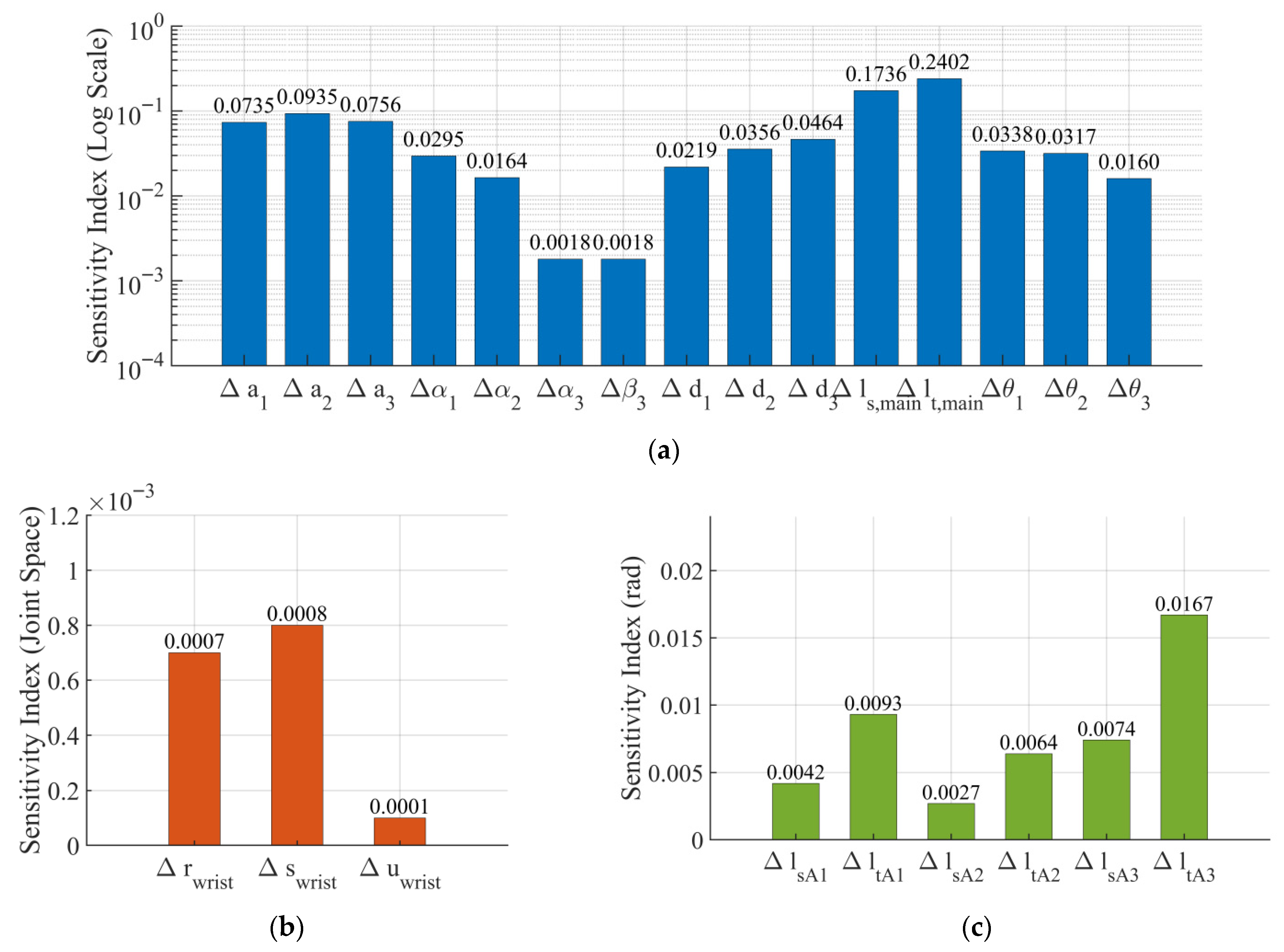
Figure 4 shows the results of the parameter sensitivity analysis within each subsystem. For the 3-DOF serial main arm (Figure 4a), the analysis clearly reveals that the transmission errors introduced by the main arm’s parallelogram mechanism are absolutely dominant. Among these, the sensitivity of the transmission-side error, Δ l t , m a i n (sensitivity: 0.2402), and the driving-side error, Δ l s , m a i n (sensitivity: 0.1736), significantly exceeds that of the standard D-H parameters. This verifies that the transmission mechanism exhibits a significant error amplification effect when operating near singular poses. Among the D-H parameters, the link length errors Δ a 1 , Δ a 2 , Δ a 3 have a secondary impact, while the influence of Δ α 3 and Δ β 3 , which are closely related to the end-effector orientation, is the least negligible. For the wrist’s transmission chain (Figure 4b), the analysis shows that the influence of the transmission-side error, Δ l t , on the output angle is generally greater than that of the driving-side error, Δ l s . At the same time, the error’s influence shows a progressive amplification trend, with the error parameter of the third-stage transmission chain, Δ l t A 3 (sensitivity: 0.0167), being the most sensitive for the 2-DOF parallel wrist (Figure 4c).
Although there are only a few geometric parameters, the analysis indicates that the importance of the platform radius errors, Δ r w r i s t (sensitivity: 0.0007) and Δ s w r i s t (sensitivity: 0.0008), is significantly higher than that of the leg length error, Δ u w r i s t (sensitivity: 0.0001). Through this hierarchical analysis, we can systematically select a reduced parameter set consisting of the 19 most sensitive parameters from the total of 24 potential error parameters (excluding Δ α 3 , Δ β 3 , Δ l s A 2 , Δ l s A 1 , Δ u w r i s t ) . This parameter set will be used for the global identification and calibration in Section 4. This approach significantly improves the computational efficiency and numerical stability of the calibration process while ensuring the completeness of the model.

4. Hierarchical Identification and Calibration

Based on the decoupled, hierarchical error model established previously, this section proposes a hierarchical calibration strategy. The core of this strategy is to independently calibrate the pose error of the 3-DOF serial main arm and the orientation error of the 2-DOF parallel wrist by utilizing different measurement devices, corresponding error models, and identification algorithms. This approach decomposes the complex, multi-parameter, coupled identification problem into two relatively independent sub-problems to improve calibration efficiency and accuracy. For the 3-DOF serial main arm, its end-effector position error stems primarily from a combination of its link geometric parameter errors and the geometric parameter errors of its parallelogram mechanism. We will employ an NDI optical measurement system to perform position measurements of the 3-DOF serial main arm and then identify the errors using the GA (Genetic Algorithm). Subsequently, for the 2-DOF parallel wrist, orientation errors are attributed to the geometric inaccuracies of the parallel mechanism itself and the accumulated errors propagated through the multi-stage transmission chain. All relevant error parameters for the wrist and its transmission chain are identified by fusing data from an attitude sensor and motor encoders. To systematically demonstrate the superiority of the proposed models and identification algorithm (GA), this section will also define a set of baseline comparison models and ablation study protocols for the calibration of the series arm and the parallel wrist, respectively. The detailed performance comparison results will be discussed in Section 6.

4.1. Pose Calibration of the 3-DOF Serial Main Arm

For the position measurement in the calibration experiment, this paper uses a Polaris Vega VT optical measurement system from NDI (Northern Digital Inc., Waterloo, ON, Canada) for high-precision pose measurement. At an operating distance of less than 3 m, this optical positioning system has an absolute distance error of up to ±60 μm, which meets the requirements of the calibration experiment. The calibration procedure is as follows: First, a series of measurement points is planned within the main arm’s workspace. Then, the manipulator is driven to reach each point sequentially, and two sets of data are recorded synchronously: the joint angles, q k , fed back by the three motor encoders of the manipulator, and the actual pose of the end-effector’s marker plate, T m , k , recorded by the NDI system.
This paper employs the GA for error parameter identification. As a global optimization algorithm, the GA can effectively handle problems with highly nonlinear models [45] and mitigates the risk of entrapment in local optima. Its fitness function is defined as the composite pose error between the theoretical pose, calculated by the error model, and the actual pose, measured by the optical measurement system, evaluated over N measurement points. The objective of the identification is to determine an optimal set of error parameters, e o p t , that minimizes the value of this fitness function. The fitness function, F(e), is expressed as:
F e = 1 N k = 1 N w p p c q k , e p m , k 2 + w o θ e r r R c q k , e , R m , k 2
where p c and p m denote the calculated and measured position vectors, respectively; R c and R m are the calculated and measured rotation matrices; θ e r r is the orientation error angle; and w p , w o are the weighting coefficients. GA optimization commences with an initial population randomly generated within the tolerance domain of the error parameters (refer to Table 2). In each generation, the fitness of every individual (i.e., a set of error parameters) within the population is evaluated according to the predefined objective function, which then determines the individual’s survival probability for producing the subsequent generation through genetic operators such as selection, crossover, and mutation. The iterative process continues until the maximum number of generations is reached or the fitness value converges, at which point the optimization terminates. The individual with the best fitness at termination represents the identified set of optimal error parameters, e o p t .

Baseline Comparison and Ablation Study (Serial Arm)

To validate the necessity of the proposed composite model, which includes the four-bar linkage transmission error (hereafter referred to as ‘Proposed—GA15’, with 15 error parameters), we designed the following baseline comparison models:
MDH-Only Model (GA13): This is an ablation study model that disregards the four-bar linkage transmission error. This model uses only standard MDH error parameters (13 parameters in total) and is also identified using GA. Comparing the results of GA15 and GA13 allows us to quantify the contribution of the four-bar linkage transmission error model to accuracy.
Deterministic Algorithm Comparison (LM15): To compare the performance of the GA global optimization algorithm, we also used the classic Levenberg–Marquardt (LM) deterministic algorithm to identify the complete 15-parameter model (Proposed).

4.2. Calibration of the 2-DOF Parallel Wrist and Its Transmission Chain

Given that the forward kinematics of the 2-DOF parallel wrist lacks a closed-form analytical solution and the remote multi-stage drive introduces nonlinear transmission errors, traditional calibration methods based on end-effector pose are rendered inapplicable. To address this challenge, this paper adopts a joint-space error calibration strategy based on the inverse kinematic model. The core of this strategy lies in using the inverse kinematic model of the parallel mechanism and the forward transmission error model of the chain to calculate two theoretical angles: the theoretical actuated output angle of the 2-DOF parallel wrist (derived from the measured moving platform orientation) and the output angle of the multi-stage transmission chain (derived from the measured motor drive angle). By minimizing the discrepancy between these two theoretical values, the geometric errors of both the parallel mechanism and the transmission chain are identified simultaneously. By effectively addressing the coupling problem between transmission and geometric errors, this approach enhances calibration efficiency and accuracy.
The objective of this calibration step is to identify the geometric errors of the entire parallel wrist system. This not only includes the parameters of the 2-DOF parallel mechanism itself ( s , r ,   u ) but also covers the parameters of the two three-stage parallelogram transmission chains ( l s A 1 , l t A 1 , l s B 1 , ,   l t B 2 ), totaling 19 parameters.
For the 2-DOF parallel calibration experiment, a high-precision WIT attitude sensor is installed on the terminal moving platform (the F 1 S 1 S 2 plane in Figure 3) to directly measure the orientation angles, γ and β, of the moving platform about the x- and y-axes. The drive motors move the parallel wrist to a series of calibration points within its reachable orientation workspace. The actual orientation angles measured by the WIT sensor, X m = x m 1 , x m 2 , , x m n , and the actual angles measured by the encoders of the actuated joints R1 and R2, Q m = { q m 1 , q m 2 , , q m n } , are recorded synchronously.
The GA is again used for identification. According to the calibration strategy based on inverse kinematics proposed in Section 2.2.3, the objective function is no longer the end-effector pose error, but rather the error in the actuated joint angles. Instead of linking geometric parameter errors to end-effector pose errors, this method uses the derived closed-form inverse solution to map parameter errors to driven joint angle errors. This approach effectively bypasses the difficulty of solving the forward kinematics.
The objective function, G(∆P, ∆X), is defined as follows:
G P , X = 1 N k = 1 N q c ( x m k , P n   +   P )     q o ( q m k , X ) 2
where
  • Δ P is the vector of error parameters to be identified for the parallel mechanism ( Δ s , Δ r , Δ u ).
  • Δ X is the vector of error parameters to be identified for the two transmission paths ( Δ l s A 1 , Δ l t A 1 , Δ l s B 1 , …).
  • x m k is the actual orientation angle ( γ k , β k ) of the k -th point measured by the WIT sensor.
  • q m k is the actually measured angle of the actuated joints R1 and R2 corresponding to the k -th orientation point.
  • q c x m k , P n + Δ P is the theoretical input angle of the parallel mechanism, calculated using the inverse kinematic error model from Equation (35), by substituting the measured orientation x m k and the geometric parameters including errors, P n + Δ P .
  • q o q m k , Δ X is the theoretical output angle from the transmission chain, calculated using its error model by substituting the measured input angle q m k and its error parameters Δ X .
The subsequent identification process is similar to that in Section 4.1. By leveraging the global search capability of the GA, an optimal set of error parameters, Δ P o p t and Δ X o p t , is sought in the multi-dimensional parameter space to minimize the objective function for the joint-space error, G Δ P , Δ X . Through the hierarchical identification and calibration method described above, the key geometric error parameters of each part of the manipulator can be obtained efficiently and accurately, laying the foundation for subsequent error compensation and accuracy enhancement.

Baseline Comparison and Ablation Study (Parallel Wrist)

To validate the effectiveness of the proposed physics-based identification strategy for the multi-stage transmission chain of the parallel wrist (hereafter referred to as ‘Proposed—GA’), we designed the following comparative models:
2nd-Order Polynomial Fit Model (2nd-Poly—GA): This model uses the inverse kinematic model but replaces the complex physical transmission chain model. It assumes the transmission error (the difference between the theoretical output angle and the motor input angle) can be fitted by a second-order polynomial: Δ q = c 2 q i n 2 + c 1 q i n + c 0 . The identification process (GA) simultaneously identifies the geometric parameters of the parallel wrist and the polynomial coefficients.
1st-Order Polynomial Fit Model (1st-Poly—GA): Similar to the model above but uses a first-order polynomial Δ q = c 1 q i n + c 0 for fitting.
Zero-Calibration Model (Zero-Cal—GA): This is the most simplified baseline, assuming all errors manifest as zero-offset biases in the drive joints, i.e., only identifying the Δ q 1 , Δ q 2 zero-offset error parameters.
All comparative models are identified using GA and evaluated on the same validation dataset.

5. Calibration Experiment

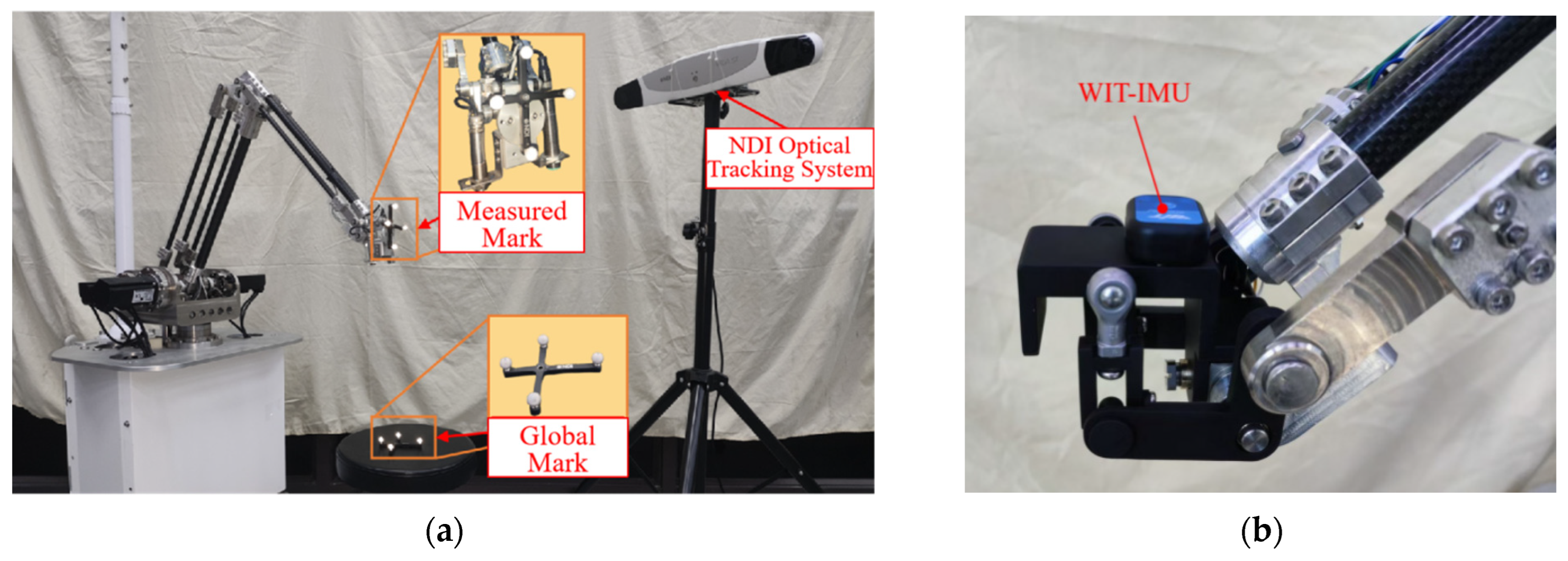
To validate the effectiveness of the aforementioned layered identification and calibration method, we constructed an experimental calibration system based on a self-developed 5-DOF hybrid manipulator prototype (as shown in Figure 5). The core equipment includes an NDI Polaris Vega VT optical measurement system (accuracy: ±60 µm) for 3D position tracking and a high-precision WIT attitude sensor (accuracy: ±0.1°) for orientation measurement.
The experimental setup is as follows. For the 3-DOF main arm calibration (Figure 5a), a target plate equipped with four non-collinear optical markers was mounted on the end of the serial main arm. Additionally, a static reference marker was positioned near the robot base to establish a global coordinate frame. For the 2-DOF wrist calibration (Figure 5b), the high-precision WIT attitude sensor was rigidly mounted to the end-effector’s moving platform. This sensor directly measured the platform’s orientation angles, γ and β, around the x- and y-axes, respectively, while the input angles of the transmission chain were recorded by encoders.
Prior to calibration, coordinate registration is performed using discrete feature points. Theoretical coordinates, P B , of at least three non-collinear markers in the robot base frame, O B , are obtained from the design model. Corresponding markers are rigidly mounted on the experimental setup, and their actual coordinates, P c , are captured by the NDI system in the measurement frame, O C . By solving the Absolute Orientation Problem (AOP) [46] to minimize the root-mean-square error (RMSE) between these point sets, the homogeneous transformation matrix, T, is calculated. This matrix unifies all subsequent measurements into the base frame, eliminating systematic errors caused by arbitrary sensor placement.
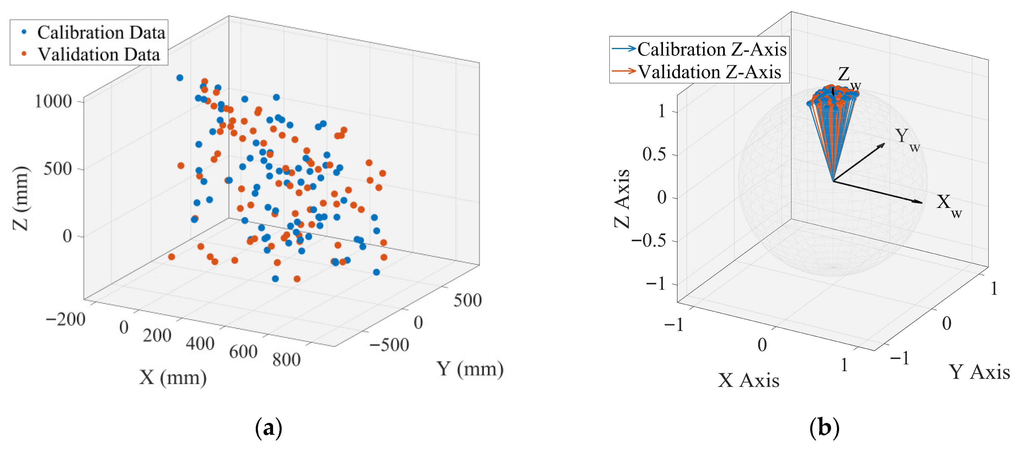
The data collection procedure comprises two stages. The first stage addresses the pose accuracy of the 3-DOF serial main arm. A target plate with optical markers was attached to the end-effector. As shown in Figure 6a, 160 measurement points were planned within the workspace, split equally into calibration (80) and validation (80) sets to evaluate model generalization and prevent overfitting. The manipulator sequentially traversed these points while the NDI system recorded the spatial pose errors, forming the serial arm dataset P_m. The second stage focuses on the orientation accuracy of the 2-DOF parallel wrist. As depicted in Figure 6b, 60 calibration and 60 validation poses were collected. At each pose, the platform orientation angles γ m , β m from the WIT sensor and the transmission input angles q m 1 , q m 2 from motor encoders were synchronously recorded. Additionally, to assess robustness, a “stress test” dataset comprising 30 points near transmission singularities was collected. This dataset serves to evaluate model performance under worst-case conditions.

6. Results and Discussion

This section presents the experimental results based on the hierarchical calibration strategy and dataset protocols defined in Section 4 and Section 5. The identified kinematic parameters are presented in Table 3. We first analyze the results for the 3-DOF serial arm, including baseline comparisons, robustness stress tests, and algorithm stability. We then present the results for the 2-DOF parallel wrist, including its ablation studies.

6.1. Serial Arm Calibration Results and Ablation Study

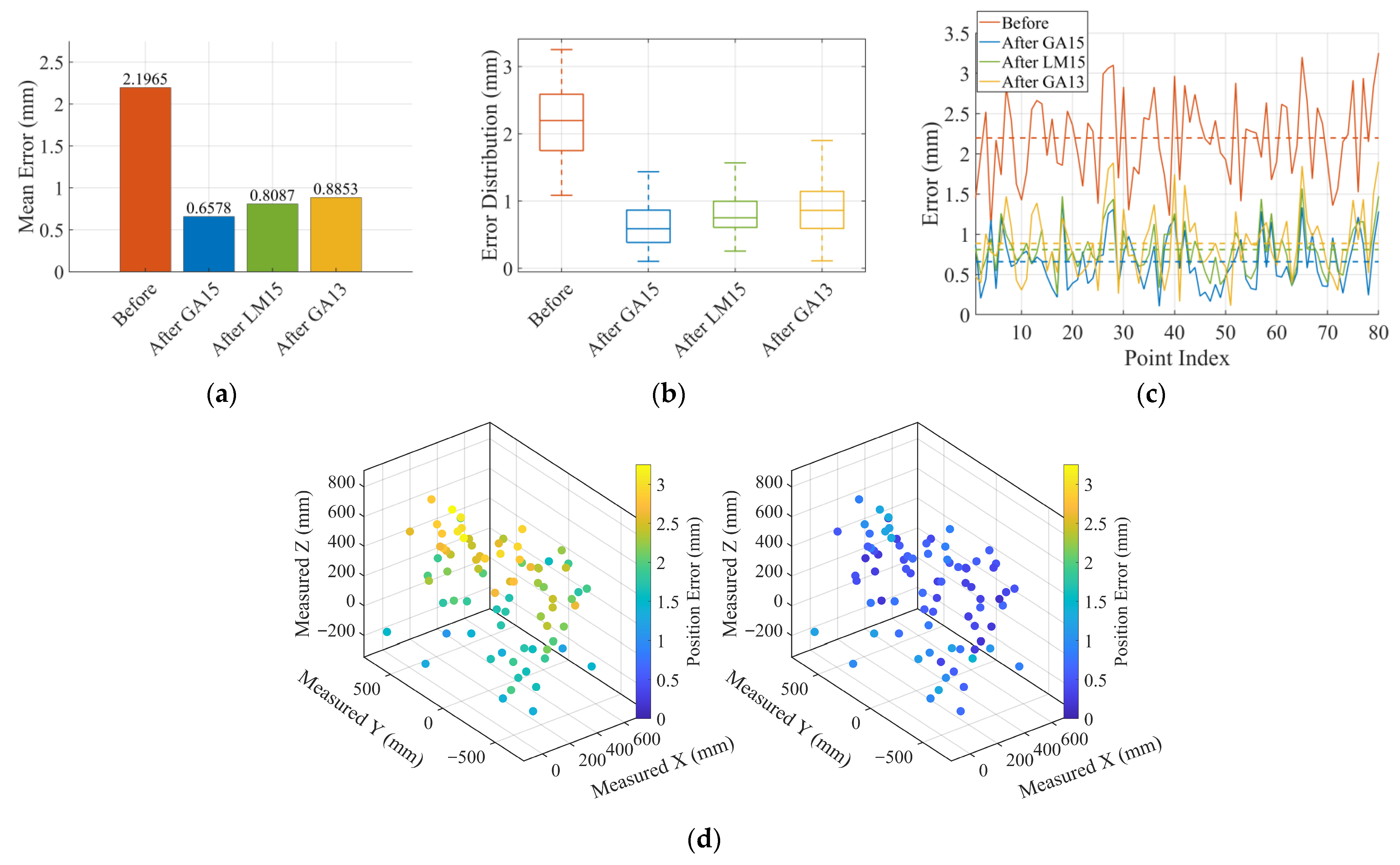
First, the 3-DOF serial arm was calibrated. The results of the proposed method versus the baseline models, all evaluated on the 80-point independent validation dataset, are shown in Figure 7. As shown in Figure 7a, the mean position error of the manipulator before calibration was substantial, measuring 2.199 mm. Employing the proposed GA15 model (incorporating both MDH and four-bar linkage transmission errors), the mean error was reduced to 0.658 mm. This corresponds to a 70.1% accuracy improvement, validating the method’s effectiveness.
We then evaluated the baseline models defined in Section Baseline Comparison and Ablation Study (Serial Arm):
Algorithm Comparison: The LM15 method (using the deterministic LM algorithm on the same 15-parameter model) reduced the mean error to 0.809 mm. While effective, it underperformed compared to the GA15 method (0.658 mm). This suggests that for this complex, nonlinear model, the global search capability of the GA successfully avoided local optima that likely trapped the LM algorithm, thus finding a superior parameter solution. Ablation Study: Most importantly, the MDH-Only (GA13) model, which removed the four-bar linkage transmission error model, could only reduce the mean error to 0.885 mm. This forcefully demonstrates that the nonlinear error introduced by the four-bar linkage transmission mechanism is a dominant error source. The proposed composite error model is therefore essential and critical for accurately calibrating this class of manipulator. Figure 7b further confirms this with a box plot of the error distributions. The Proposed—GA15 method not only has the lowest median error but also the narrowest interquartile range, indicating a more stable and robust calibration result. Figure 7c shows the point-by-point error, where the Proposed—GA15 outperforms the other methods at the vast majority of validation points. Finally, Figure 7d provides a spatial error map. Before calibration, large errors (>3 mm) were concentrated in regions with high z-axis and large x-axis values. After calibration, the errors at all points are significantly reduced and distributed much more uniformly across the workspace, visually demonstrating the calibration’s global effectiveness.
Additionally, as the GA is a stochastic optimization algorithm, its stability and repeatability were evaluated. We conducted 20 independent calibration runs on the serial arm’s Proposed-GA15 model, each initialized with a distinct random seed. The results showed high consistency: the post-calibration mean RMSE across all 20 runs was 0.5722 mm with a standard deviation of only 0.0071 mm. This demonstrates that the GA exhibits high repeatability and reliably converges to a high-quality solution.

6.2. Serial Arm Robustness in Singular Region (Stress Test)

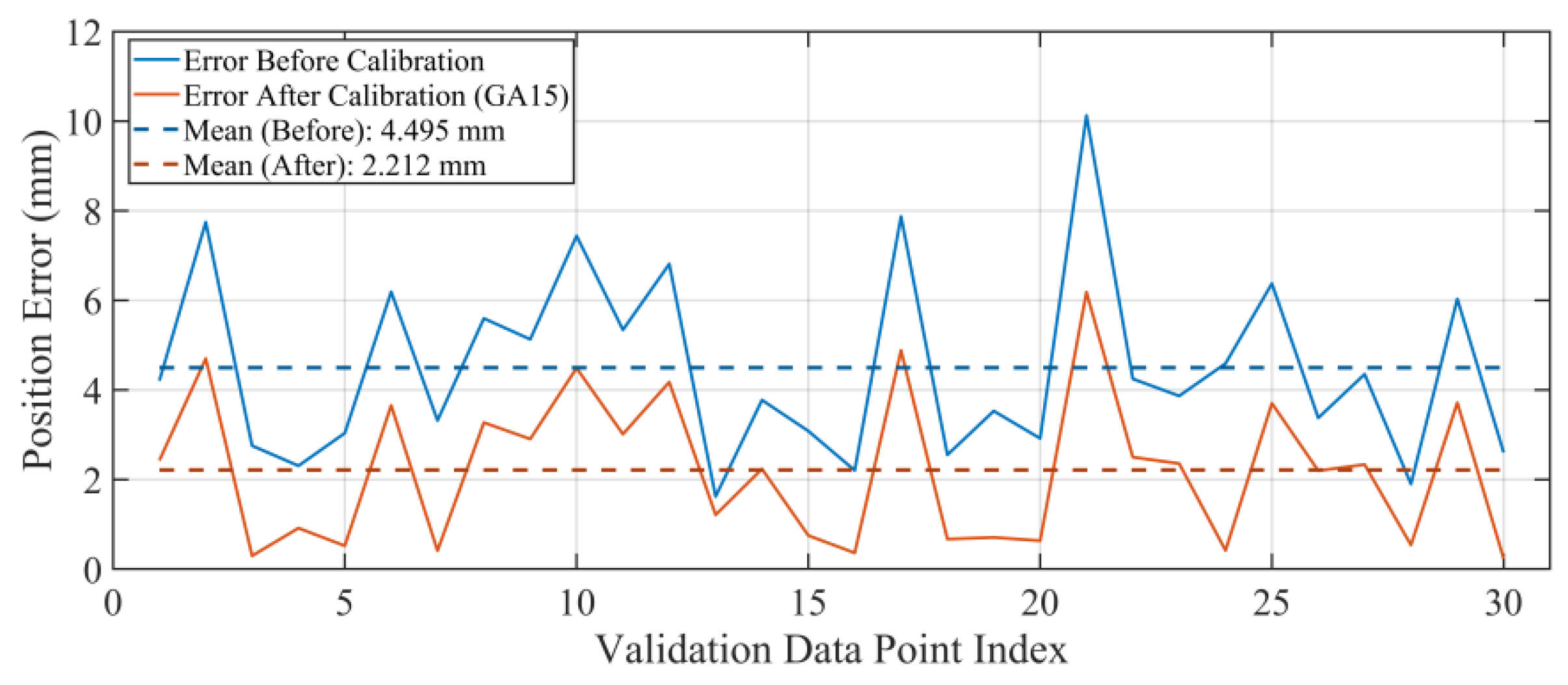
To evaluate the robustness of the identification algorithm, specific ‘stress test’ datasets were collected in regions close to the mechanism’s transmission singularities. Mathematically, these singular configurations were identified by analyzing the kinematic Jacobian matrix ( J ) of the transmission chain 1. A singularity occurs when the determinant of the Jacobian matrix approaches zero ( d e t ( J ) 0 ), leading to a loss of rank [47]. For the parallelogram mechanism utilized in this study (modeled in Equation (7)), these singularities correspond to the driving angle φ 2 approaching 0 or π. Operating near singular configurations leads to a sharp increase in actuation forces and error sensitivity, which is often referred to as ‘closeness to singularity’ [48]. To test the algorithm’s robustness in these sensitive regions, we defined the singular test region as the configuration space where the transmission angle deviates from the critical limit by less than 5°. In these regions, the error amplification factor increases significantly, making the system highly sensitive to geometric parameters and providing a rigorous testbed for the algorithm’s stability.
The results are shown in Figure 8. On this dataset, the pre-calibration mean position error was as high as 4.495 mm due to the proximity to the singularity. After calibration with our model, the mean error was still significantly reduced to 2.212 mm, a 50.8% improvement. Although the residual error of 2.212 mm is higher than that on the standard validation set (0.658 mm), positions near singularities can be avoided in practice by restricting joint angles via software limits. Meanwhile, this experiment demonstrates that the proposed model still significantly improves positioning accuracy, even when operating near these singular positions.

6.3. Parallel Wrist Calibration Results and Ablation Study

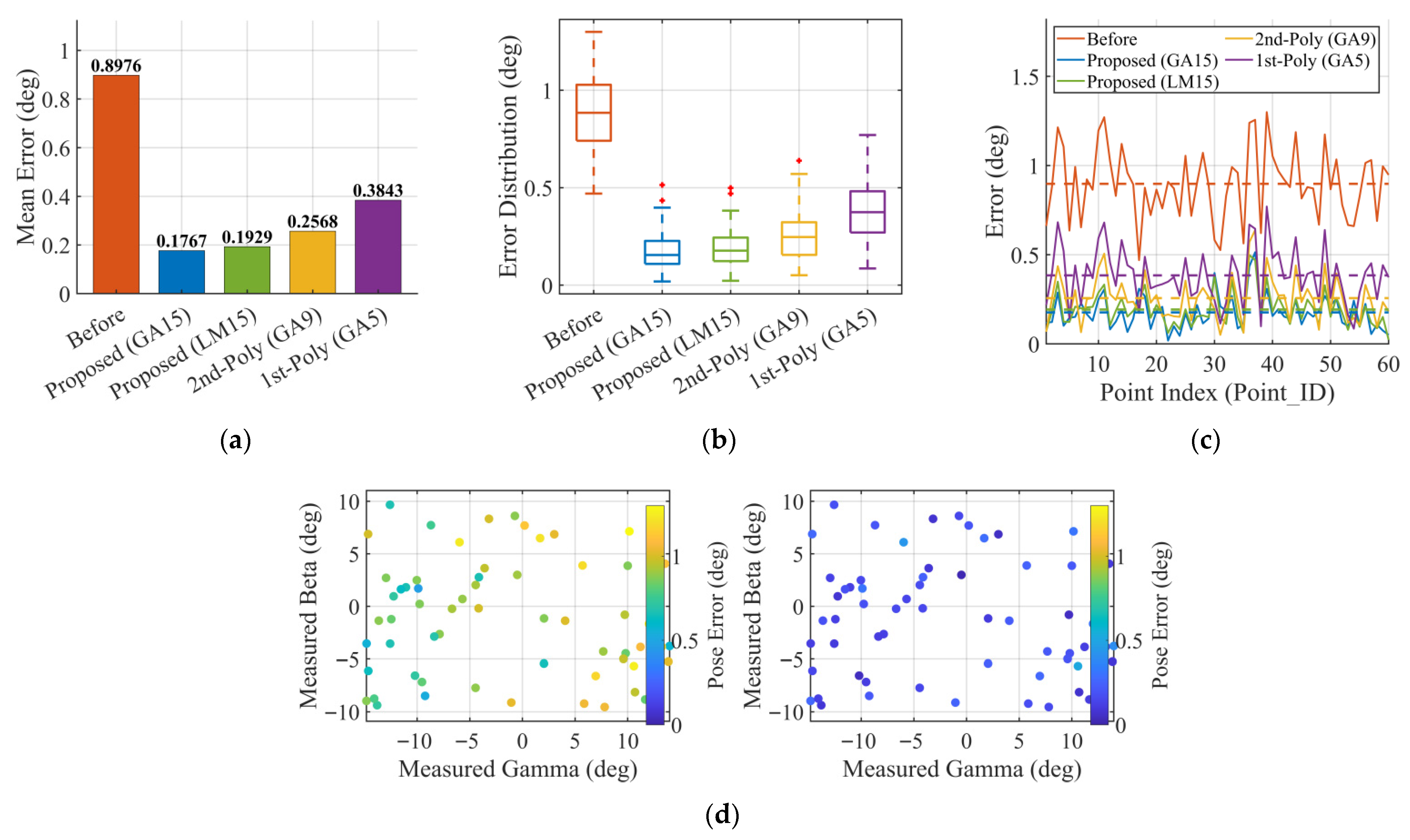
Next, the 2-DOF parallel wrist and its transmission chains were calibrated. Figure 9 shows the results of its comparative experiments. As shown in Figure 9a, the mean orientation error of the parallel wrist before calibration was 0.8976 deg. Using the physics-based model proposed in this paper, the Proposed-GA method reduced the mean error to 0.1767 deg. In contrast, the mean error using the LM algorithm was 0.1929 deg. The superior result of GA over LM demonstrates its global optimization advantage in handling such complex nonlinear models. To verify the necessity of the physics-based model, we compared it with simplified models. The 2nd-Poly (GA9) model’s mean error was 0.2568 deg, and the 1st-Poly model’s mean error was 0.3843 deg. In conclusion, the calibration effect of the proposed physics-based transmission error model is significantly superior to methods using generic polynomial fitting, and also surpasses the identification results of the LM algorithm. This validates the accuracy and necessity of the multi-stage transmission chain model established in this paper, confirming that simple fitting functions are insufficient to capture the complex nonlinear error characteristics inherent to the system [49,50]. Finally, the spatial error map in Figure 9d visualizes the post-calibration residuals, demonstrating the method’s efficacy across the entire orientation workspace.

7. Conclusions and Future Work

This paper proposes and validates an innovative hierarchical and decoupled high-precision calibration framework for a class of serial-parallel hybrid robots featuring parallelogram mechanisms for remote actuation. The framework offers two core contributions: first, it accurately quantifies the coupled errors of the 3-DOF serial main arm and its transmission chain through a composite error model; second, it employs a joint-space error identification strategy based on inverse kinematics, which circumvents the intractability of solving the forward kinematics for the 2-DOF parallel wrist.
The experimental results confirmed the framework’s effectiveness. Crucially, through comprehensive baseline comparisons and ablation studies, this paper quantitatively demonstrates that the proposed composite error model, based on the transmission chain model, is essential for achieving high accuracy, with its performance significantly surpassing standard or simplified calibration methods.
Despite the effective results, this study has several limitations. The models established herein focus primarily on kinematic errors and do not yet account for nonlinear dynamic effects, such as elastic deformation under load, joint backlash, or friction. Consequently, the calibration was performed under quasi-static conditions.
Future work will primarily address these limitations. First, dynamic calibration will be investigated, establishing a more comprehensive error model to compensate for errors induced by speed, inertia, and varying loads. Second, the integration of machine learning methods with the physics-based model will be explored to compensate for residual nonlinear errors not captured by the current model. Finally, based on the high-precision model, hybrid force/position control under redundant actuation [51], will be studied to achieve high-precision dynamic control of the manipulator in precision industrial scenarios.

Author Contributions

Conceptualization, Z.W., H.Y. and J.Z.; methodology, Z.W. and Y.C.; software, Z.W.; validation, X.W. and Y.M.; formal analysis, Z.W.; investigation, Y.C.; resources, X.W.; data curation, Z.W.; writing—original draft preparation, Z.W.; writing—review and editing, Z.W. and H.Y.; visualization, Y.W.; supervision, H.Y.; project administration, J.Z.; funding acquisition, J.Z. All authors have read and agreed to the published version of the manuscript.

Funding

This research was funded by the National Key R&D Program of China, grant number 2019YFC1711800, the Key R&D Program of Jiangsu Science and Technology Project, grant number BE2021661, the Key R&D Program of Jiangsu Science and Technology Project (grant number BE2022049), the Suzhou Science and Technology Project, grant number SLJ2021021, the Project of Jiangsu Province High-End Medical Devices Technology Innovation Center, grant number LHYF20240202.

Data Availability Statement

The data presented in this study are available on request from the corresponding author.

Conflicts of Interest

The authors declare no conflicts of interest.

References

  1. Zhang, Y.L.; Guan, E.G.; Li, P.B.; Zhao, Y.Z. An automated nondestructive testing system for the surface of pressure pipeline welds. J. Field Robot. 2023, 40, 1927–1944. [Google Scholar] [CrossRef]
  2. Cheng, Y.S.; Yen, S.H.; Bedaka, A.K.; Shah, S.H.; Lin, C.Y. Trajectory planning method with grinding compensation strategy for robotic propeller blade sharpening application. J. Manuf. Process. 2023, 86, 294–310. [Google Scholar] [CrossRef]
  3. Wu, Z.H.; Wang, X.L.; Lyu, Z.K.; Xu, Q.S. Design of a Novel Passive Polishing End-Effector with Adjustable Constant Force and Wide Operating Angle. IEEE-ASME Trans. Mechatron. 2024, 29, 4330–4340. [Google Scholar] [CrossRef]
  4. Xie, J.C.; Liu, Y.L.; Wang, X.W.; Fang, S.K.; Liu, S.G. A new XR-based human-robot collaboration assembly system based on industrial metaverse. J. Manuf. Syst. 2024, 74, 949–964. [Google Scholar] [CrossRef]
  5. Huang, Z.; Li, Q.C. General methodology for type synthesis of symmetrical lower-mobility parallel manipulators and several novel manipulators. Int. J. Robot. Res. 2002, 21, 131–145. [Google Scholar] [CrossRef]
  6. Merlet, J.-P. Parallel Robots; Springer: Berlin/Heidelberg, Germany, 2006. [Google Scholar]
  7. Wang, J.; Wu, C.; Liu, X.-J. Performance evaluation of parallel manipulators: Motion/force transmissibility and its index. Mech. Mach. Theory 2010, 45, 1462–1476. [Google Scholar] [CrossRef]
  8. Khalid, A.; Mekid, S. Intelligent spherical joints based tri-actuated spatial parallel manipulator for precision applications. Robot. Comput.-Integr. Manuf. 2018, 54, 173–184. [Google Scholar] [CrossRef]
  9. Cheng, G.; Xu, P.; Yang, D.H.; Liu, H.G. Stiffness analysis of a 3CPS parallel manipulator for mirror active adjusting platform in segmented telescope. Robot. Comput.-Integr. Manuf. 2013, 29, 302–311. [Google Scholar] [CrossRef]
  10. Zhang, N.B.; Huang, P.C.; Li, Q.C. Modeling, design and experiment of a remote-center-of-motion parallel manipulator for needle insertion. Robot. Comput.-Integr. Manuf. 2018, 50, 193–202. [Google Scholar] [CrossRef]
  11. Lee, M.K.; Park, K.W.; Choi, B.O. Kinematic and dynamic models of hybrid robot manipulator for propeller grinding. J. Robot. Syst. 1999, 16, 137–150. [Google Scholar] [CrossRef]
  12. Antonov, A.; Fomin, A.; Glazunov, V.; Kiselev, S.; Carbone, G. Inverse and forward kinematics and workspace analysis of a novel 5-DOF (3T2R) parallel-serial (hybrid) manipulator. Int. J. Adv. Robot. Syst. 2021, 18, 14. [Google Scholar] [CrossRef]
  13. Xu, P.; Cheung, C.F.; Li, B.; Ho, L.T.; Zhang, J.F. Kinematics analysis of a hybrid manipulator for computer controlled ultra-precision freeform polishing. Robot. Comput.-Integr. Manuf. 2017, 44, 44–56. [Google Scholar] [CrossRef]
  14. Zhou, M.C.; Yu, Q.M.; Huang, K.; Mahov, S.; Eslami, A.; Maier, M.; Lohmann, C.P.; Navab, N.; Zapp, D.; Knoll, A.; et al. Towards Robotic-Assisted Subretinal Injection: A Hybrid Parallel-Serial Robot System Design and Preliminary Evaluation. IEEE Trans. Ind. Electron. 2020, 67, 6617–6628. [Google Scholar] [CrossRef]
  15. Lai, Y.L.; Liao, C.C.; Chao, Z.G. Inverse kinematics for a novel hybrid parallel serial five-axis machine tool. Robot. Comput.-Integr. Manuf. 2018, 50, 63–79. [Google Scholar] [CrossRef]
  16. Laryushkin, P.; Antonov, A.; Fomin, A.; Essomba, T. Velocity and Singularity Analysis of a 5-DOF (3T2R) Parallel-Serial (Hybrid) Manipulator. Machines 2022, 10, 276. [Google Scholar] [CrossRef]
  17. Antonov, A.; Fomin, A.; Glazunov, V.; Petelin, D.; Filippov, G. Type Synthesis of 5-DOF Hybrid (Parallel-Serial) Manipulators Designed from Open Kinematic Chains. Robotics 2023, 12, 98. [Google Scholar] [CrossRef]
  18. Gallardo-Alvarado, J. Kinematics of a hybrid manipulator by means of screw theory. Multibody Syst. Dyn. 2005, 14, 345–366. [Google Scholar] [CrossRef]
  19. Lu, Y.; Hu, B. Solving driving forces of 2(3-SPR) serial-parallel manipulator by CAD variation geometry approach. J. Mech. Des. 2006, 128, 1349–1351. [Google Scholar] [CrossRef]
  20. Hu, B.; Yu, J.J. Unified solving inverse dynamics of 6-DOF serial-parallel manipulators. Appl. Math. Model. 2015, 39, 4715–4732. [Google Scholar] [CrossRef]
  21. Boby, R.A.; Klimchik, A. Combination of geometric and parametric approaches for kinematic identification of an industrial robot. Robot. Comput.-Integr. Manuf. 2021, 71, 14. [Google Scholar] [CrossRef]
  22. Shen, H.P.; Meng, Q.M.; Li, J.; Deng, J.M.; Wu, G.L. Kinematic sensitivity, parameter identification and calibration of a non-fully symmetric parallel Delta robot. Mech. Mach. Theory 2021, 161, 20. [Google Scholar] [CrossRef]
  23. Camacho-Arreguin, J.; Wang, M.F.; Dong, X.; Axinte, D. A novel class of reconfigurable parallel kinematic manipulators: Concepts and Fourier-based singularity analysis. Mech. Mach. Theory 2020, 153, 16. [Google Scholar] [CrossRef]
  24. Carbonari, L.; Callegari, M.; Palmieri, G.; Palpacelli, M.C. Analysis of Kinematics and Reconfigurability of a Spherical Parallel Manipulator. IEEE Trans. Robot. 2014, 30, 1541–1547. [Google Scholar] [CrossRef]
  25. Carbonari, L.; Callegari, M.; Palmieri, G.; Palpacelli, M.C. A new class of reconfigurable parallel kinematic machines. Mech. Mach. Theory 2014, 79, 173–183. [Google Scholar] [CrossRef]
  26. Zhao, Y.Q.; Jin, Y.; Anderson, H.; Higgins, C. A new reconfigurable parallel mechanism using novel lockable joints for large scale manufacturing. Robot. Comput.-Integr. Manuf. 2023, 82, 11. [Google Scholar] [CrossRef]
  27. Roth, Z.S.; Mooring, B.W.; Ravani, B. An overview of robot calibration. IEEE J. Robot. Autom. 1987, 3, 377–385. [Google Scholar] [CrossRef]
  28. Jiang, Z.H.; Zhou, W.G.; Li, H.; Mo, Y.; Ni, W.C.; Huang, Q. A New Kind of Accurate Calibration Method for Robotic Kinematic Parameters Based on the Extended Kalman and Particle Filter Algorithm. IEEE Trans. Ind. Electron. 2018, 65, 3337–3345. [Google Scholar] [CrossRef]
  29. Wu, Y.; Klimchik, A.; Caro, S.; Furet, B.; Pashkevich, A. Geometric calibration of industrial robots using enhanced partial pose measurements and design of experiments. Robot. Comput.-Integr. Manuf. 2015, 35, 151–168. [Google Scholar] [CrossRef]
  30. Sun, T.; Zhai, Y.P.; Song, Y.M.; Zhang, J.T. Kinematic calibration of a 3-DoF rotational parallel manipulator using laser tracker. Robot. Comput.-Integr. Manuf. 2016, 41, 78–91. [Google Scholar] [CrossRef]
  31. Luo, G.Y.; Zou, L.; Wang, Z.L.; Lv, C.; Ou, J.; Huang, Y. A novel kinematic parameters calibration method for industrial robot based on Levenberg-Marquardt and Differential Evolution hybrid algorithm. Robot. Comput.-Integr. Manuf. 2021, 71, 11. [Google Scholar] [CrossRef]
  32. Denavit, J.; Hartenberg, R.S. A kinematic notation for lower-pair mechanisms based on matrices. J. Appl. Mech. 1955, 22, 215–221. [Google Scholar] [CrossRef]
  33. Hayati, S.; Mirmirani, M. Improving the absolute positioning accuracy of robot manipulators. J. Robot. Syst. 1985, 2, 397–413. [Google Scholar] [CrossRef]
  34. Zhuang, H.; Roth, Z.S.; Hamano, F. A complete and parametrically continuous kinematic model for robot manipulators. IEEE Trans. Robot. Autom. 1992, 8, 451–463. [Google Scholar] [CrossRef]
  35. Wu, L.; Yang, X.D.; Chen, K.; Ren, H.L. A Minimal POE-Based Model for Robotic Kinematic Calibration with Only Position Measurements. IEEE Trans. Autom. Sci. Eng. 2015, 12, 758–763. [Google Scholar] [CrossRef]
  36. Tian, W.J.; Mou, M.W.; Yang, J.H.; Yin, F.W. Kinematic calibration of a 5-DOF hybrid kinematic machine tool by considering the ill-posed identification problem using regularisation method. Robot. Comput.-Integr. Manuf. 2019, 60, 49–62. [Google Scholar] [CrossRef]
  37. Sun, T.; Lian, B.B.; Yang, S.F.; Song, Y.M. Kinematic Calibration of Serial and Parallel Robots Based on Finite and Instantaneous Screw Theory. IEEE Trans. Robot. 2020, 36, 816–834. [Google Scholar] [CrossRef]
  38. He, J.; Ding, Q.Y.; Gao, F.; Zhang, H.B. Kinematic calibration methodology of hybrid manipulator containing parallel topology with main limb. Measurement 2020, 152, 11. [Google Scholar] [CrossRef]
  39. Codourey, A. Dynamic modelling and mass matrix evaluation of the DELTA parallel robot for axes decoupling control. In Proceedings of the 1996 IEEE/RSJ International Conference on Intelligent Robots and Systems—Robotic Intelligence Interacting with Dynamic Worlds (IROS 96), Senri Life Sci Ctr, Osaka, Japan, 4–8 November 1996; pp. 1211–1218. [Google Scholar]
  40. Ni, Y.B.; Jia, S.L.; Zhang, Z.W.; Wang, J.X.; Liu, X.; Li, J.H. A manufacturing-oriented error modelling method for a hybrid machine tool based on the 3-PRS parallel spindle head. Adv. Mech. Eng. 2019, 11, 13. [Google Scholar] [CrossRef]
  41. Liu, H.T.; Huang, T.; Chetwynd, D.G. A General Approach for Geometric Error Modeling of Lower Mobility Parallel Manipulators. J. Mech. Robot. 2011, 3, 13. [Google Scholar] [CrossRef]
  42. Joubair, A.; Bonev, I.A. Comparison of the efficiency of five observability indices for robot calibration. Mech. Mach. Theory 2013, 70, 254–265. [Google Scholar] [CrossRef]
  43. Yang, X.L.; Wu, H.T.; Li, Y.; Chen, B. A dual quaternion solution to the forward kinematics of a class of six-DOF parallel robots with full or reductant actuation. Mech. Mach. Theory 2017, 107, 27–36. [Google Scholar] [CrossRef]
  44. Gan, D.M.; Dai, J.S.; Dias, J.; Seneviratne, L. Unified Kinematics and Singularity Analysis of a Metamorphic Parallel Mechanism with Bifurcated Motion. J. Mech. Robot. 2013, 5, 11. [Google Scholar] [CrossRef]
  45. Fan, C.; Zhao, G.L.; Zhao, J.; Zhang, L.; Sun, L.N. Calibration of a parallel mechanism in a serial-parallel polishing machine tool based on genetic algorithm. Int. J. Adv. Manuf. Technol. 2015, 81, 27–37. [Google Scholar] [CrossRef]
  46. Nubiola, A.; Bonev, I.A. Absolute robot calibration with a single telescoping ballbar. Precis. Eng.-J. Int. Soc. Precis. Eng. Nanotechnol. 2014, 38, 472–480. [Google Scholar] [CrossRef]
  47. Laryushkin, P.; Fomin, A.; Antonov, A. Kinematic and singularity analysis of a 4-DOF Delta-type parallel robot. J. Braz. Soc. Mech. Sci. Eng. 2023, 45, 218. [Google Scholar] [CrossRef]
  48. Laryushkin, P.; Fomin, A.; Antonov, A.; Glazunov, V. Virtual and Physical Prototyping of the 4-DOF Delta-type Parallel Robot Based on the Criteria of Closeness to Singularity. In Proceedings of the MSR-RoManSy 2024, Combined IFToMM Symposium of RoManSy and USCToMM Symposium on Mechanical Systems and Robotics, Knoxville, TN, USA, 19–22 June 2024; Springer Nature: Cham, Switzerland, 2024; pp. 167–178. [Google Scholar]
  49. Zhao, C.; Guo, H.; Liu, R.; Deng, Z.; Li, B.; Tian, J. Actuation distribution and workspace analysis of a novel 3 (3RRlS) metamorphic serial-parallel manipulator for grasping space non-cooperative targets. Mech. Mach. Theory 2019, 139, 424–442. [Google Scholar] [CrossRef]
  50. Guo, H.W.; Zhao, C.; Li, B.; Liu, R.Q.; Deng, Z.Q.; Tian, J. A Transformation Method to Generate the Workspace of an n(3RRS) Serial-Parallel Manipulator. J. Mech. Des. 2019, 141, 9. [Google Scholar] [CrossRef]
  51. Liu, H.T.; Yan, Z.B.; Xiao, J.L. Pose error prediction and real-time compensation of a 5-DOF hybrid robot. Mech. Mach. Theory 2022, 170, 19. [Google Scholar] [CrossRef]
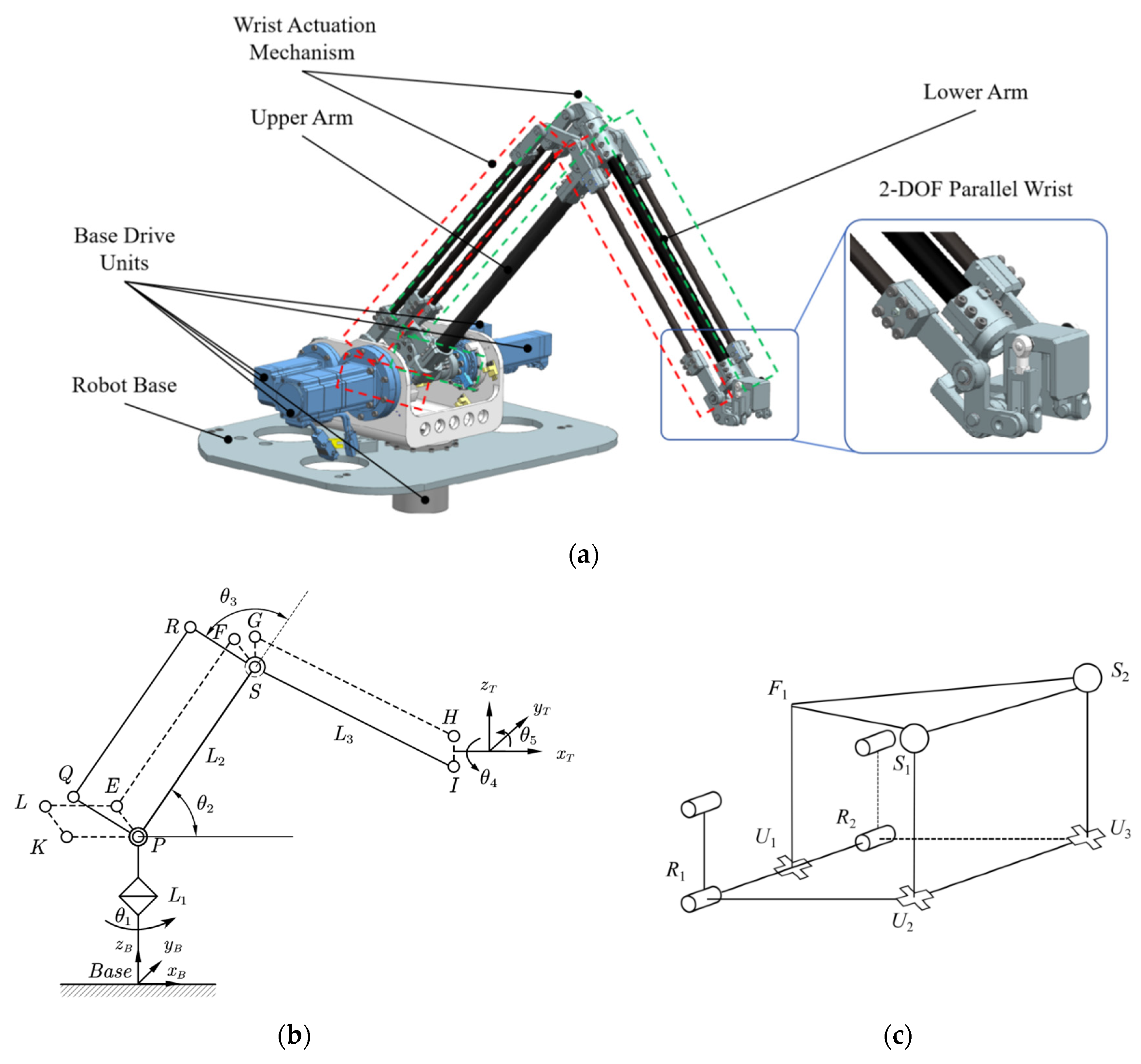
Figure 1. Error modeling for the remote drive transmission chain of the wrist mechanism: (a) Virtual prototype; (b) Overall kinematic diagram; (c) Topology of the parallel wrist.
Actuators 14 00577 g001
Figure 2. Error modeling for the remote drive transmission chain of the wrist mechanism: (a) Closed-loop vector model of the first-stage parallelogram LEPK; (b) Schematic of the multi-stage transmission chain for the wrist joint.
Actuators 14 00577 g002
Figure 3. Parallel Wrist Mechanism: (a) Virtual prototype; (b) kinematic diagram.
Actuators 14 00577 g003
Figure 4. Sensitivity Analysis of Geometric Error Parameters for Robot Subsystems: (a) Sensitivity Analysis of 3-DOF Serial Arm; (b) Sensitivity Analysis of Wrist Transmission Linkage; (c) Sensitivity Analysis of 2-DOF Wrist.
Actuators 14 00577 g004
Figure 5. Experimental setup for kinematic calibration of 5-DOF manipulator: (a) Calibration of the 3-DOF main arm; (b) Calibration of the 2-DOF wrist.
Actuators 14 00577 g005
Figure 6. (a) Position distribution for position accuracy calibration and validation; (b) Orientation distribution for pose accuracy calibration and validation.
Actuators 14 00577 g006
Figure 7. Calibration results and baseline comparison for the 3-DOF serial arm on the validation dataset. (a) Comparison of mean position errors. (b) Box plot of position error distributions. (c) Position errors for each validation point, and the dashed lines represent the mean error values of the corresponding methods. (d) Spatial comparison of position errors before and after calibration.
Actuators 14 00577 g007
Figure 8. Validation results of the GA15 model on the Stress Test Dataset.
Actuators 14 00577 g008
Figure 9. Calibration results and ablation study for the 2-DOF parallel wrist on the validation dataset. (a) Comparison of mean pose errors. (b) Box plot of pose error distributions. (c) Pose errors for each validation point, and the dashed lines represent the mean error values of the corresponding methods. (d) Spatial error map of the parallel wrist before and after calibration.
Actuators 14 00577 g009
Table 1. Nominal Kinematic Parameters of the Manipulator.
ParameterNominal ValueParameterNominal ValueParameterNominal ValueParameterNominal ValueParameterNominal Value
a 1 0 mm a 2 500 mm a 3 430 mm β 3 s40 mm
α 1 90° α 2 α 3 90°r42.5 mm l s 74 mm
d 1 80 mm d 2 0 d 3 0 mm u 49 mm l p 1 50 mm
l p 2 100 mm l p 3 74 mm l p 4 24 mm
Table 2. The tolerances and order numbers of geometric source errors in 5-DOF hybrid manipulator.
Order NumberErrorToleranceOrder NumberErrorToleranceOrder NumberErrorToleranceOrder NumberErrorTolerance
1 a 1 0.115 mm7 d 2 0.06213 β 3 0.2°19 l s A 1 0.074 mm
2 α 1 0.2°8 θ 2 0.2°14 l s 0.074 mm20 l t A 1 0.155 mm
3 d 1 0.037 mm9 a 3 0.155 mm15 l t 0.155 mm21 l s A 2 0.074 mm
4 θ 1 0.2°10 α 3 0.2°16 s 0.052 mm22 l t A 2 0.155 mm
5 a 2 0.155 mm11 d 3 0.074 mm17 r0.062 mm23 l s A 3 0.074 mm
6 α 2 0.2°12 θ 3 0.2°18 u 0.062 mm24 l t A 3 0.155 mm
Table 3. The kinematic parameter calibration results.
Serial ArmParameterIdentified
Value
ParameterIdentified ValueParameterIdentified
Value
ParameterIdentified
Value
a 1 0.209 mm α 1 0.498° d 1 0.037 mm θ 1 0.394°
a 2 −0.179 mm α 2 0.420° d 2 0.739 mm θ 2 0.420°
a 3 0.844 mm α 3 - d 3 0.074 mm θ 3 0.397°
β 3 - l s 0.0122 mm l t −0.119 mm
Parallel WristParameterIdentified
Value
ParameterIdentified ValueParameterIdentified
Value
ParameterIdentified
Value
l s A 1 - l t A 1 0.025 mm l s A 2 - l t A 2 −0.003 mm
l s A 3 0.124 mm l t A 3 0.472 mm l s B 1 −0.128 mm l t B 1 0.003 mm
l s B 2 −0.308 mm l t B 2 0.166 mm l s B 3 0.309 mm l t B 3 −0.315 mm
s −0.08 mm r0.349 mm u -
Disclaimer/Publisher’s Note: The statements, opinions and data contained in all publications are solely those of the individual author(s) and contributor(s) and not of MDPI and/or the editor(s). MDPI and/or the editor(s) disclaim responsibility for any injury to people or property resulting from any ideas, methods, instructions or products referred to in the content.