1. Introduction
Computer Numerical Control (CNC) machine tools are a key indicator of the development level of a country’s or region’s equipment manufacturing industry. They serve as essential processing equipment in aerospace, defense, automotive, electronic information, and other high-end manufacturing sectors, and have long constituted a crucial domain of national competition. The principal performance metric for CNC machine tools is machining accuracy, which directly determines the quality of the finished workpiece. Thermal-induced errors account for 70% of the total machining error in CNC machine tools [
1,
2]. Therefore, effectively reducing or eliminating thermal errors in CNC machine tools can markedly improve the machining accuracy of parts. Consequently, research on machine tool thermal errors has become a highly active and focused field in recent years.
Thermal error refers to the machining error resulting from the relative displacement between the workpiece and the cutting tool caused by thermal expansion of machine tool components [
3]. At present, two primary strategies are employed to reduce thermal error: error avoidance and error compensation [
4]. As the design and manufacturing precision of machine tool components improve, the impact of intrinsic error sources on the system diminishes; thereafter, strict measures such as temperature regulation, vibration isolation, airflow disturbance management, and environmental condition control are implemented to eliminate or mitigate the influence of external error sources on the machine tool. Although these approaches can reduce inherent errors, they remain fundamentally limited by the achievable precision of machine tool fabrication and installation. When machining accuracy requirements exceed a certain threshold, the cost of error avoidance rises exponentially, rendering it prohibitively expensive. Consequently, when error avoidance methods reach the limit of practical application, researchers turn their attention to other approaches [
5].
The thermal-characteristics optimization approach is also commonly employed by researchers, focusing on the analysis and optimization of the thermal and dynamic behavior of Computer Numerical Control (CNC) machine tools. This encompasses a wide range of topics—from CNC machine-tool thermal models [
6,
7] and thermal–structural coupling analyses [
8,
9], to studies on contact thermal resistance [
10,
11] and optimization of component assembly [
12], as well as fluid dynamic analyses of machine tools [
13], contact stiffness at tool–holder interfaces [
14], and modeling of accuracy loss [
15]. Although thermal-characteristics analysis can partially reveal the temperature distribution and thermal deformation features of CNC machine tools, accurately determining the power density of internal heat sources and the convective boundary conditions is extremely challenging due to the pronounced nonlinearity between the temperature field and structural deformation, which inevitably compromises model accuracy. Moreover, because numerical simulations require extensive computational resources, the resulting delay in obtaining analysis outcomes hinders their timely application in error-compensation control, limiting the method’s practical adoption in engineering.
Error compensation has attracted considerable attention and rapid development over the past decades due to its ability to significantly reduce thermal-induced errors at relatively low cost. Its principal workflow comprises thermal-error measurement, identification, modeling, and compensation, with the thermal-error model—characterized by high predictive accuracy and strong robustness—being the cornerstone of this approach. In contemporary CNC machine-tool thermal-error compensation research, common modeling techniques include multiple linear regression [
16,
17], time-series analysis (TS) [
18,
19], genetic algorithms (GA) [
20,
21], support vector machines (SVM) [
22,
23], and artificial neural networks (ANN) [
24]. Yang et al. [
25] demonstrated that thermal-error pattern analysis combined with robust regression modeling substantially simplified sensor configurations while improving compensation performance. Liu et al. [
6] improved predictive accuracy (residual standard deviation ≈ 10 μm) and cross-seasonal robustness by selecting temperature-sensitive points via correlation analysis and employing ridge regression to suppress collinearity. Wei et al. [
26] significantly enhanced predictive precision (residual standard deviation ≈ 3.5 μm) and cross-condition robustness by integrating Gaussian Process Regression (GPR) with adaptive temperature-sensitive point selection and interval prediction modeling. Yang et al. [
27] proposed an adaptive model-estimation method based on a recursive dynamic modeling strategy, integrating intermittent process detection and Kalman-filter parameter estimation to dynamically update and compensate the thermal-error model. Under rapidly changing manufacturing conditions (e.g., small-batch production), this approach achieved high precision (error reduction > 80%) and strong robustness, offering a generalizable dynamic modeling framework for real-time thermal-error compensation. Pu-Ling Liu’s team at Shanghai Jiao Tong University [
28] introduced a BiLSTM-based deep learning method for thermal-error modeling of CNC machine tools. Using a four-layer network architecture and optimization algorithms, their experiments demonstrated that the mean depth error of workpieces decreased from 50 μm to below 2 μm after compensation, with maximum error reductions exceeding 85%, thereby markedly improving machining accuracy. Ma et al. [
20] addressed the slow convergence and local-optimum issues of traditional neural-network models in thermal-error compensation by proposing an optimized model that combines Genetic Algorithms (GA) with Backpropagation Neural Networks (BPNN). They also used gray clustering and statistical correlation analysis to select thermal-sensitive variables, establishing a three-axis compensation strategy for axial thermal elongation and radial tilt in high-speed spindle systems. Li et al. [
29] proposed a measurement and modeling methodology for spindle thermal error in CNC machines, comprising a five-point measurement technique, a temperature-sensitive point selection strategy based on partial correlation analysis, and a Weighted Least-Squares Support Vector Machine (WLS-SVM) model optimized via Gene Expression Programming (GEP-WLSSVM). On an i5M1 machining center, this achieved a modeling accuracy of 0.7664 μm for spindle axial thermal error and a prediction accuracy of 0.8168 μm under varying conditions. Ma et al. [
30] developed a high-speed spindle thermal-error compensation method based on an improved BP neural network integrated with Genetic Algorithm (GA) and Particle Swarm Optimization (PSO). By optimizing temperature-variable grouping through fuzzy clustering and correlation analysis, and validating model adaptability under varying conditions, their experiments showed that the GA-BP and PSO-BP models improved machining accuracy to 78% and 89%, respectively. However, the complex and variable operating conditions of machine tools necessitate further validation and improvement of these models’ robustness and generalizability. Moreover, most existing models rely on manual hyperparameter tuning, making it difficult to identify the optimal parameter combinations precisely. For long-sequence data from high-precision machine tools, methods capable of effectively capturing extended temporal dependencies remain underexplored. Thermal-error models that cannot learn the long-term impact of temperature variations and tend to forget historical information—such as certain GA- and ANN-based models—face significant limitations in practical application.
Long Short-Term Memory (LSTM) networks exhibit both short-term correlation and long-term dependency characteristics, enabling them to model temporal dependencies and predict trends in time-series data [
28]. Nevertheless, LSTM networks have several limitations in thermal-error prediction. First, LSTM performance is highly dependent on manually tuned hyperparameters (e.g., learning rate, number of hidden units, and batch size), making it challenging to efficiently identify the optimal parameter set. Second, LSTM’s reliance on gradient-based optimizers (such as Adam and SGD) makes it prone to local optima, thereby limiting predictive accuracy. However, studies on using LSTM networks specifically for machine-tool thermal-error prediction are scarce.
To address these issues and achieve more accurate and effective thermal-error compensation, this study adopts a Particle Swarm Optimization (PSO)-enhanced LSTM approach, termed PSO-LSTM. First, an LSTM model is developed to predict the thermal-error time series of a CNC machine tool. To establish an accurate, time-varying mapping between the temperature field and thermal error, the PSO algorithm is employed to optimize the LSTM network’s hyperparameters and enhance model performance. In addition, the PSO-LSTM model’s effectiveness is validated using experimental data and applied to a T55II-500 CNC machine tool. Finally, the performance of the proposed model is compared with that of traditional methods to verify its robustness. The remainder of this paper is organized as follows:
Section 2 details the theoretical foundation and methodology of the PSO-LSTM model;
Section 3 describes the thermal-characteristics experiments;
Section 4 applies the PSO-LSTM model to practical machine-tool thermal-error compensation and presents a comparative analysis with traditional methods to demonstrate its effectiveness and superiority; finally,
Section 5 concludes the study and outlines future research directions.
2. Thermal-Error Prediction Method Based on PSO-LSTM
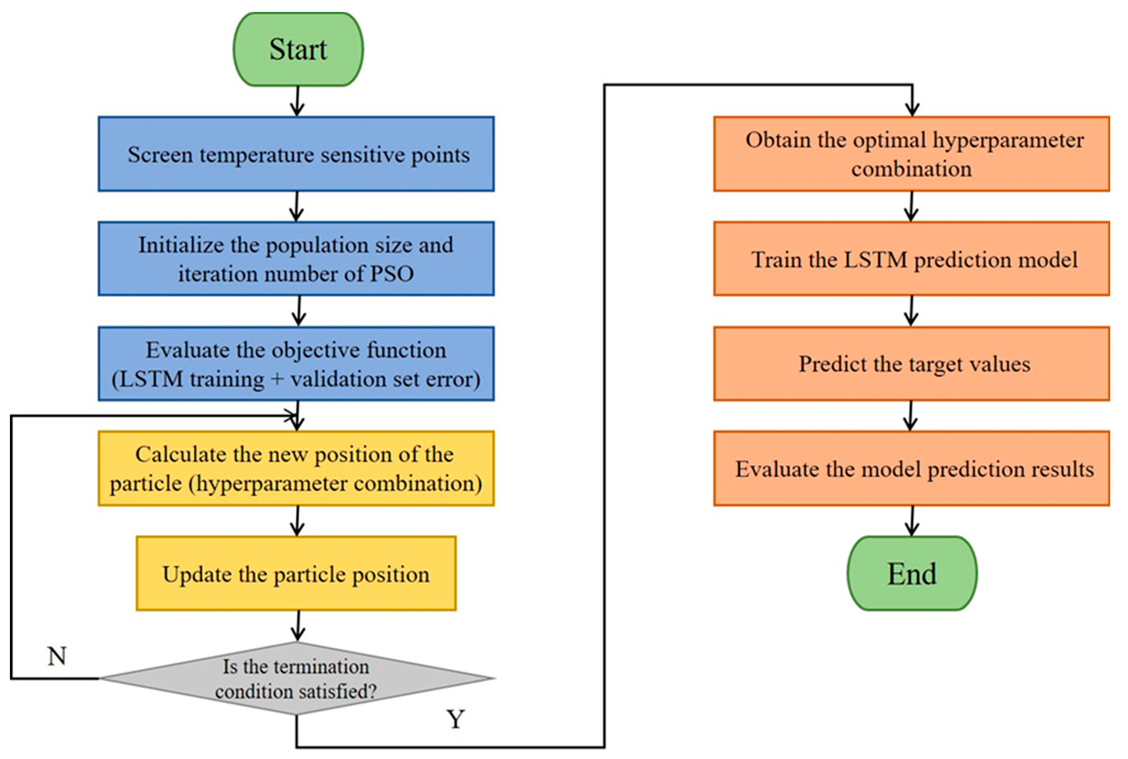
The thermal-error prediction model proposed in this paper (hereafter referred to as the PSO-LSTM model) consists of a Particle Swarm Optimization (PSO) algorithm and a Long Short-Term Memory (LSTM) prediction network. Benefiting from its simple structure and strong global search capability, the PSO algorithm is used to identify the optimal combination of LSTM hyperparameters—including the number of hidden units, initial learning rate, temporal window size, and regularization coefficient—in order to enhance the model’s predictive accuracy. The optimization workflow is illustrated in
Figure 1.
2.1. Temperature-Sensitive Point Selection
To establish an accurate regression mapping between thermal error and temperature sensors, reduce multicollinearity among measurement points, and improve model accuracy, fuzzy clustering analysis and global sensitivity analysis are employed to select temperature-sensitive points on the machine tool. In this study, the 19 temperature measurement points on the machine tool are grouped into two clusters via fuzzy clustering. The main theoretical formulations are as follows:
(1) Let represent a set of key monitoring variables and represent the observations of variable. The correlation coefficient between the monitoring variables is expressed as
where
Construct the fuzzy similarity matrix R from and apply the square-mean transitive closure to obtain the fuzzy-equivalence matrix , defined as t(R) = R^(2^k).
(2) Determine the threshold
, and classify the monitoring variables using the fuzzy equivalence matrix
. For
, define
Let be the cut matrix of at the level. Therefore, , where indicates that variables and belong to the same class.
Next, global sensitivity analysis is used to calculate the correlation between the two temperature measurement points obtained from fuzzy clustering analysis and the thermal error. The temperature measurement point with the highest correlation in each class is identified as the temperature-sensitive point for that class. Ultimately, two temperature-sensitive points for the machine tool are selected. The global sensitivity index calculation formula is as follows:
In the formula, represents the global sensitivity index of the I temperature measurement point, represents the instantaneous sensitivity coefficient of the I temperature measurement point at the K sample, and represents the length of the time window. Based on Equation (3), the global sensitivity index of the dependent variable with respect to different input variable can be sequentially calculated, thereby analyzing the importance of different input variables to the dependent variable .
2.2. Long Short-Term Memory (LSTM) Network
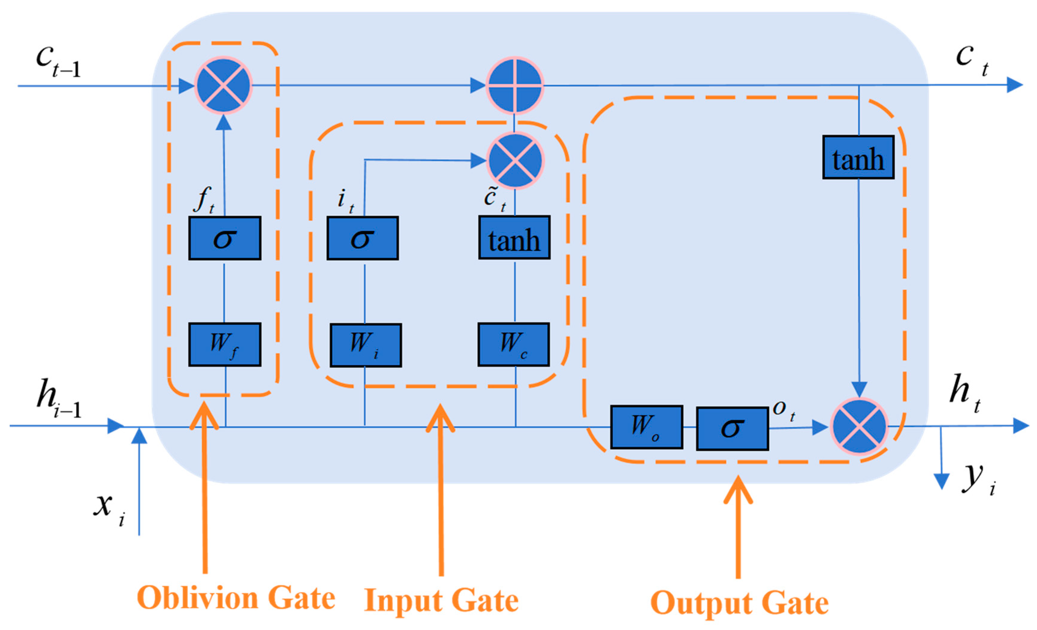
Long Short-Term Memory (LSTM) networks are a specialized form of Recurrent Neural Networks (RNNs). Traditional RNNs often encounter vanishing or exploding gradient problems when processing long sequences, which can prevent successful training and impair learning. LSTM networks resolve these gradient issues by incorporating gated structures and memory cells that precisely regulate information flow, thereby maintaining effective gradient propagation [
31]. The core of an LSTM cell is its cell state, depicted as a horizontal “conveyor belt” running through the cell with minimal branching. Three gates—the forget gate, input gate, and output gate—control the retention, updating, and output of information within the cell state. Consequently, an LSTM can preserve complete information over extended sequences and update that information to sustain memory across time steps. Leveraging these features, LSTMs can handle variable-length time series, capture long-term dependencies, and dynamically retain pa3t information while learning new patterns.
Figure 2 illustrates the structure of an LSTM cell. As shown, upon receiving input, the cell first removes unimportant information via the forget gate, which is computed as follows:
Here, represents the forget gate, is the activation function, is the weight matrix of the forget gate, is the output from the previous time step , is the current input, and is the bias vector.
Next, the input gate selects valuable information and adds it to the network while generating new cell information to be filtered. This process can be represented as follows:
where
and
are the intermediate values during the input gate and calculation process,
and
are the weight matrices for the input gate and internal state, and
and
are the biases for the input gate and internal state.
After processing through the forget gate and input gate, the cell state information is updated. The updated cell state
can be represented as follows:
Here, and represent the cell states at the current time step and the previous time step , respectively.
The updated cell state is passed through the output gate to generate the network output. First, the output gate activation
is computed using the activation function
to determine which information to emit. Next, the cell state
is processed by the tanh activation function and multiplied by the output weight matrix
to produce the final output
. The corresponding equations are as follows:
These equations reveal the internal computation of an LSTM cell, where each time-step output depends on prior inputs and cell states, enabling the network to handle variable-length sequences and capture long-term dependencies when forecasting future values.
This paper selects the mean squared error as the evaluation function of the neural network model, and its formula is as follows:
In the formula, yi is the predicted output result of the network model; ti is the expected output result of the network model; and p is the number of samples.
2.3. PSO-Based Hyperparameter Optimization for LSTM
This study employs Particle Swarm Optimization (PSO) to tune LSTM hyperparameters, specifically the learning rate and the number of hidden-layer neurons. In the PSO algorithm, each particle encodes three attributes—fitness, position, and velocity—where the position denotes a candidate solution’s coordinates in the search space, the velocity indicates its search direction and magnitude, and the fitness value evaluates the solution’s quality. During optimization, particles explore the search space from randomly assigned initial positions and velocities, each representing a possible solution. Thereafter, particles share their personal bests and the swarm’s global best to iteratively update their states, ultimately converging to the global optimum [
32].
Let
particles form a swarm
in a
dimensional search space. The position and velocity of the
i particle are denoted by
and
, respectively. Based on fitness evaluations, the personal best position of the
particle is
, and the global best position of the swarm is
. The update equations for the
particle’s velocity and position at iteration
t are given by
In the formula,
represents the algorithm’s iteration count; ω is the inertia weight, which determines the relationship between the particle’s velocity at the next time step and its current velocity;
and
are learning factors, primarily used to adjust the particle’s search capability;
and
are random numbers between 0 and 1, primarily used to enhance the particle’s random search ability. The search process of the algorithm is summarized in
Figure 3 [
33].
To ensure equivalence and homogeneity among various factors, the sample data must be processed into dimensionless normalized form. Therefore, this study employs the Z-score method to uniformly normalize the model data:
where
and
represent the sample data and its mean,
and
denote the standard deviation and the normalized value, respectively, and
is the number of samples.
2.4. Error Compensation Implementation Methods
2.4.1. Origin Translation Method
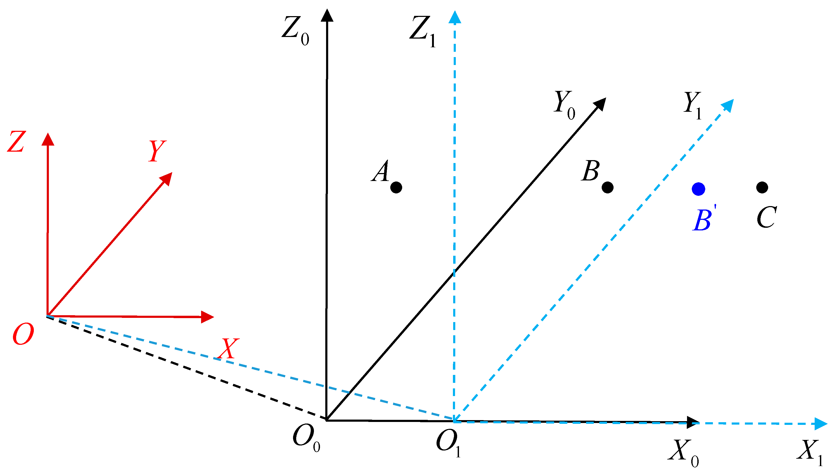
In the specific implementation process of real-time error compensation for machine tools, the feedback interruption method and the origin translation method are currently the two main compensation implementation methods. The compensation method used in this paper is based on the origin translation method. Using
Figure 4 as an example, the error compensation process based on the origin translation method is explained. Poin
is the fixed reference point of the machine tool, also known as the mechanical origin. The coordinate system oxyz with point
as the origin is referred to as the mechanical reference coordinate system. During the initial stage of machining, the coordinate system
with point
as the origin is referred to as the original machining coordinate system.
In the original coordinate system the initial position of the cutting tool is at point . After receiving the machining program instructions, the tool will move to point according to the machining instructions. However, due to machining errors, the cutting tool actually moves to point . Thus, can represent the machining error of the machine tool before compensation. In order to reduce machining errors, the machine tool’s system uses the origin translation method to perform a reverse shift in the origin coordinates. The shifted coordinate system origin moves from point to point , and the coordinate system with point as the origin is referred to as the new compensated machining coordinate system. In the new coordinate system , the actual position where the machine tool moves changes from point to point . The machine tool’s compensated actual machining error is reduced from to , thus achieving the precision compensation effect of the machine tool.
2.4.2. Application Process of the CNC System Temperature Compensation Function
To make the thermal error prediction model applicable to real-world scenarios, this paper developed a standalone temperature acquisition and thermal error compensation system. This system, implemented on an industrial computer, communicates with and feeds compensation data directly to the SINUMERIK 828D CNC system. The following section introduces the application process of the temperature compensation function of the SINUMERIK 828D CNC system.
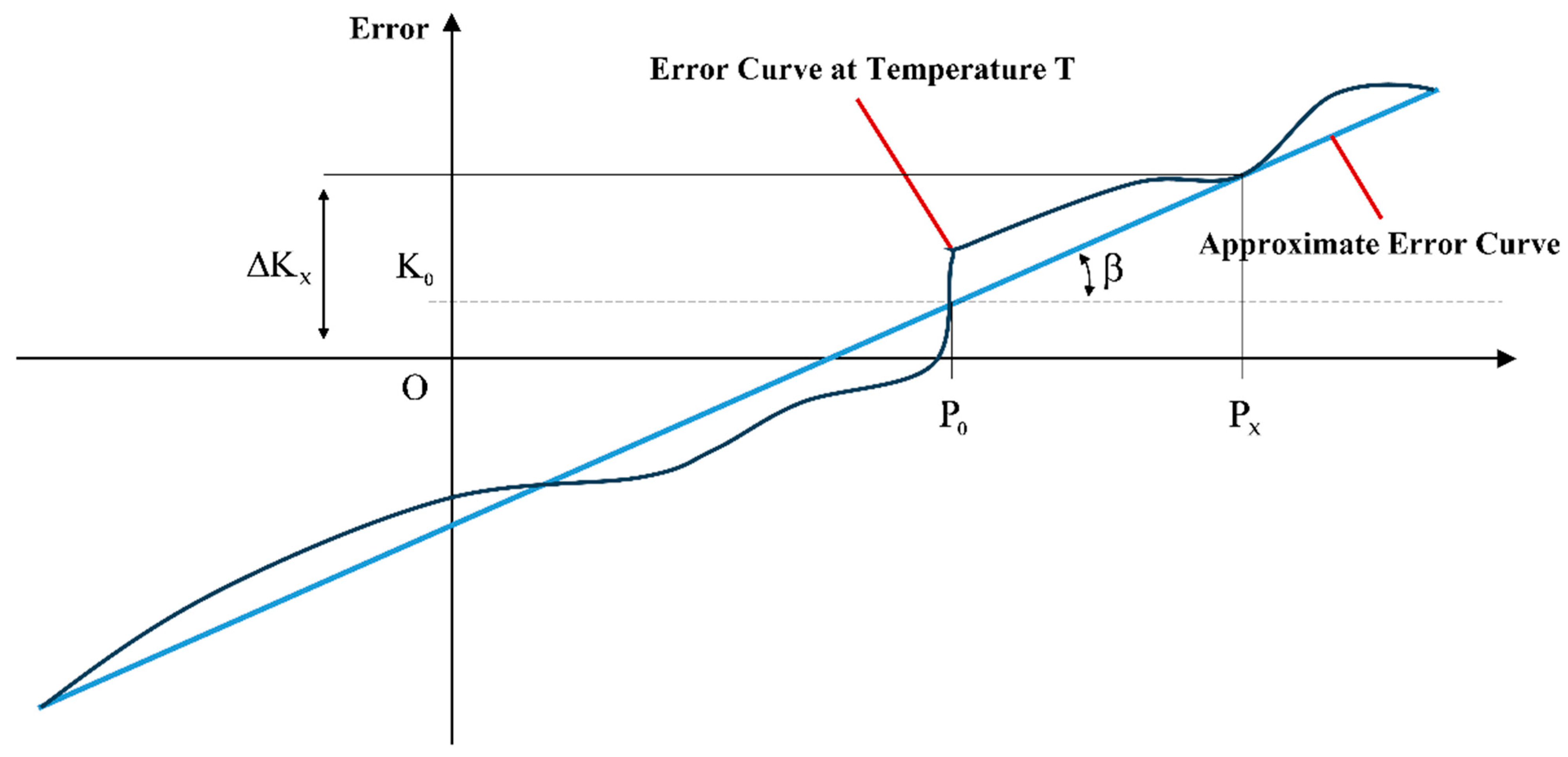
Figure 5 shows the positioning error curve of the
machine tool’s
X-axis at temperature
. In the figure,
represents a reference point at a specific location on the
X-axis. When the temperature changes to
T, the displacement error of reference point
is measured as
. The displacement error
at other points
during temperature changes can be calculated based on the slope TAN at temperature
T, the position of reference point
, and the displacement error
:
In the equation,
is the reference point;
is the actual position point on the X feed axis;
is the temperature compensation value at the reference point
;
is the error value at reference point
at temperature T;
is the temperature compensation coefficient, obtained from the slope of the error curve.
In the equation, is the initial temperature at the relevant position point; is the highest temperature variation at the relevant position point; is the maximum temperature coefficient.
4. PSO-LSTM-Based Thermal Error Prediction for the T55II-500
4.1. Identification and Optimization of Temperature Monitoring Point
Temperature sensitive points not only accurately characterize the machine tool’s thermal behavior but also reduce data redundancy and mitigate collinearity among measurement points, thereby improving modeling efficiency and prediction accuracy. In this study, fuzzy clustering analysis and global sensitivity analysis were applied to the temperature rise and thermal error datasets to identify the most temperature sensitive points.
Table 3 presents the fuzzy equivalence matrix for all 19 monitoring points. Using the F test, the F statistic corresponding to each λ value was computed; the results are shown in
Table 4. The results indicate that at λ = 0.946, the F statistic reaches its maximum, yielding the optimal clustering. Based on this threshold, the 19 temperature monitoring points were divided into two clusters, as shown in
Table 5.
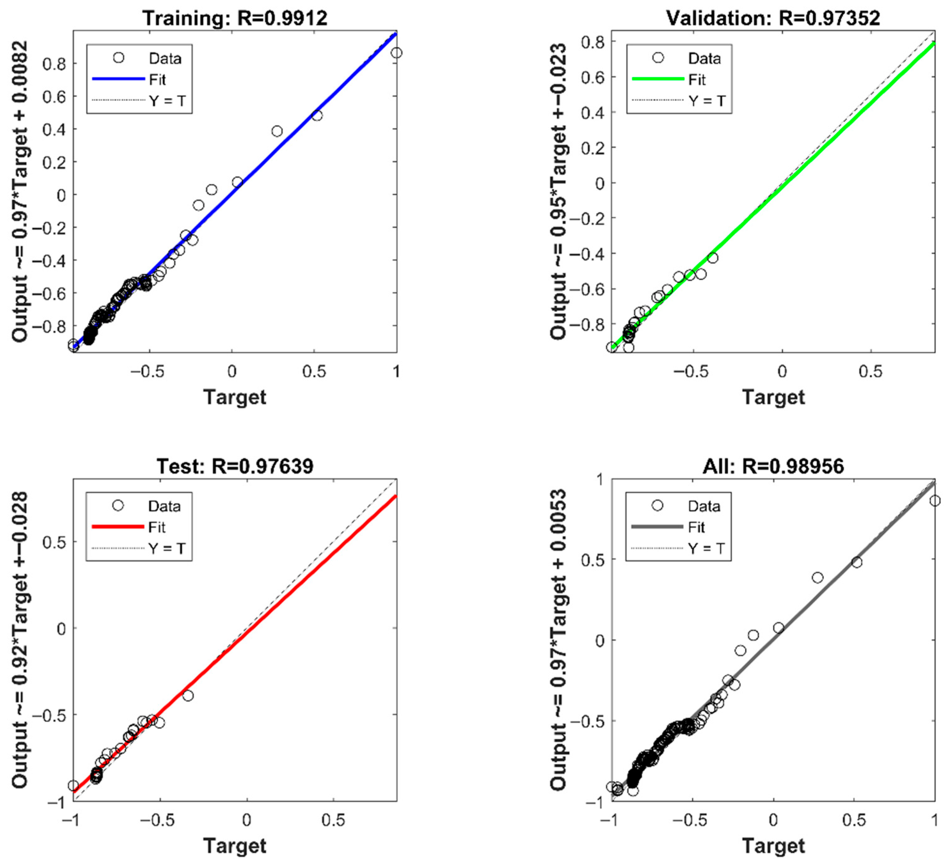
To determine the optimal point within each cluster, a global sensitivity analysis was performed on all 19 monitoring points. The procedure was as follows: based on the thermal characteristic test data, a dataset of 200 samples was constructed, using each point’s temperature and its increment as inputs and the relative increment of thermal error as the output (180 samples for training and 20 for validation). Prior to training, both inputs (temperature and increment) and outputs (relative thermal error increment) were normalized to eliminate scale and unit discrepancies. A neural network model was then trained on these samples; as shown in
Figure 10, the resulting models achieved R squared values exceeding 95%, indicating high accuracy and effectively capturing the mapping between thermal error and temperature measurements. These models serve to quantify each point’s influence on thermal error and support the selection of optimal monitoring points.
To identify the best point in each cluster, the sample data were further processed using global sensitivity analysis. Specifically, for each monitoring point, its input-variable increment was set to zero—thereby nullifying its perturbation effect—to generate a new sample set for that point. After processing, the modified samples were input into the trained neural network to produce outputs
Defining
as the baseline output, the change
was computed, and according to Equation (3), the global sensitivity index
for each temperature point was calculated. The global sensitivity indices for the 19 monitoring points on the T55II-500 are presented in
Table 6. The optimal point in the first cluster was T18 (index = 0.8681), and in the second cluster T2 (index = 0.9670). Consequently, points T2 and T18 were selected as the key monitoring locations for thermal-error modeling.
4.2. Thermal-Error Modeling of the T55II-500 CNC Machine Tool
The PSO LSTM thermal error prediction model comprises two main components: a Particle Swarm Optimization (PSO) algorithm for hyperparameter optimization and a Long Short-Term Memory (LSTM) network dedicated to thermal error prediction.
For the PSO LSTM network, temperature readings from points 2 and 18 served as inputs, and the predicted thermal error as the output. The input layer comprised three nodes, while both the output layer and the single hidden layer each contained one node. Of the 420 collected samples of machine tool temperatures and thermal errors, the first 360 were used for training and the remaining 60 for testing and validation. To enhance predictive performance, input and output datasets were normalized according to Equations (13)–(15). During LSTM training, the maximum number of iterations was set to 200, Mean Squared Error (MSE) was adopted as the evaluation metric, and the Adam optimizer was employed. The PSO algorithm was used to globally optimize the learning rate and hidden layer size. The swarm size was set to 40; the learning rate ranged from 0.01 to 0.15; the hidden layer neurons ranged from 1 to 200; acceleration coefficients c1 and c2 were both set to 2; the inertia weight linearly decreased from 1.2 to 0.8 over 30 iterations.
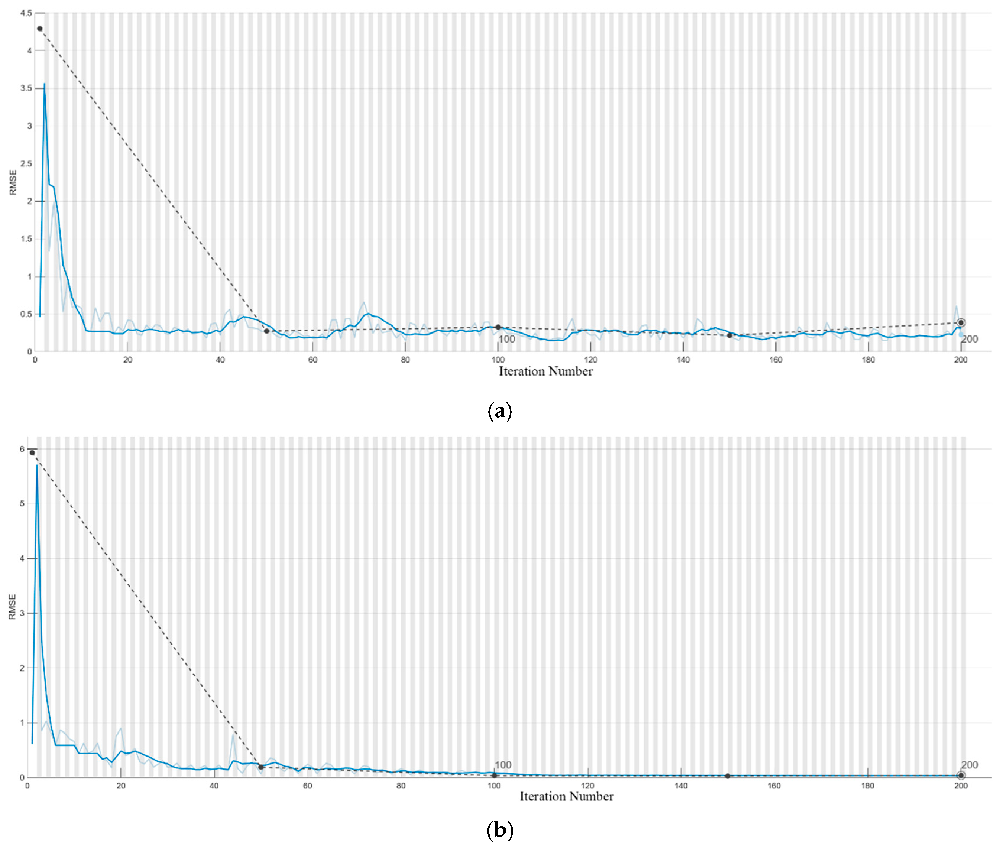
This study performed thermal error modeling of the T55II 500 CNC machine using a PSO LSTM network, with all model training conducted on the MATLAB R2023b platform. PSO yielded an optimal learning rate of 0.0941 and a hidden-layer size of 45 neurons.
Figure 11 depicts the iterative evolution of the optimal particle in the PSO algorithm.
To evaluate the optimization effect of the Particle Swarm Optimization (PSO) algorithm on the LSTM neural network, this paper conducts thermal error modeling and training on the basic LSTM neural network using the same sample dataset, network architecture, and parameter settings, aiming to compare and analyze the differences in prediction performance of the thermal error models before and after hyperparameter optimization.
Figure 12 shows the training convergence curves of the PSO-LSTM and LSTM neural network thermal error prediction models. It can be seen from the figure that as the number of iterations increases, the training accuracy of both the PSO-LSTM and LSTM neural network models continues to improve, and the PSO-LSTM model has a higher convergence accuracy. This indicates that the PSO-LSTM model has good learning ability and can effectively extract feature information and data patterns from the training samples.
4.3. Result Analysis and Comparison
The trained thermal-error models were validated using the test set.
Figure 13 shows the prediction comparison results and residual curves of the PSO-LSTM and LSTM neural network thermal error models. The PSO-LSTM predictions align almost perfectly with the measurements—particularly in the 10–45 min interval, where fluctuations are minimal and the fit is more consistent. Although the basic LSTM can predict thermal error reasonably well, it exhibits large deviations in several time segments. PSO-LSTM residuals largely remain within ±3 μm and fluctuate smoothly, whereas the LSTM model displays pronounced deviations and even sustained high errors in certain intervals. These comparisons indicate that the unoptimized LSTM is overly sensitive to operating-condition changes and lacks robustness, while PSO-LSTM offers greater stability across varying temperature-rise profiles. The underlying reason is that conventional LSTM models often rely on manual tuning or grid search for hyperparameters, making them prone to local optima, and their predictive performance heavily depends on hyperparameter choice. Integrating PSO enhances hyperparameter optimization by using swarm intelligence to explore the global solution space, facilitating the discovery of parameter sets that minimize error and maximize generalization. Moreover, because thermal error accumulates slowly, exhibits nonlinear trends, and is susceptible to early-stage temperature disturbances, an LSTM without proper tuning struggles to capture long-term dependencies; PSO-optimized LSTM, however, exhibits improved modeling of both long-sequence dependencies and nonlinear behaviors.
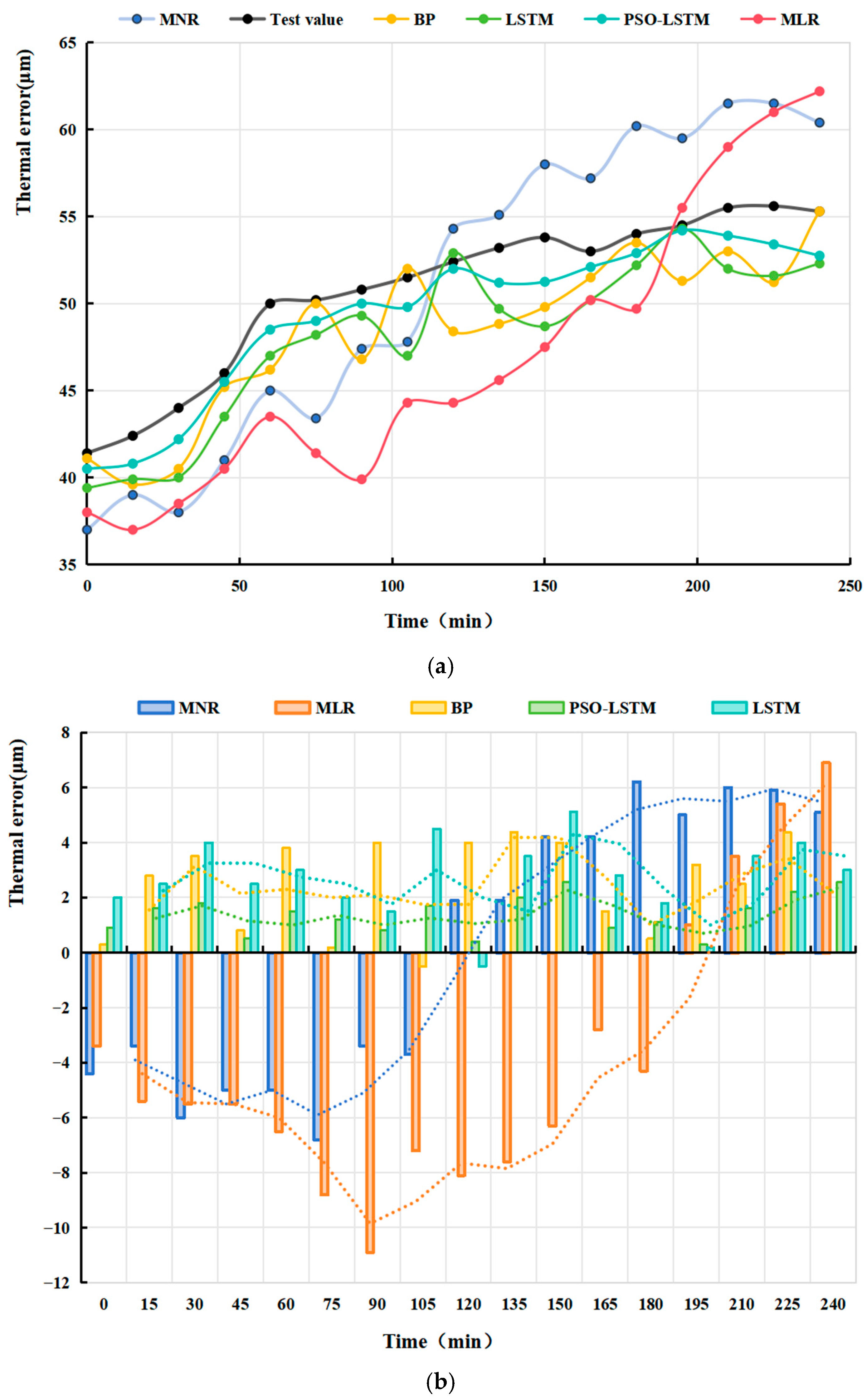
To validate the effectiveness and robustness of the proposed model and compare its performance with other models in this study, the data from
Section 3.2 were normalized and input into the models. The first 80% of the data were used as the training set, and the remaining 20% as the test set. The PSO results yielded a time window size of 5, a learning rate of 0.0941, and 45 units. For a fair comparison, the remaining three models were configured with the same structure. The prediction result curves of each model are shown in
Figure 14.
Error analysis metrics for five thermal-error models are summarized in
Table 7. Among the established models, the MLR thermal-error model had a relative error of 10.67%, while the other models had relative errors below 10%, indicating that all thermal-error models possess some predictive capability. Among the models, the PSO-LSTM thermal-error model performed the best, with a relative error of 2.22%, demonstrating high prediction accuracy. The LSTM and BP thermal-error models followed, with relative errors of 4.29% and 3.84%, respectively, while the MNR and MLR models had relative errors of 9.68% and 10.67%. Regarding residual data, the average and maximum residuals of all models were kept within 15 μm, with the PSO-LSTM model showing the best residual performance: an average residual of 1.39 μm and a maximum residual of 2.55 μm. This indicates that its predictions not only exhibit low bias but also have minimal fluctuation, with the error distribution being more concentrated and stable. The PSO LSTM thermal error model’s mean squared error (MSE) was 2.52 μm, indicating minimal error fluctuations throughout the prediction process. The model output was smooth and stable, demonstrating good engineering applicability and robustness.
The reasons behind these results can be summarized as follows:
- (1)
Compared to static models like MLR and MNR, the LSTM and PSO-LSTM thermal error prediction models can effectively capture long-term dependencies in time series, making them especially suitable for dynamic problems like CNC machine tool thermal error, which evolves slowly over time. This significantly enhances their ability to model the evolution of thermal error.
- (2)
While BP can handle nonlinearity, it cannot model time dependencies, and its training is influenced by initial weights, often falling into local optima. In contrast, PSO’s global search capability allows LSTM to avoid such issues.
- (3)
MLR is a purely linear model, and MNR is a weakly nonlinear model, making them inadequate for modeling the complex nonlinear and dynamic characteristics of thermal error evolution. PSO-LSTM combines both time series modeling and nonlinear modeling, fundamentally overcoming the modeling capability bottleneck.
Therefore, the PSO-LSTM model combines LSTM’s ability to handle time series data with PSO’s advantages in hyperparameter optimization, improving the model’s ability to capture the nonlinear and dynamic characteristics of machine tool thermal error. It shows strong potential for engineering applications.
4.4. Thermal-Error Compensation System Based on the SINUMERIK 828D CNC
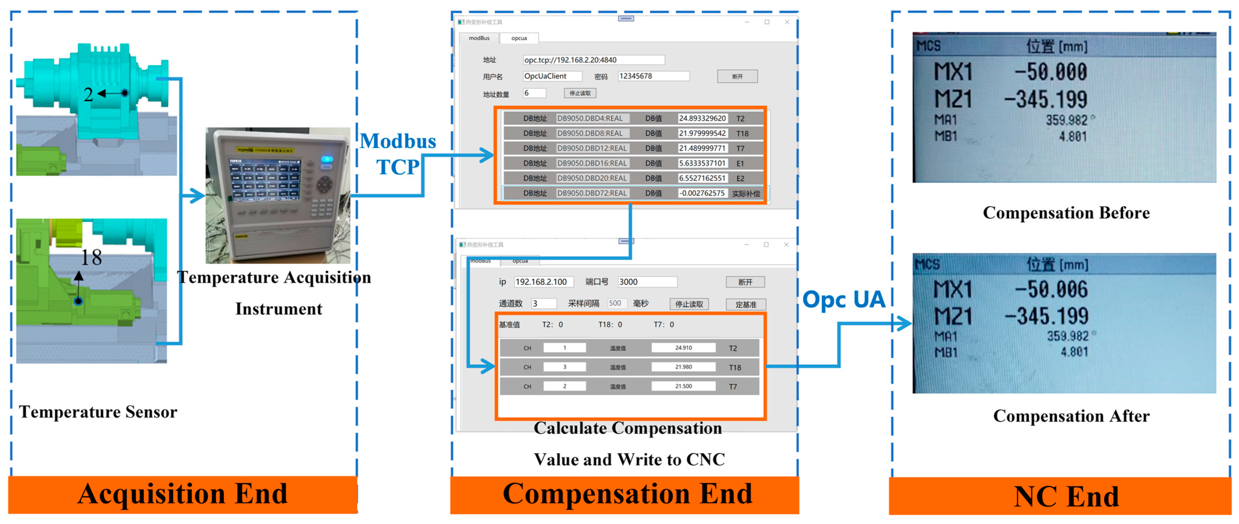
Error compensation technology is implemented by establishing a dedicated error compensation control system for machine tools. This system predicts the thermal errors of the machine tool in real time and transmits compensation signals to the servo drives, thereby controlling each axis to execute the required corrective movements. To meet the needs of practical applications, this study has developed temperature acquisition and thermal error compensation software on the SINUMERIK 828D CNC platform.
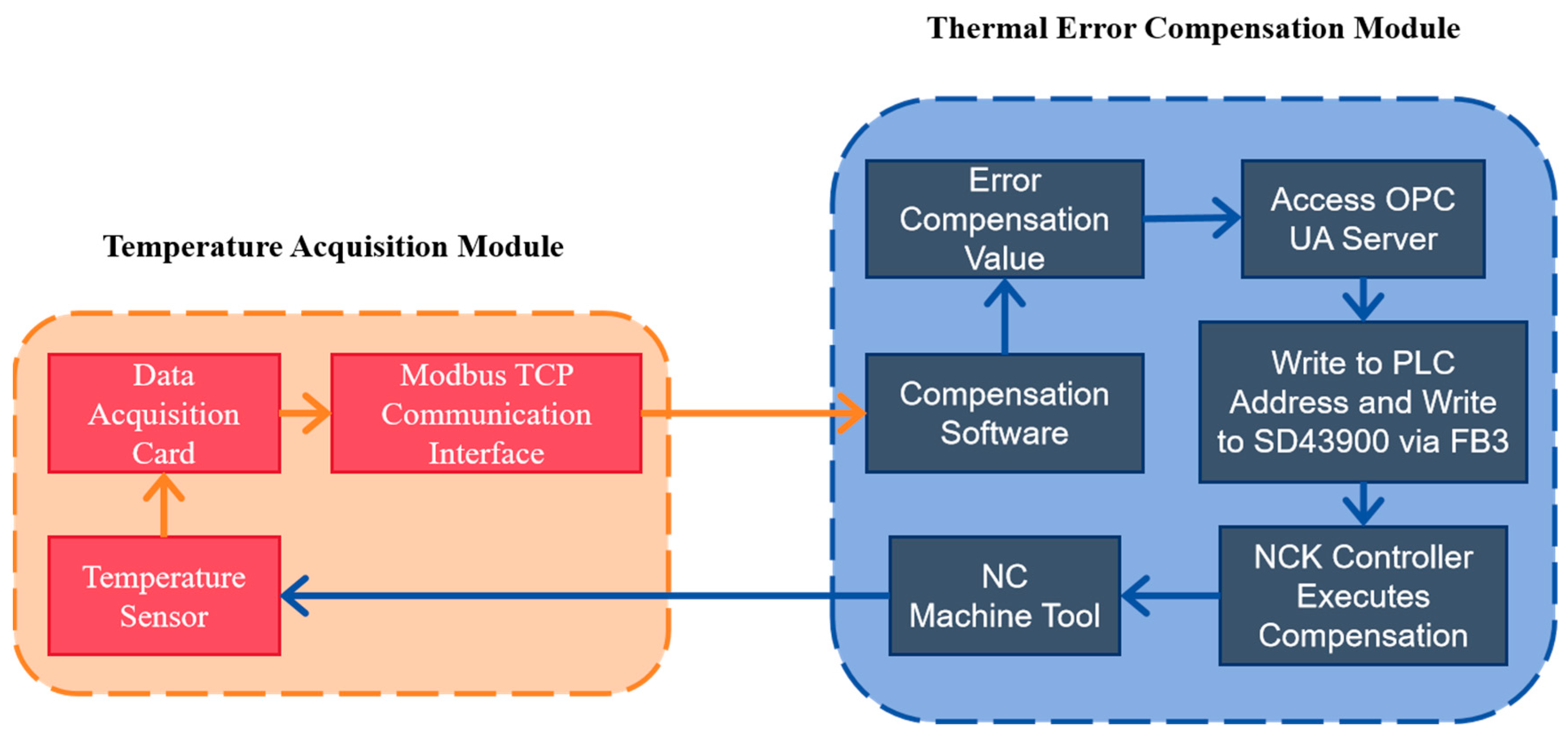
Figure 15 shows the implementation schematic diagram of the thermal error compensation system based on SINUMERIK 828D. During the compensation process, temperature data are first acquired from the machine tool’s monitoring points through sensors and data acquisition cards; then, the data are sent to the compensation software via the Modbus TCP protocol to calculate the required correction values; finally, these correction values are written into the PLC (Programmable Logic Controller) through the OPC UA server, and then forwarded by the PLC to the CNC system to trigger its built-in thermal compensation program.
Figure 16 shows the specific compensation implementation process of the SINUMERIK 828D thermal error compensation system. The data transmission process in the SINUMERIK 828D based thermal error compensation system comprises three modules:
- (1)
The temperature acquisition module, using sensors placed at critical points on the machine, monitors temperature changes in real time and transmits this data via Modbus TCP to the error compensation module for further processing and analysis.
- (2)
Under the Visual Studio environment, a C# program was developed to communicate with the CNC machine’s PLC over Modbus TCP. The error compensation module uses the established thermal error model and relevant inputs to compute compensation values in real time. These values are then standardized—converting units and data types—via the PLC control program. Finally, the processed compensation values are written into the NC system through the OPC UA server interface.
- (3)
Using the PLC Programming Tool as the development environment, the CNC machine’s PLC program was written and debugged. Data exchange with the CNC system is handled via FB2 and FB3 function blocks: FB2 reads system variables and drive parameters, while FB3 writes them. The PLC then writes the compensation values into register SD43900 to invoke the built in temperature compensation feature. During compensation, the CNC system adds the correction value to its setpoint, causing the servo to drive the feed axis in the opposite direction (a positive compensation value yields a negative feed motion).
To validate the compensation effect of the thermal error compensation system, error compensation tests were conducted on the T55II-500 CNC machine tool. To verify the stability of the thermal error compensation system, three different environmental temperature conditions were designed in this study, including: a near-constant temperature condition (19.34–20.36 °C), a warm natural ventilation condition (20.63–22.13 °C), and a variable temperature condition with a wider range (18.64–28.24 °C). These conditions were designed to validate the compensation system’s stability under different thermal loads and environmental fluctuations.
Table 8 shows the environmental temperature conditions.
Table 9 shows the machining conditions of the machine tool.
Through thermal error compensation tests, machining error data for the CNC machine tool before and after the activation of the thermal error compensation system were measured.
Table 10 presents the verification results of the CNC machine tool’s thermal error compensation system under three temperature conditions.
Figure 17 shows the thermal error compensation effectiveness of the CNC machine tools under different temperature conditions. The test results show that the environmental temperature has a significant impact on the machine tool’s thermal error. Under temperature variation conditions, the machine tool’s thermal error reached a maximum of 67 μm. Under three different environmental temperature conditions, the machining errors after system compensation were all controlled within 10 μm, and the machine tool’s machining precision was improved by up to 88%. This indicates that the thermal error compensation system for the SINUMERIK 828D CNC machine tool, designed in this paper, significantly improves the machining precision, demonstrating excellent practical application results.
5. Conclusions and Future Work
This paper proposes a data-driven thermal error prediction model for the T55II-500 CNC machine tool based on Particle Swarm Optimization—Long Short-Term Memory Network (PSO-LSTM). This method can accurately predict the thermal errors of CNC machine tools, providing a basis for thermal error compensation and helping to improve machining accuracy. By using experimentally obtained thermal error data and comparing the performance of different thermal error prediction models under various working environments, the effectiveness and robustness of the proposed model are verified. The main conclusions are as follows:
- (1)
A thermal error model for the T55II-500 CNC machine based on PSO-LSTM was proposed and validated through thermal characteristic experiments. The comparison between the PSO-LSTM model and experimental results shows that the model can accurately predict the thermal error of the T55II-500 CNC machine, laying the foundation for thermal error compensation. Further verification of the model’s robustness was carried out through experiments in random and controlled-temperature environments. Comparison of the predicted and experimental results shows that the PSO-LSTM model not only predicts thermal errors accurately but also maintains stable and satisfactory robustness under complex operating conditions.
- (2)
A comparison between the proposed model and traditional models was made. In this study on the thermal-error prediction model for the T55II-500 CNC machine, the PSO-LSTM model demonstrated higher accuracy and lower error compared to the backpropagation neural network (BP), multiple linear regression (MLR), long short-term memory (LSTM) network, and polynomial nonlinear regression (MNR) models. The PSO-LSTM model showed the smallest relative error, average residual, mean square error, and maximum residual values, indicating superior performance.
Although the thermal error prediction model proposed in this paper has been established and applied to high-precision machine tools, the performance of the model in relation to the machine tool under different work intensities and spindle speeds has not yet been tested.
Future research will utilize the established model to conduct thermal error compensation experiments under varying working intensities and spindle speeds, systematically validating the method’s effectiveness. As current validation was limited to a single platform (T55II-500 equipped with SINUMERIK 828D), subsequent work needs to verify the model’s generalizability across different machine tool architectures and CNC systems. Furthermore, we will develop enhanced models that explicitly integrate multi-source information, incorporating not only temperature variables but also critical process parameters including coolant flow rates, spindle loads, and tool wear conditions. This comprehensive approach will significantly improve model adaptability in complex working conditions.
To ensure robust performance in practical industrial environments, we will incorporate dedicated anomaly detection modules to handle severe data abnormalities arising from sensor failures or unexpected operational conditions. Additionally, we will investigate adaptive mechanisms specifically designed to counteract performance degradation in dynamic manufacturing scenarios.
Due to experimental cycle limitations, the model’s adaptability to long-term machine tool aging effects remains unverified. Follow-up studies will implement long-term tracking experiments combined with online model update algorithms to systematically investigate the impact of time-varying factors on model performance. The development of these adaptive mechanisms will be crucial for maintaining model accuracy throughout the machine tool’s lifecycle. Simultaneously, to address the lack of uncertainty quantification in the current deterministic prediction approach, advanced methods such as Bayesian neural networks or Monte Carlo Dropout will be introduced to establish reliable confidence intervals for predictions, thereby enhancing decision-support capabilities in risk-sensitive scenarios.
