Adaptive Prediction of Compressor Cylinder Pressure Dynamics Using a Physics-Guided VAE-CNN State Space Model

Abstract

Air compressor valves are prone to mechanical wear and elastic fatigue during long-term operation, often leading to poor sealing or leakage. Such leakage is a typical failure mode of reciprocating compressors, introducing strong nonlinearities into cylinder pressure dynamics and significantly increasing the difficulty of state monitoring. To address this issue, this paper presents an adaptive prediction method for compressor cylinder pressure dynamics under valve leakage failure, based on a physics-guided Variational Autoencoder Convolutional Neural Network State Space Model (VAE-CNN-SSM). In this framework, a VAE with embedded physical information is employed to construct the state equation and generate latent variables reflecting valve motion degradation, while a CNN-based observation equation is established to map latent states to cylinder pressure. This hybrid modeling strategy enables accurate prediction of cylinder pressure dynamics and effective characterization of valve degradation behaviors under valve leakage failure conditions. Comparative experiments against conventional models demonstrate that the proposed method achieves superior predictive accuracy, robustness, and generalization. These findings provide a new approach for analyzing valve leakage failures and offer technical support for condition monitoring, health management, and predictive maintenance of reciprocating compressors.

1. Introduction

The reciprocating compressor is a vital component in industrial manufacturing, playing a crucial role in daily operations by providing compressed air power for various production processes. However, during long-term service, leakage has become a key factor affecting the efficiency and reliability of compressors. The effectiveness of sealing is essential to the efficiency, safety, and stability of fluid machinery. Recent studies have reported progress in leakage reduction and sealing performance enhancement for fluid equipment [1,2]. Despite these advances, valve-induced leakage remains one of the most challenging issues in reciprocating compressors, as it directly affects cylinder pressure dynamics and overall system performance. Leakage not only undermines the accuracy of operating status prediction but also leads to deviations in health assessment, which may cause energy waste and increased operating costs, thereby compromising the overall performance of the production system. In most cases, compressor leakage arises from incomplete valve closure. As the key element of reciprocating compressors, reed valves open and close under the pressure difference between the two sides. Once leakage occurs, this pressure difference is altered, resulting in delayed opening and premature closing of the valve [3]. Such valve leakage introduces strong nonlinearities into cylinder pressure dynamics, which greatly increases the difficulty of monitoring compressor operating conditions. Therefore, studying the impact of valve leakage on cylinder dynamics is of great significance for compressor health management and predictive maintenance. Furthermore, since valve motion states under leakage are implicit and cannot be directly measured by conventional sensors, there is a pressing need for adaptive prediction methods that can capture nonlinear pressure evolution across diverse operating scenarios, ensuring both accuracy and robustness in practical applications.

Modeling compressors is a direct method for understanding the operating status of air compressors. In recent years, scholars have conducted extensive research on compressor modeling, which can be divided into three types: The first type is a mathematical model established based on physical principles. Rigola et al. [4] established a numerical model for fully enclosed reciprocating compressors. Nagarajan et al. [5] established a mathematical model for reciprocating compressors, which can predict cylinder pressure, cylinder temperature, and air mass flow rate, and the simulation results are very similar to the experimental results. Mahmood et al. [6] established a zero-dimensional numerical model for reciprocating compressors, which considers piston motion, valve dynamics, and other mass flow rates, and simulates pressure and temperature at different degrees of valve leakage. Silva et al. [7] studied the impact of gas leakage in valves on compressor performance by establishing a simulation model. The results showed that even small valve leaks can significantly affect the efficiency of the compressor, and leakage from the exhaust valve can have a greater impact. Eihaj et al. [8] predicted the valve movement and cylinder pressure of the compressor by establishing a numerical model. Damle et al. [9] proposed an unstructured numerical simulation model for reciprocating compressors and compared it with experimental results, indicating good consistency between the numerical and experimental results.

Mathematical models are constructed based on clear physical mechanisms and have a rigorous theoretical foundation. This makes the model highly interpretable and reliable. However, for complex systems, the complexity of mathematical models is high, requiring a large number of parameters and equations. In applications, the computational cost of the model may be very high, which can affect the response speed of the system. The maintenance cost of the model is also high, and as the operating conditions change, the model needs to be constantly updated and rebuilt to adapt to new situations.

The second type is simulation software based on computer technology. With the development of technology and the improvement of computer performance, simulation software technology continues to evolve, and fluid structure interaction (FSI) simulation methods are gradually applied to the simulation of compressors. Wang et al. [10] established a three-dimensional fluid structure interaction model of a reciprocating compressor with a reed valve. The comparison between experimental and simulation results shows that the simulation results of the three-dimensional fluid structure interaction model of the compressor are reliable. Hwand [11] studied the behavioral characteristics of the exhaust valve of a linear compressor using a rigid body model of a reed valve and an FSI model. The results indicate that the simulated valve lift is consistent with the experimental results. Zhao et al. [12] proposed a three-dimensional computational fluid dynamics model for reciprocating compressors, which can simulate the motion of valve plates and predict pressure pulsation. Wang et al. [13] studied the valve oscillation and delayed closure problems of compressors at different speeds and valve parameters based on the FSI model. Wu et al. [14] conducted FSI model simulations on the suction valves on the piston and cylinder head of reciprocating compressors, and the results showed that they were relatively reliable. Bacak et al. [15] developed an FSI model for predicting the performance of reciprocating compressors and analyzing valve motion. This model exhibits excellent numerical stability.

Although simulation software can effectively handle complex systems and processes, provide comprehensive analysis and simulation, and perform extensive testing and analysis to adjust model parameters. However, simulation results are highly dependent on the accuracy of the established model, and if the model is not precise, misleading results may occur. And the simulation process involves a large amount of data and complex calculations, requiring a significant amount of computing resources, resulting in a lengthy calculation and analysis process.

The third type is based on artificial intelligence algorithm models: with the rapid development of artificial intelligence algorithms, their applications in various fields are becoming increasingly widespread. In the modeling process of compressors, models based on artificial intelligence algorithms provide a new perspective for performance analysis and prediction of compressors. This type of model utilizes machine learning and deep learning techniques to learn system features and patterns from a large amount of historical data, achieving accurate prediction of compressor operating status. Fu et al. [16] developed a model that combines Extreme Gradient Boosting (XGBoost) and mixed variational artificial bee colonies. This model is used to describe the mapping relationship between compressor operating parameters and performance parameters, achieving highly accurate and efficient prediction tasks. Belman et al. [17] constructed two models of reciprocating compressors, one based on physical foundations and the other based on artificial neural networks. The comparative experimental results indicate that physical models require assumptions, simplifications, and estimations of certain parameters in order to obtain them. Artificial neural network models can be directly created from measurement data and have higher prediction accuracy. Ledesma et al. [18] used artificial neural networks to model reciprocating compressors. Perform individual Artificial Neural Network (ANN) modeling for each energy parameter and obtain the optimal model parameters through optimization algorithms. Kumar et al. [19] developed a Gaussian regression model based on Bayesian optimization for performance prediction of screw compressors. Compared with support vector machines, artificial intelligence networks, and polynomial regression, the results show that the accuracy and inherent uncertainty quantification of this method are superior to other models. Ghorbanian et al. [20] applied various neural networks such as Generalized Regression Neural Network (GRNN), Rotating General Regression Neural Network (RGRNN), Radial Basis Function Network (RBFN), and Multilayer Perceptron (MLP) to predict the performance of compressors. The results showed that the MLP has extremely high efficiency in predicting compressor progress. Wang et al. [21] established a dual CNN model to reconstruct the pressure and temperature fields of a turbine under specific conditions, which has high accuracy and is more efficient than traditional simulation methods.

Artificial intelligence algorithms, especially deep learning techniques, have powerful capabilities to handle complex nonlinear relationships and high-dimensional data, particularly in complex systems that are difficult to accurately describe with traditional physical models. However, artificial intelligence methods have a high dependence on the quality and quantity of training data. Although deep learning models perform well in dealing with complex problems, their “black box” nature makes it difficult to explain the internal mechanisms of the model, limiting its interpretability.

The State Space Model is a mathematical model that can describe the changes of dynamic systems over time [22]. SSM constructs the system’s state variables separately from the observed variables, which not only characterizes the internal state of the system, but also reveals the relationship between the internal state of the system and external input and output variables. In recent years, it has been used by many scholars for fault diagnosis and prediction of mechanical equipment. Pedregal et al. [23] established a state detection system based on a state space model to predict the future state and failure probability of key turbines driving centrifugal compressors. Zhang et al. [24] proposed a fault diagnosis model based on discrete state space to identify the operating conditions of reciprocating compressors. This model can more robustly reflect their operating conditions and better complete fault detection. Ye et al. [25] developed an instantaneous response model for variable capacity refrigeration systems. Representing dynamic models such as evaporators and condensers in state space can provide a clearer understanding of their dynamic characteristics. Scholars have combined neural networks with SSM to achieve better performance. Skordilis et al. [26] developed a hybrid SSM based on multiple random layers. This model is capable of representing the evolution of system operating conditions and predicting equipment degradation over time. Liu et al. [27] used state space models and VAE to construct a deep probability time series prediction model. Integrating dynamic systems into the model using SSM to achieve high-precision prediction tasks. Zhou et al. [28] proposed a hybrid model that embeds neural networks into SSM to achieve real-time monitoring of bearing health status. The experimental results of batch accelerated degradation of bearings demonstrate the effectiveness and superiority of this method. And it indicates that the state space model can describe the influence of time-varying conditions.

In summary, to ensure both interpretability and accuracy, integrating deep learning with state-space models offers an effective approach for the adaptive prediction of compressor cylinder dynamics. However, it is extremely difficult to directly obtain real-time valve motion data under complex operating conditions when constructing a state equation that reflects valve operating status. Variables related to valve motion are typically implicit and cannot be accurately measured by conventional sensors. To address this challenge, this paper proposes a state-space model based on a Variational Autoencoder (VAE) and a Convolutional Neural Network (CNN) for adaptive prediction of compressor cylinder pressure dynamics. Specifically, the state equation is formulated using a VAE with embedded physical information. Leveraging the strong latent space modeling capability of the VAE [29], latent variables associated with valve motion states are generated to describe the underlying dynamic characteristics of the valve. Subsequently, a CNN-based observation equation is developed to extract complex features from cylinder pressure, enabling high-precision adaptive prediction of cylinder pressure evolution under nonlinear and leakage-affected conditions.

The main contributions of this paper are summarized as follows: (1) An adaptive prediction framework based on a VAE-CNN state space model is proposed to capture the dynamic characteristics of compressor cylinders, significantly enhancing prediction accuracy and generalization across multiple operating conditions. (2) A physics-guided VAE model is developed by embedding valve motion information into the state equation, which improves both the interpretability and predictive performance of the model. The remaining parts of this paper are organized as follows: Section 2 is an analysis of the problem of compressor valve leakage and related theories, Section 3 is an introduction based on model principles, Section 4 is an analysis of experimental details, Section 5 is result analysis, and Section 6 is a conclusion.

2. Problem Statement

2.1. Problem Analysis

The valve of a reciprocating compressor is a crucial component. During the compression, discharge, expansion, and suction processes of the compressor, valves control the suction and discharge of gas by opening and closing [13]. Therefore, the motion state of the valve has a significant impact on the health of the compressor and the motion characteristics of the cylinder. Once the valve leaks, it will directly affect the pressure change of the compressor cylinder. However, due to long-term use, valve wear, or material fatigue, the valve may deform and fail to fully close, resulting in leakage. This will cause a decrease in the effective pressure inside the cylinder, and at the same time, the movement state of the valve will also change, which will affect the movement process of the compressor [8]. The structure of the valve and the schematic diagram of the leakage are shown in Figure 1. Specifically, during the intake phase, the presence of leakage holes will cause backflow from the cylinder, resulting in a higher pressure level than normal, leading to delayed opening of the intake valve. As the pressure inside the cylinder increases, the airflow enters the cylinder through the hole during the intake process, resulting in an abnormal increase in cylinder pressure. This will cause the intake valve to close prematurely, thereby shortening the normal intake time. During the compression phase, due to the presence of leakage holes, high-pressure gas leaks out of the cylinder during the compression process, causing the pressure inside the cylinder to not increase as expected, which may delay the opening time of the exhaust valve. As the exhaust process progresses, high-pressure gas is discharged from the hole, causing a decrease in cylinder pressure and premature closure of the exhaust valve, leading to the early start of the expansion phase. The schematic diagram of pressure changes caused by valve leakage is shown in Figure 2.

Therefore, the nonlinear and complex pressure fluctuations caused by valve leakage greatly increase the difficulty of accurately predicting cylinder pressure. Traditional compressor modeling methods generally assume intact valve sealing, making it difficult to capture leakage-induced dynamics. Such irregular pressure variations not only reduce the accuracy of cylinder pressure prediction but also lead to deviations in overall system performance. Hence, in the adaptive prediction of compressor cylinder dynamics, it is essential to explicitly account for leakage effects in order to enhance both the accuracy and robustness of the model.

2.2. Mathematical Model

During the intake and exhaust process of the compressor cylinder, the intake and exhaust valves automatically open or close according to the pressure difference between the inside and outside, regulating the inflow and outflow of gas. According to Newton’s second law and reference [3], the motion formula of the reed valve can be obtained as follows:

$$M_v{\displaystyle \frac{d^2{h}_v}{d{t}^2}}=F_{vg}-F_{ve}+G_v-F_{vn}-F_{vv}$$

(1)

where $M_v$ is the mass of the reed valve, $h_v$ is the displacement of the reed valve at the center of the valve channel, $F_{vg}$ is the gas force, $F_{ve}$ is the elastic force of the reed valve, $G_v$ is the gravity of the reed valve, $F_{vn}$ is the gas resistance, $F_{vv}$ is the viscous force. Due to the fact that the gravity, gas resistance, and viscous force of the reed valve are much smaller than the elastic and gas forces, they can be ignored for the convenience of analysis.

The formula for gas force $F_{vg}$ is

$$F_{vg}=A_v\beta \left(p_{cy}-p_e\right)={\displaystyle \frac{\pi d^2\beta }{4}}\left(p_{cy}-p_e\right)$$

(2)

where $A_v$ is the area of the valve channel, $\beta$ is the gas thrust coefficient, and $d$ is the diameter of the valve channel, $p_{cy}$ is the pressure inside the cylinder, and $p_e$ is the exhaust pressure.

Assuming the reed valve is a cantilever beam, according to Hooke’s law, the elastic force is directly proportional to the formation, and the formula for the elastic force $F_{ve}$ is

$$F_{ve}=k·\left(h+h_0\right)$$

(3)

where $h$ is the valve lift, $h_0$ is the reserved pressure lift, and for the cantilever beam coefficient k, the general value is

$$k={\displaystyle \frac{3EI}{L^3}}$$

(4)

where $E$ is the elastic modulus of the reed valve, $I$ is the moment of inertia of the cross-section, and $L$ is the length of the reed valve.

Let the valve opening $\alpha ={\displaystyle \frac{h}{h_{max}}}$, then the differential equation of motion for the reed valve is

$${\displaystyle \frac{d^2\alpha }{d{\theta }^2}}={\displaystyle \frac{\pi d^2\beta }{4{M_v\mathsf{\omega }}^2{h}_{max}}}\left(p_{cy}-p_e\right)-{\displaystyle \frac{3EI\alpha }{{M_v\mathsf{\omega }}^2{L}^3}}-{\displaystyle \frac{3EI{h}_0}{{M_v\mathsf{\omega }}^2{h}_{max}{L}^3}}$$

(5)

where $h_{max}$ is the maximum lift of the valve, $\theta$ is the crankshaft rotation angle, and $\mathsf{\omega }$ is the rotational speed of the crankshaft.

3. Proposed Model

3.1. Framework

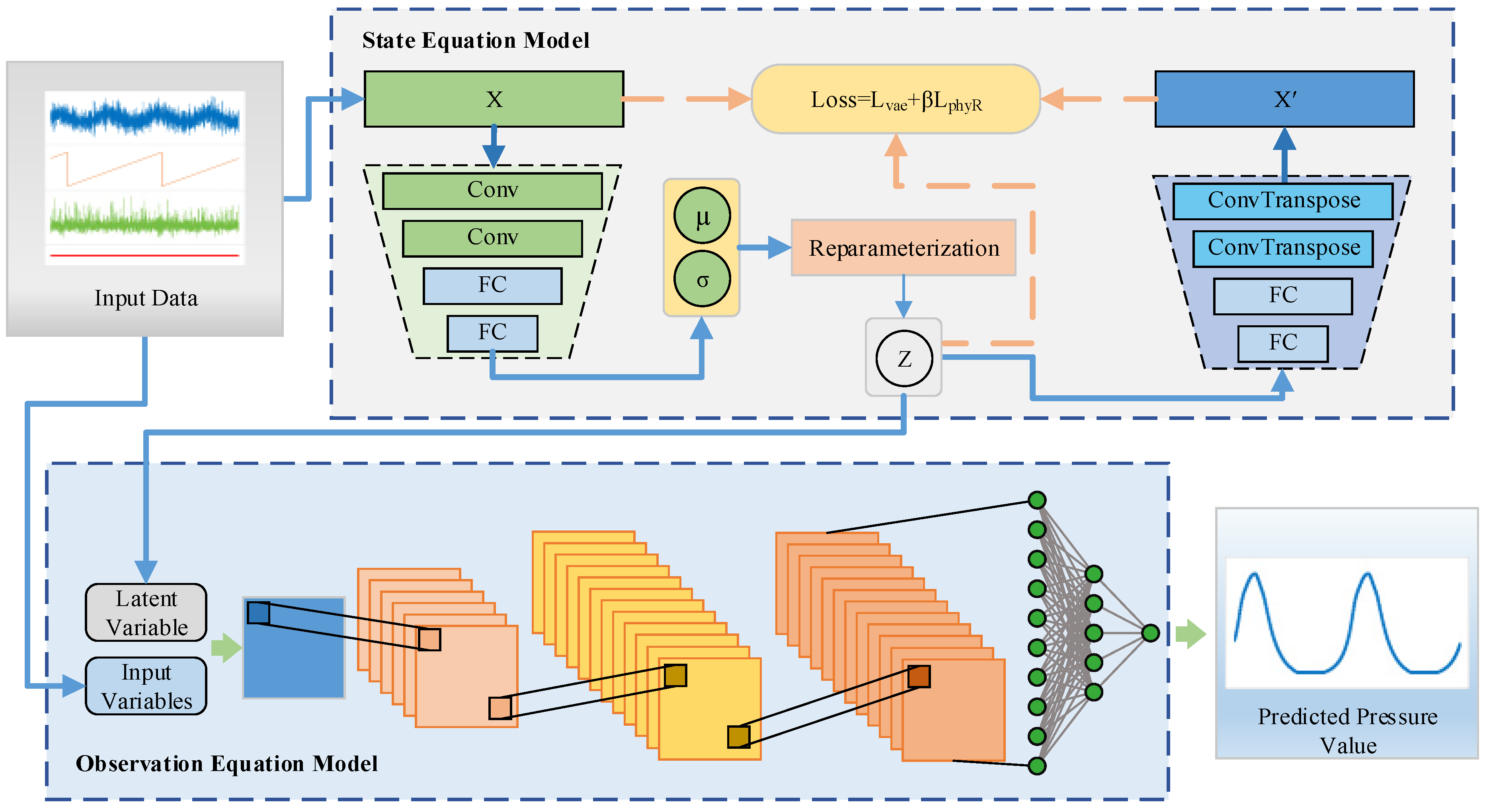
This paper proposes an adaptive prediction method for compressor cylinder dynamics based on a VAE-CNN-SSM. First, a VAE is employed to generate latent variables associated with valve motion states, thereby constructing the state equation. By embedding physical information of valve motion into the latent variable generation process, the model can effectively capture valve dynamics under complex leakage conditions. Subsequently, a CNN-based observation equation is developed to extract nonlinear features from latent variables, input variables, and pressure data, enabling high-precision prediction of cylinder pressure. The proposed method demonstrates excellent predictive performance in handling diverse leakage scenarios. The overall framework of this method is illustrated in Figure 3.

3.2. Dynamic System Based on State Space Model

When a valve leaks or changes operating conditions, the change in cylinder pressure becomes difficult to predict. Traditional methods make it difficult to accurately describe this complex dynamic relationship. The motion state of valves is often unobservable and cannot be directly obtained through simple sensors. With the increasing complexity of operating conditions, modeling and prediction tasks have become increasingly difficult. The State Space Model has significant advantages in dealing with such complex dynamic systems. SSM divides the dynamics of the system into two parts: the state equation and the observation equation. The state equation is used to describe how the internal state of a system evolves over time, while the observation equation describes the relationship between the observable variables of the system and the internal state. Therefore, this paper captures the dynamic changes of the valve by establishing a state equation, and then establishes an observation equation to infer the cylinder pressure from the valve motion state. It can accurately describe the dynamic behavior of the system under complex working conditions and achieve efficient prediction of cylinder pressure. Specifically, the state equation is used to describe the motion state of valves, where the valve opening is taken as the key state variable of valve motion, which can reflect the real-time dynamic information of the valve. The mathematical description of the equation of state is as follows:

$$h_t=A_{t-1}{h}_{t-1}+B_{t-1}{x}_{t-1}+{\omega }_t$$

(6)

where $h_t$ represents the hidden state vector at time t, which is the opening information of the valve. $x_t$ represents the input vector at time t, which represents the input vector of the system at that time, including input information such as intake pressure, intake temperature, crankshaft angle, and leakage size. $A_t$ is the state transition matrix used to describe the update rules of the state vector, and $B_t$ is the control input matrix used to describe the impact of the input vector on the valve state $h_t$. ${\omega }_t$ is the process noise, usually assumed to be Gaussian noise.

The observation equation describes how observable data can be generated from the system state. Using cylinder pressure as a key observation variable in the compressor system can reflect the overall operating status of the compressor. The mathematical expression of the observation equation is

$$y_t=C_t{h}_t+D_t{x}_t+{\upsilon }_t$$

(7)

where $y_t$ represents the observation vector at time t, which is the cylinder pressure. It can reflect the system’s response to external inputs and internal hidden states. $C_t$ is the observation matrix that describes how the valve opening $h_t$ is mapped to the cylinder pressure $y_t$. $D_t$ is a direct transfer matrix that describes the direct impact of input vectors on cylinder pressure. ${\mathrm{\upsilon }}_t$ is the observation noise, usually Gaussian noise, representing measurement error.

3.3. State Equation Model Based on VAE

In order to solve the state equation of the state space model, it is impossible to accurately determine the state transition matrix and control input matrix of the state equation because the valve opening variable is unobservable. A powerful generative model is needed to directly generate state variables to achieve the function of state equations. VAE is an autoencoder based on Bayesian variational inference. The ability to compress a high-dimensional random vector into latent variables in a low dimensional space through variational encoding [30]. It is different from traditional autoencoders that describe latent variables numerically. The model constructed based on VAE can obtain effective features for different operating conditions. It describes latent variables in a probabilistic manner, which provides more flexibility and robustness in describing the operating status of valves.

VAE mainly includes an encoder and a decoder. Firstly, the encoder is used to encode the input data, generating the mean $\mu$ and variance $\sigma$ of the latent variable $z$. Therefore, the latent variable $z$ is generated from the distribution of $p_{\theta }(z)$. The relevant process is

$$p_{\theta }\left(z|x\right)={\displaystyle \frac{p_{\theta }\left(x|z\right)p_{\theta }\left(z\right)}{p_{\theta }\left(x\right)}}$$

(8)

The decoder reconstructs the original input data $x\prime$ by mapping the distribution of the latent variable $z$. The specific process is as follows:

$$p_{\theta }(x\prime )=\int p_{\theta }(x\prime |z)p_{\theta }(z)dz$$

(9)

where $\mathrm{x}=\left\{x_1,x_2,\dots ,x_n\right\}$ represents the input dataset. $p_{\theta }(z|x)$ is the posterior distribution of the latent variable. However, since $z$ is unknown, it is difficult to directly calculate the posterior distribution $p_{\theta }(z|x)$ of $z$, so VAE uses Gaussian distribution $q_{\phi }(z|x)$ to approximate the true posterior distribution. $\theta$ and $\phi$ are the parameters of the model.

3.3.1. Loss Function Design

In order to ensure that the distributions of $p_{\theta }(z|x)$ and $q_{\phi }(z|x)$ are as similar as possible. VAE uses Kullback–Leibler (KL) divergence to identify the distance between $q_{\phi }(z|x)$ and the true posterior distribution $p_{\theta }(z|x)$ [31]. Therefore, the logarithmic likelihood of the dataset $\mathrm{x}$ can be expressed as

$${logp}_{\theta }\left(x\right)=D_{KL}(q_{\phi }(z|x)\Vert p_{\theta }\left(z|x\right))+{\mathcal{L}}_{vae}\left(\theta ,\phi ,x\right)$$

(10)

Since the KL distance is always non negative, ${logp}_{\theta }\left(x\right)\ge {\mathcal{L}}_{vae}(\theta ,\phi ,x)$. Maximizing the value of ${logp}_{\theta }\left(x\right)$ is equivalent to maximizing the lower limit ${\mathcal{L}}_{vae}(\theta ,\phi ,x)$. It can be expressed as

$${\mathcal{L}}_{vae}(\theta ,\phi ,x)=-D_{KL}(q_{\phi }(z|x)|{|p}_{\theta }\left(z\right))+E_{q_{\phi }\left(z|x\right)}\left(\mathit{log}\left(p_{\theta }\left(x|z\right)\right)\right)$$

(11)

The first term on the right-hand side of the above equation represents the regularization term, while the second term denotes the reconstruction error of the input data. Although the primary objective of a VAE is to reconstruct input data, the main purpose of introducing this structure in this paper is to generate latent variables that can characterize valve operating states, thereby assisting in the adaptive prediction of cylinder pressure. Since valve lift is difficult to measure directly, this paper infers the valve opening and closing states using acoustic emission (AE) signals and crank angle information. Specifically, AE signals collected during the valve opening and closing processes are correlated with simultaneously recorded crank angle data to determine the crank angle interval corresponding to valve opening. Based on this interval, the valve’s open or closed state can be identified at any given time, providing a reference value of valve lift for physical constraints. By incorporating the parameter of valve opening state $\alpha$ into the VAE loss function, a physical information error term is introduced to constrain the generated latent variables to approximate the valve lift reference. The formula is

$${\mathcal{L}}_{phyR}=\sqrt{{{\displaystyle \frac{1}{n}}\left(z-\alpha \right)}^2}$$

(12)

The loss function based on the VAE state equation is

$$\mathcal{L}\left(\theta ,\phi ;x\right)={\mathcal{L}}_{vae}+{\beta \mathcal{L}}_{phyR}$$

(13)

where $\beta$ is the adjustment coefficient.

3.3.2. VAE Structure

In order to calculate the gradient of the loss function, we need to sample $q_{\phi }(z|x)$. However, directly sampling latent variables from $q_{\phi }(z|x)$ would result in data being non differentiable. The reparameterization technique decomposes the sampling process into a deterministic transformation. The main process is to first introduce the ${ϵ}_i$ noise variable, which is obtained by sampling from the standard normal distribution, and then establishing the relationship between the latent variable $z$ and the noise ${ϵ}_i$. The formula is as follows:

$$z_i={\mu }_i+{\sigma }_i·{ϵ}_i$$

(14)

where ${\mu }_i$ is the mean of the latent variable distribution, and ${\sigma }_i$ is the variance of the distribution. The above function can convert the sampling process of latent variables into a deterministic function, allowing gradient backpropagation to optimize latent variable $z$.

In the VAE model presented in this paper, the encoder consists of two convolutional layers and two fully connected layers, while the decoder consists of two fully connected layers and a transposed convolutional layer. The specific structure is shown in Figure 4.

3.4. Observation Equation Model Based on CNN

In the adaptive prediction of reciprocating compressor cylinder dynamics, the traditional observation equation of the state-space model usually relies on prior physical models and accurate acquisition of model parameters. However, such models often fail to accurately describe complex nonlinear processes. Deep learning provides an effective alternative, as it can automatically learn nonlinear relationships and feature representations from data, thereby improving the estimation and prediction of cylinder dynamic characteristics. Convolutional Neural Network is a specialized class of deep neural networks [32], particularly effective in capturing local spatial and temporal correlations. In the case of compressor cylinder pressure prediction, valve leakage alters valve motion and introduces complex variations in pressure evolution. Through convolution operations, CNN can efficiently extract these features, model spatiotemporal changes, and capture nonlinear relationships. Therefore, this paper constructs a CNN-based observation equation to capture the dynamic variations of cylinders under different leakage conditions and to achieve accurate prediction of cylinder pressure.

The core of CNN is convolution operation, which reduces the number of parameters through local connections and shared weights, while preserving local features in the input data. In order to adapt to the prediction task of cylinder pressure, this paper designs a deep convolutional neural network structure. The model structure consists of multiple convolutional layers, pooling layers, and fully connected layers, which extract the complex spatiotemporal dependencies between valve leakage behavior and cylinder motion characteristics layer by layer. The specific structure is shown in Figure 5.

When processing data, the convolution operation of CNN can be expressed as

$$h_i^l=f\left(\sum _{i=1}^N{W}_i^l·X_i+b^l\right)$$

(15)

where $h_t^l$ represents the convolution output of the $l$ layer, $W_i^l$ is the convolution kernel, $X_i$ represents the input data, $b^l$ is the bias, and $f$(·) is the activation function. In this paper, $ReLU$ activation function is chosen. Through convolution operations, CNN can automatically learn and extract local features of input data, including the impact of valve leakage on cylinder pressure fluctuations.

The pooling operation is to further reduce the feature dimension. Adding a pooling layer after the convolutional layer can down sample the local features output by the convolutional layer, reduce data size, and enhance the model’s generalization ability. Generally, the max pooling layer is selected, and its formula can be expressed as

$$M_t^l=MaxPooling\left(h_i^l\right)$$

(16)

The output of the pooling layer needs to be further flattened and then connected to the fully connected layer to calculate the final pressure prediction value.

4. Experimental Details

4.1. Experimental Setup

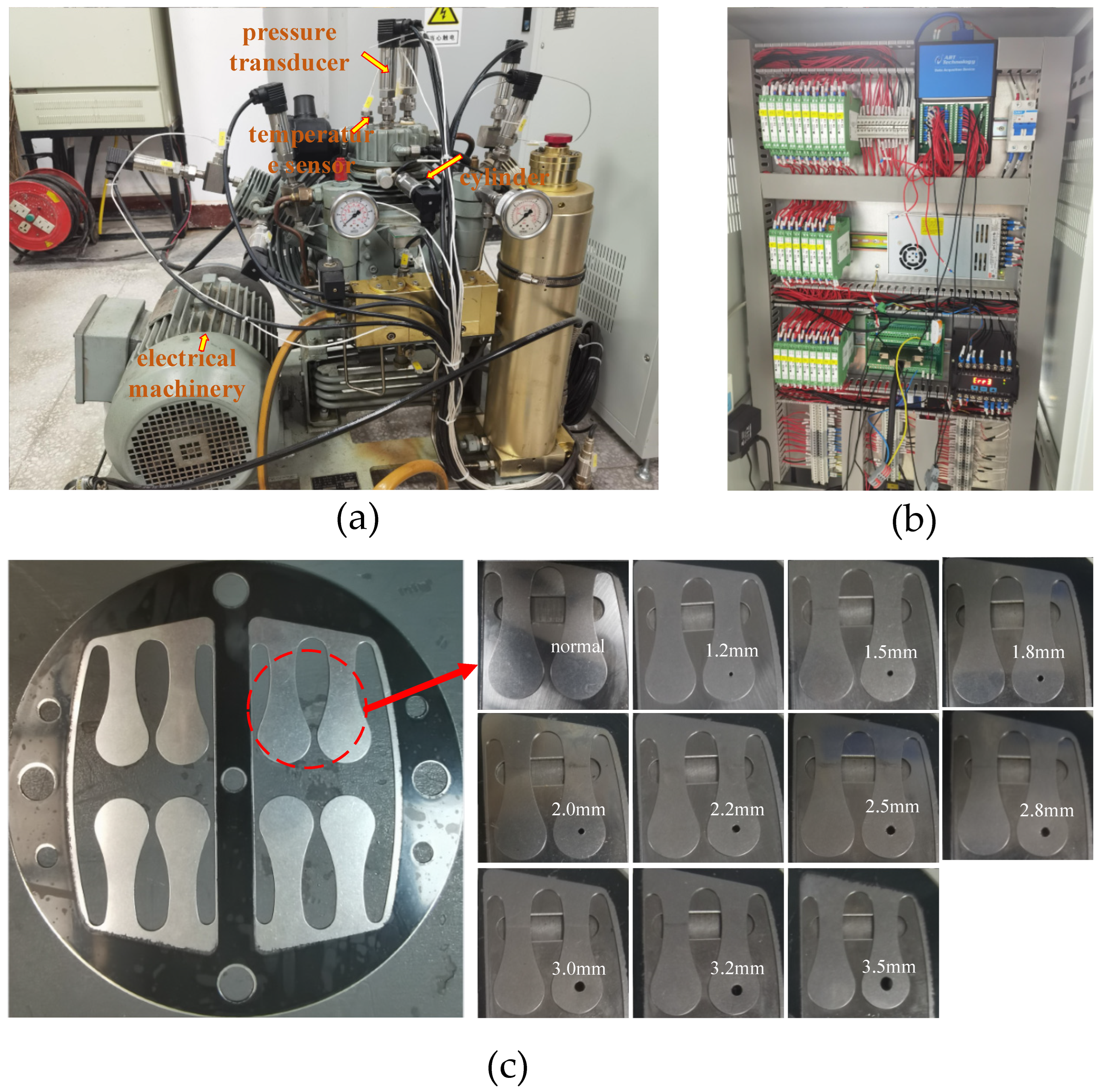
To verify the effectiveness of the proposed model, an experimental platform for reciprocating compressors was constructed. Sensors were installed on the compressor to measure cylinder temperature, pressure, and crankshaft speed. The cylinder pressure was measured using a JYB-KO-H (Beijing Kunlun Coast Sensing Technology Co., Ltd., Beijing, China) pressure sensor with a measurement range of 0–1.0 MPa and an accuracy of 0.1% of full scale(F.S.). The cylinder temperature was monitored by a JWB/PT100 (Beijing Kunlun Coast Sensing Technology Co., Ltd., Beijing, China) thermocouple with a measurement range of −50 to 300 °C and an accuracy of 0.2% F.S. The crankshaft angle and rotational speed were recorded by an E6B2-CWZ6C encoder (Omron Automation (China) Co., Ltd., Shanghai, China) with a resolution of 2500 pulses per revolution. To simulate different valve leakage conditions, circular holes with various diameters were machined into the reed valve. In this paper, eleven hole sizes were selected based on the reed valve dimensions to represent leakage scenarios, namely 1.2 mm, 1.5 mm, 1.8 mm, 2.0 mm, 2.2 mm, 2.5 mm, 2.8 mm, 3.0 mm, 3.2 mm, and 3.5 mm. Data under these different leakage conditions were collected for model validation. The experimental platform and the processed reed valves are illustrated in Figure 6.

4.2. Model Parameter Settings

To verify the effectiveness and superiority of the proposed model in this paper. This paper compares and analyzes popular time series prediction algorithms such as XGBOOST, MLP, RNN, LSTM, and CNN, and adjusts various model parameters to achieve optimal performance. The specific model parameters are shown in

Table 1. Parameters of each model.

Model	Parameters
XGBOOST	Max_depth = 5, colsample_bytree = 0.3, learning_rate = 0.1, alpha = 10, n_estimators = 100
MLP	Neuron = 64, epoch = 500, loss function = MSE, learning rate = 0.01, activation function is ReLU
RNN	Neuron = 64, epoch = 500, loss function = MSE, learning rate = 0.01, activation function is ReLU
LSTM	Neuron = 64, epoch = 500, loss function = MSE, learning rate = 0.01, activation function is ReLU
CNN	Neuron = 32, epoch = 500, loss function = MSE, learning rate = 0.01, activation function ReLU, convolution kernel 3 × 3
Proposed Method	Neuron = 32, epoch = 500, loss function = MSE, learning rate = 0.01, activation function ReLU, convolution kernel 3 × 3

. All model training mentioned in this paper was conducted under the conditions of Windows 11 operating system, NVIDIA 4080 graphics card, and Intel Core i9 14900KF processor.

4.3. Evaluation Indicators

In order to effectively evaluate the performance of various models, this experiment considers three evaluation indicators: mean error (MAE), root mean square error (RMSE) and coefficient of determination (R2) to evaluate the performance of different methods. MAE can more intuitively represent the size of the model’s prediction error. RMSE can better measure the deviation between predicted values and actual values. R2 can better evaluate the fitting degree of the overall prediction results.

$$MAE={\displaystyle \frac{1}{N}}{\sum }_{i=1}^N\left|y_i-{\widehat{y}}_i\right|$$

(17)

$$RMSE=\sqrt{{\displaystyle \frac{1}{N}}{\sum }_{i=1}^N{(y_i-{\widehat{y}}_i)}^2}$$

(18)

$$R^2=1-{\displaystyle \frac{{\sum }_{i=1}^N{\left(y_i-{\widehat{y}}_i\right)}^2}{{\sum }_{i=1}^N{\left(y_i-{\overline{y}}_i\right)}^2}}$$

(19)

where ${\widehat{y}}_i$ is the predicted cylinder pressure value, $y_i$ is the actual cylinder pressure value, ${\overline{y}}_i$ is the average actual cylinder pressure value, and $N$ is the sample size.

5. Results Analysis

In order to analyze and compare the predictive performance of different models, this section conducts experiments and evaluations on the prediction accuracy, generalization, and ablation study of the proposed model. The following are the details related to the predicted results.

5.1. Prediction Accuracy Evaluation

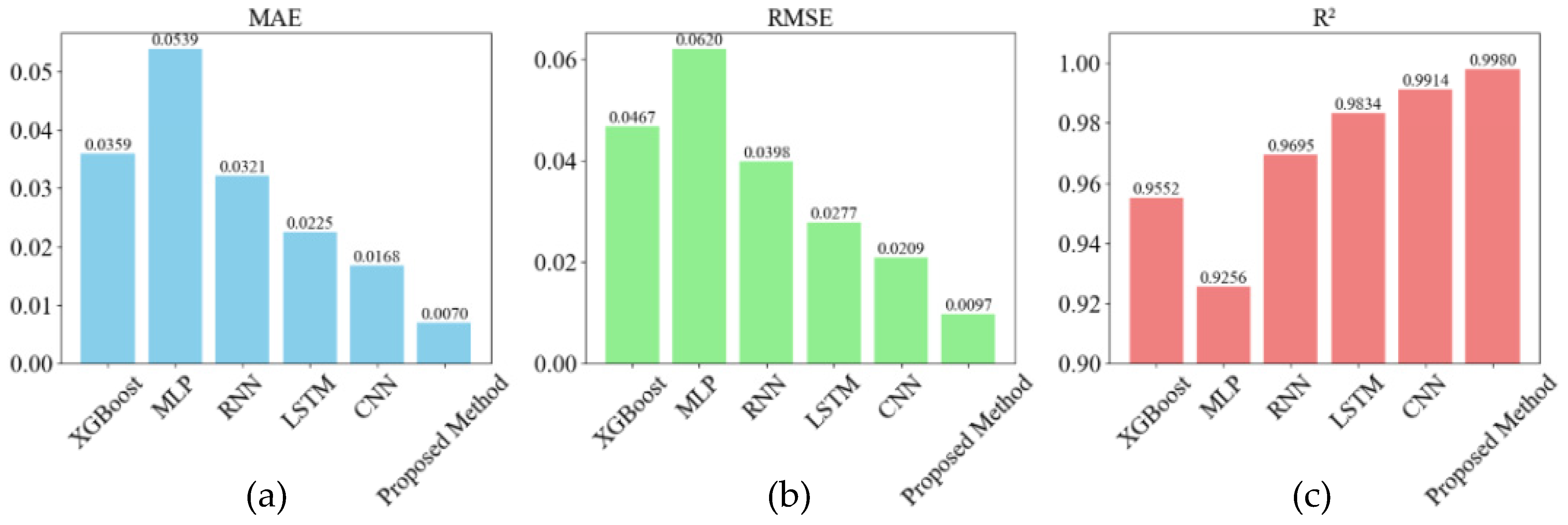
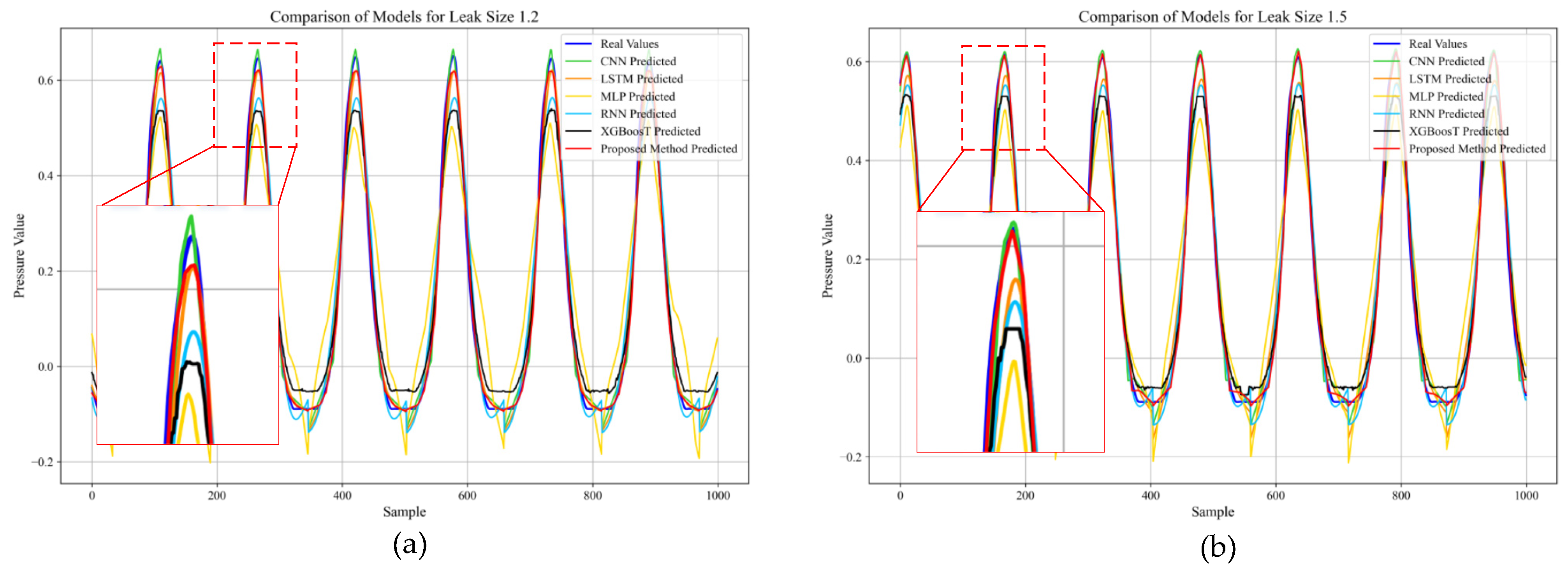
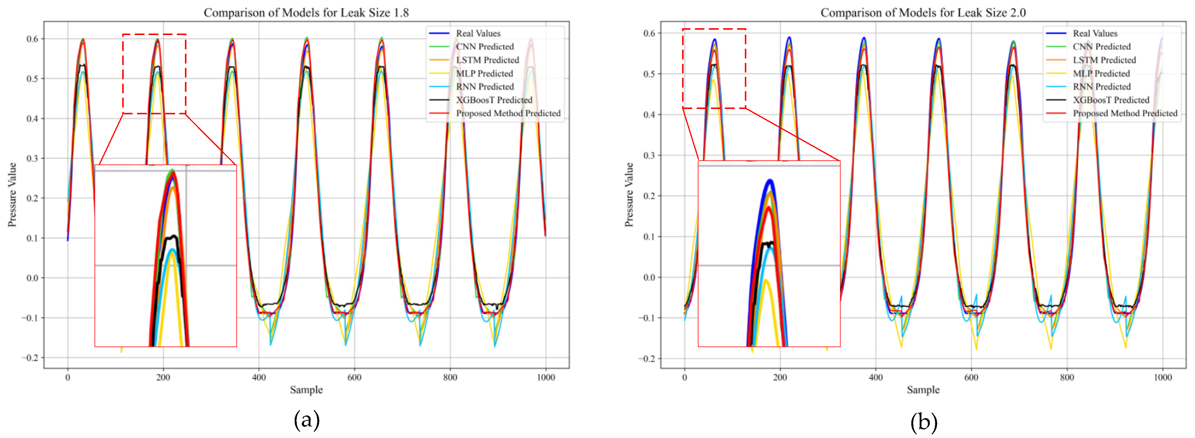
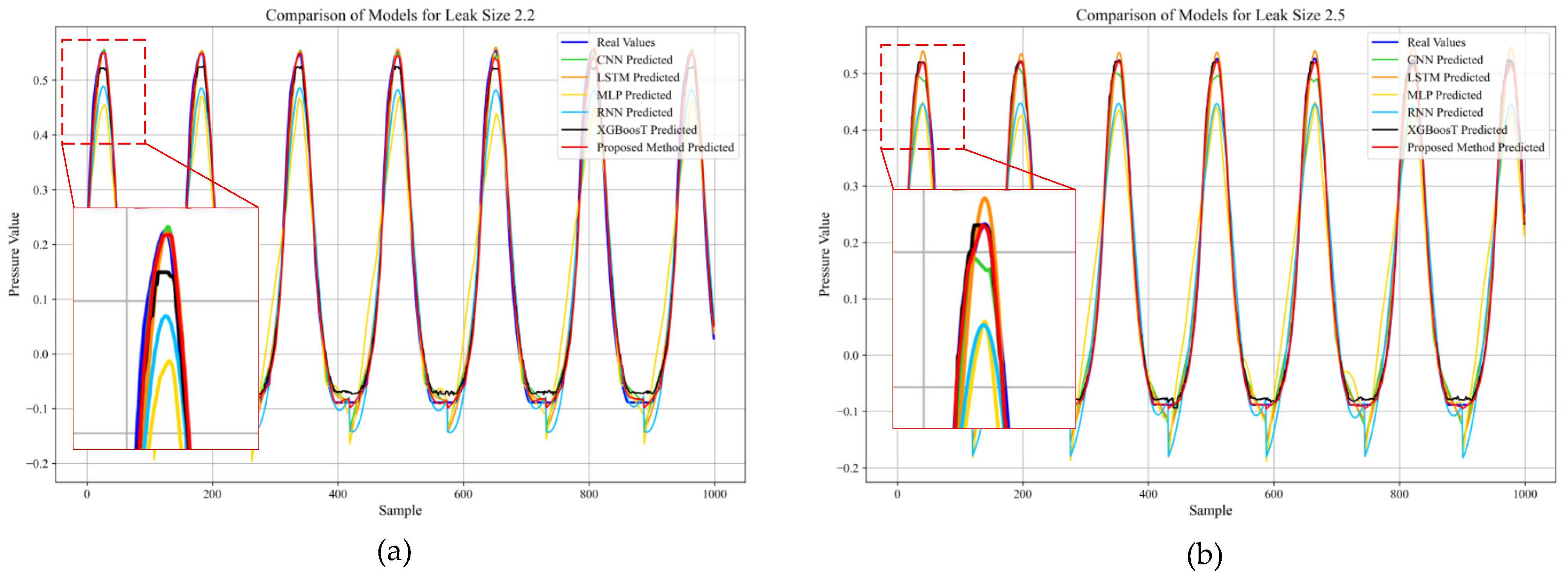
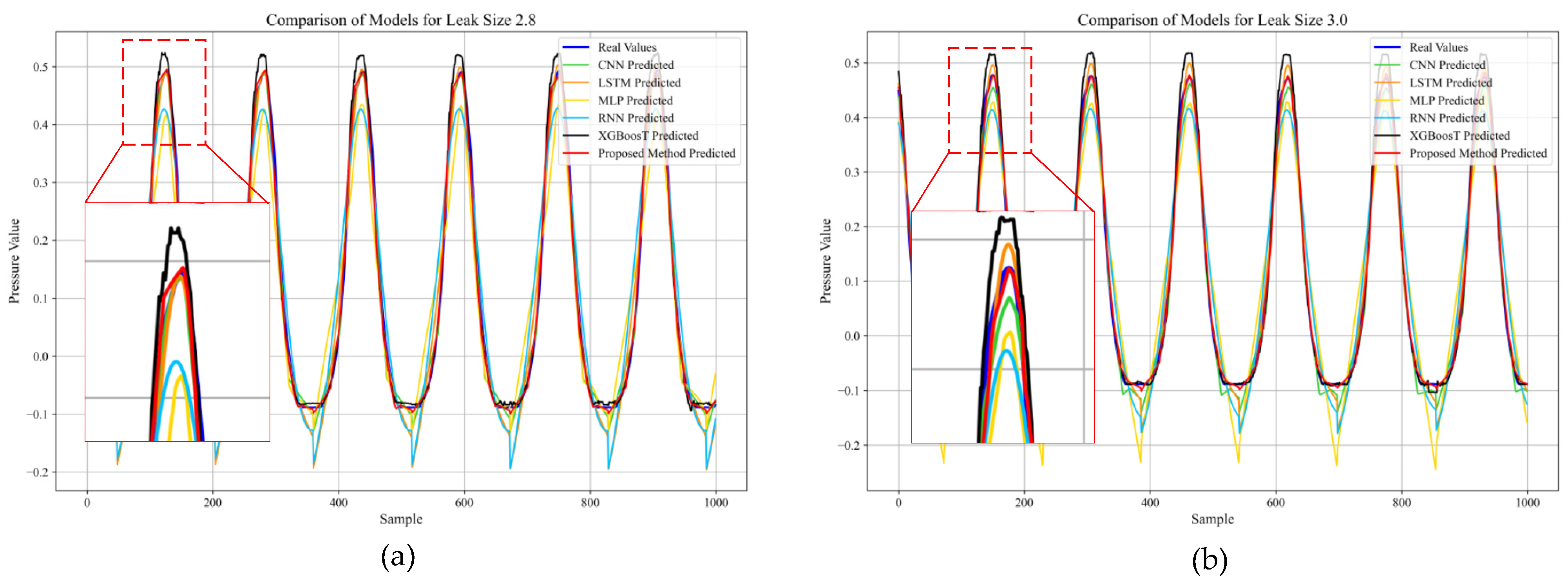
In order to evaluate the prediction accuracy of different models, this paper conducts cylinder pressure training and prediction for various leakage situations on six models. The prediction results of each model are shown in

Table 2. Comparison of six models’ predictive performance indicators.

Leakage Size		0	1.2	1.5	1.8	2	2.2	2.5	2.8	3	3.2	3.5
XGBOOST	MAE	0.0638	0.0543	0.0477	0.0491	0.0409	0.0319	0.0261	0.0237	0.0140	0.0159	0.0273
	RMSE	0.0788	0.0660	0.0571	0.0830	0.0487	0.0377	0.0303	0.0284	0.0282	0.0193	0.0360
	R2	0.9159	0.9355	0.9483	0.8814	0.9596	0.9735	0.9813	0.9819	0.9811	0.9906	0.9578
MLP	MAE	0.0781	0.0632	0.0541	0.0505	0.0563	0.0511	0.0514	0.0463	0.0491	0.0511	0.0421
	RMSE	0.0893	0.0705	0.0601	0.0571	0.0652	0.0586	0.0600	0.0557	0.0571	0.0590	0.0499
	R2	0.8891	0.9249	0.9440	0.9456	0.9279	0.9381	0.9294	0.9284	0.9216	0.9149	0.9182
RNN	MAE	0.0481	0.0411	0.0383	0.0348	0.0359	0.0319	0.0266	0.0233	0.0227	0.0214	0.0288
	RMSE	0.0616	0.0505	0.0469	0.0432	0.0448	0.0390	0.0330	0.0311	0.0271	0.0261	0.0346
	R2	0.9468	0.9612	0.9658	0.9689	0.9658	0.9726	0.9787	0.9779	0.9824	0.9833	0.9607
LSTM	MAE	0.0326	0.0279	0.0250	0.0197	0.0223	0.0199	0.0164	0.0193	0.0174	0.0176	0.0289
	RMSE	0.0393	0.0323	0.0296	0.0233	0.0262	0.0256	0.0201	0.0242	0.0217	0.0226	0.0403
	R2	0.9784	0.9841	0.9864	0.9909	0.9883	0.9882	0.9920	0.9867	0.9887	0.9875	0.9465
CNN	MAE	0.0197	0.0191	0.0185	0.0161	0.0170	0.0180	0.0130	0.0162	0.0158	0.0142	0.0173
	RMSE	0.0246	0.0230	0.0230	0.0196	0.0206	0.0228	0.0168	0.0196	0.0202	0.0180	0.0214
	R2	0.9915	0.9919	0.9918	0.9936	0.9928	0.9906	0.9944	0.9913	0.9902	0.9921	0.9850
Proposed Method	MAE	0.0066	0.0053	0.0068	0.0062	0.0073	0.0098	0.0044	0.0087	0.0084	0.0058	0.0076
	RMSE	0.0098	0.0075	0.0093	0.0086	0.0100	0.0127	0.0059	0.0120	0.0112	0.0082	0.0114
	R2	0.9986	0.9991	0.9986	0.9988	0.9983	0.9971	0.9993	0.9967	0.9970	0.9984	0.9957

and Figure 7.

Table 2 shows the detailed prediction results of 11 leakage scenarios. In order to facilitate the comparison of model prediction accuracy, the mean bar chart of the 11 results is plotted as shown in Figure 8. From Figure 8, it can be obtained that the average MAE, RMSE, and R² of XGBOOST’s prediction indicators are 0.0359, 0.0467, and 0.9552, respectively. XGBOOST relies on its powerful tree structure to handle non-linear relationships between features and has good prediction accuracy. However, when the leakage situation becomes complex, XGBOOST is unable to cope with complex multi working conditions and is prone to losing stability and accuracy.

Figure 8 shows that the average MAE of MLP is 0.0539, the average RMSE is 0.0620, and the average R² is 0.9256. MLP is a basic neural network model with certain nonlinear fitting ability, but it is difficult to capture the characteristics of dynamic changes in complex working conditions, and its ability to predict pressure under different leakage situations is insufficient.

The average MAE of RNN is 0.0321, the average RMSE is 0.0398, and the R² is 0.9695. RNN can capture certain historical information and reflect it in prediction, demonstrating superior ability compared to certain time series models. However, in long-term complex leakage scenarios, it is easily limited by the vanishing gradient problem, leading to a decrease in the ability to predict long-term changes.

The average MAE of LSTM is 0.0225, the average RMSE is 0.0277 and the average R² is 0.9834. In complex leakage situations, LSTM can capture long-term and short-term changes well, demonstrating strong time series modeling capabilities. However, it may encounter overfitting and limited predictive ability in complex state changes.

The average MAE of CNN is 0.0168, the average RMSE is 0.0209, and the average R² is 0.9914. CNN is good at extracting information from local features and spatial relationships, and has certain advantages in smoothing and feature extraction of time series data. However, its performance is limited in dynamic modeling with long-term dependencies, making it difficult to directly cope with complex state changes.

The average MAE of the model prediction results proposed in this paper is 0.0070, the average RMSE is 0.0097, and the average R² is 0.9980. The three evaluation indicators of the model are all the best among the six models. This model can cope with various leakage conditions by generating latent variables through VAE combined with physical information. The CNN-based observation equation in the model extracts local features to accurately describe the dynamic state of the cylinder, ultimately achieving accurate prediction of cylinder pressure under different leakage conditions.

5.2. Generalization Evaluation

In order to analyze the generalization of different models, this paper adopts a specific dataset extrapolation testing strategy. Specifically, a dataset of individual operating conditions will be extracted in order so that they do not participate in model training, and then this dataset will be used for cylinder pressure prediction to observe the model’s generalization ability. The following are the prediction results of six models under this testing method.

The results from Figure 8, Figure 9, Figure 10, Figure 11, Figure 12 and Figure 13 show that XGBOOST, as a tree-based model, mainly relies on existing dataset features for predicting unseen datasets. When there is a significant change in the leakage condition, XGBOOST finds it difficult to adapt to the dynamic characteristics of the new dataset, resulting in large prediction errors and insufficient generalization ability. The utilization of time information by MLP is limited, and it is difficult for MLP to capture dynamic changes when facing unseen working conditions. Therefore, the model has poor generalization ability. Due to the vanishing gradient problem and its insufficient modeling of long-term states, RNN cannot effectively predict unseen datasets. Although LSTM exhibits strong generalization ability, it may be affected by model complexity and computational cost, which can affect the accuracy of predictions. Due to the fact that CNN mainly focuses on local features and lacks adaptability to long-term and complex operating conditions, it is prone to significant errors when generalizing to significantly changing leakage conditions. The model proposed in this paper can capture the motion information of valves through latent variables generated by VAE, and based on the CNN’s ability to extract local features, the model exhibits strong generalization in datasets without observed operating conditions. Therefore, even in the event of new leakage changes, the model can still effectively capture its effective features, thereby achieving accurate prediction.

5.3. Ablation Study

To verify the necessity of each component in the proposed model, this paper analyzes three variants of the model. The first variant model is VAE-CNN-SSM without physical properties, which is used to verify the impact of physical information on the generation of latent variables and thus on the prediction accuracy of the model. The second variant model is VAE-BP-SSM, which replaces CNN with a regular neural network to analyze the impact of adding CNN on the model’s feature extraction ability. The third variant model is a standalone CNN, which is used to analyze the impact of latent variables generated by VAE on prediction accuracy. The following are the prediction results of various variant models.

From the results in

Table 3. Comparison of Prediction Performance Indicators of Various Variant Models.

Leakage Size		0	1.2	1.5	1.8	2	2.2	2.5	2.8	3	3.2	3.5	Average
MAE	Proposed Method	0.0066	0.0053	0.0068	0.0062	0.0073	0.0098	0.0044	0.0087	0.0084	0.0058	0.0076	0.0070
	VAECNNSSM	0.0183	0.0155	0.0149	0.0139	0.0151	0.0156	0.0129	0.0157	0.0147	0.0135	0.0164	0.0151
	VAEBPSSM	0.0175	0.0143	0.0140	0.0131	0.0160	0.0166	0.0165	0.0219	0.0190	0.0206	0.0220	0.0174
	CNN	0.0197	0.0191	0.0185	0.0161	0.0170	0.0180	0.0130	0.0162	0.0158	0.0142	0.0173	0.0168
RMSE	Proposed Method	0.0098	0.0075	0.0093	0.0086	0.0100	0.0127	0.0059	0.0120	0.0112	0.0082	0.0114	0.0097
	VAECNNSSM	0.0222	0.0187	0.0187	0.0168	0.0175	0.0194	0.0158	0.0198	0.0180	0.0163	0.0203	0.0185
	VAEBPSSM	0.0207	0.0183	0.0185	0.0157	0.0189	0.0200	0.0189	0.0259	0.0216	0.0232	0.0254	0.0206
	CNN	0.0246	0.0230	0.0230	0.0196	0.0206	0.0228	0.0168	0.0196	0.0202	0.0180	0.0214	0.0209
R2	Proposed Method	0.9986	0.9991	0.9986	0.9988	0.9983	0.9971	0.9993	0.9967	0.9970	0.9984	0.9957	0.9980
	VAECNNSSM	0.9931	0.9946	0.9946	0.9953	0.9948	0.9932	0.9951	0.9910	0.9922	0.9935	0.9865	0.9931
	VAEBPSSM	0.9940	0.9949	0.9947	0.9959	0.9939	0.9928	0.9930	0.9847	0.9888	0.9868	0.9788	0.9908
	CNN	0.9915	0.9919	0.9918	0.9936	0.9928	0.9906	0.9944	0.9913	0.9902	0.9921	0.9850	0.9914

, it can be seen that the average MAE, RMSE, and R² of the VAE-CNN-SSM model without physical information are 0.0151, 0.0185, and 0.9931, respectively, indicating a significant decrease in performance compared to the model proposed in this paper. This indicates that adding physical information to the model proposed in this paper enables the latent variables generated by VAE to help the model identify features of different leakage situations. Adding physical information not only improves the interpretability of the model, but also enhances its prediction accuracy. VAE-BP-SSM has lower prediction accuracy. The average MAE is 0.0174, RMSE is 0.0206, and R2 is 0.9908. This indicates that adding CNN is necessary to enhance the ability to extract data features. Simple neural networks are unable to extract effective information from latent variables, which affects the predictive ability of the model. The prediction results of the standalone CNN model show an average MAE of 0.0168, RMSE of 0.0209, and R² of 0.9914. Due to the lack of latent variables and insufficient information on the leakage situation, the final prediction accuracy is low. Therefore, the experimental results of these three variant models demonstrate the feasibility and effectiveness of the proposed model in this paper.

6. Conclusions

This paper proposes a physics-guided VAE-CNN-SSM for adaptive prediction of compressor cylinder pressure under valve leakage failure. By embedding physical information into the VAE to generate latent variables, the model effectively captures valve motion states. Leveraging the feature extraction capability of CNN and the dynamic representation ability of the state-space model, the proposed framework achieves accurate prediction of cylinder pressure dynamics under valve leakage failure conditions. Comparative experiments with XGBoost, MLP, RNN, LSTM, and CNN demonstrate that the proposed method outperforms conventional approaches, achieving an average MAE of 0.0070, an average RMSE of 0.0097, and an average R² of 0.9980, which highlights its superior prediction accuracy and generalization capability. At the same time, ablation studies verify the effectiveness of each component of the proposed model. By integrating physical information with data-driven techniques, the model provides reliable prediction performance across different valve leakage failure conditions. However, the designed model is relatively complex and requires higher computational cost during training. Future work will focus on developing a lightweight version to reduce training cost while maintaining high prediction accuracy. In addition, factors such as valve wear, vibration, and temperature variation will be considered to enhance model robustness and applicability in industrial-scale compressor systems.

References

1. Zhou, W.; Su, H.; Liu, H.; Zhang, Y.; Qiu, N.; Gao, B. Leakage and Rotordynamic Performance of a Semi-Y Labyrinth Seal Structure for Centrifugal Pump Based on Multifrequency Whirl Method. J. Eng. Gas Turbines Power 2025, 147, 101022. [Google Scholar] [CrossRef]
2. Cui, W.; Wang, D.; Hong, X.; Liu, D.; Cao, X. Automated multi-functional system for the characterization of plate valves in reciprocating compressors. Instrum. Sci. Technol. 2024, 52, 494–515. [Google Scholar] [CrossRef]
3. Mu, G.; Wang, F.; Mi, X.; Gao, G. Dynamic modeling and analysis of compressor reed valve based on movement characteristics. Appl. Therm. Eng. 2019, 150, 522–531. [Google Scholar] [CrossRef]
4. Rigola, J.; Pérez-Segarra, C.D.; Oliva, A. Parametric studies on hermetic reciprocating compressors. Int. J. Refrig. 2005, 28, 253–266. [Google Scholar] [CrossRef]
5. Govindan, N.; Jayaraman, V.; Venkatasamy, R.; Ramasamy, M. Mathematical modeling and simulation of a reed valve reciprocating air compressor. Therm. Sci. 2009, 13, 47–58. [Google Scholar] [CrossRef]
6. Farzaneh-Gord, M.; Khoshnazar, H. Valve fault detection for single-stage reciprocating compressors. J. Nat. Gas Sci. Eng. 2016, 35, 1239–1248. [Google Scholar] [CrossRef]
7. Silva, L.R.; Deschamps, C.J. Modeling of gas leakage through compressor valves. Int. J. Refrig. 2015, 53, 195–205. [Google Scholar] [CrossRef]
8. Elhaj, M.; Gu, F.; Ball, A.D.; Albarbar, A.; Al-Qattan, M.; Naid, A. Numerical simulation and experimental study of a two-stage reciprocating compressor for condition monitoring. Mech. Syst. Signal Process. 2008, 22, 374–389. [Google Scholar] [CrossRef]
9. Damle, R.; Rigola, J.; Pérez-Segarra, C.D.; Castro, J.; Oliva, A. Object-oriented simulation of reciprocating compressors: Numerical verification and experimental comparison. Int. J. Refrig. 2011, 34, 1989–1998. [Google Scholar] [CrossRef]
10. Wang, Y.; Wang, J.; He, Z.; Sun, J.; Wang, T.; Liu, C. Investigation on Dynamic Characteristics of the Reed Valve in Compressors Based on Fluid-Structure Interaction Method. Appl. Sci. 2021, 11, 3946. [Google Scholar] [CrossRef]
11. Hwang, I.S.; Park, S.J.; Oh, W.; Lee, Y.L. Linear compressor discharge valve behavior using a rigid body valve model and a FSI valve model. Int. J. Refrig. 2017, 82, 509–519. [Google Scholar] [CrossRef]
12. Zhao, B.; Jia, X.; Sun, S.; Wen, J.; Peng, X. FSI model of valve motion and pressure pulsation for investigating thermodynamic process and internal flow inside a reciprocating compressor. Appl. Therm. Eng. 2018, 131, 998–1007. [Google Scholar] [CrossRef]
13. Tao, W.; Guo, Y.; He, Z.; Peng, X. Investigation on the delayed closure of the suction valve in the refrigerator compressor by FSI modeling. Int. J. Refrig. 2018, 91, 111–121. [Google Scholar] [CrossRef]
14. Wu, W.; Guo, T.; Peng, C.; Li, X.; Li, X.; Zhang, Z.; Xu, L.; He, Z. FSI simulation of the suction valve on the piston for reciprocating compressors. Int. J. Refrig. 2022, 137, 14–21. [Google Scholar] [CrossRef]
15. Bacak, A.; Pınarbaşı, A.; Dalkılıç, A.S. A 3-D FSI simulation for the performance prediction and valve dynamic analysis of a hermetic reciprocating compressor. Int. J. Refrig. 2023, 150, 135–148. [Google Scholar] [CrossRef]
16. Fu, J.; Zhang, G.; Sun, X.; He, T.; Li, H. A combinatorial prediction model for the performance of fuel cell air compressor with air bearings considering accelerated decay characteristics. Appl. Therm. Eng. 2024, 253, 123784. [Google Scholar] [CrossRef]
17. Belman-Flores, J.M.; Ledesma, S.; Barroso-Maldonado, J.M.; Navarro-Esbrí, J. A comparison between the modeling of a reciprocating compressor using artificial neural network and physical model. Int. J. Refrig. 2015, 59, 144–156. [Google Scholar] [CrossRef]
18. Ledesma, S.; Belman-Flores, J.M.; Barroso-Maldonado, J.M. Analysis and modeling of a variable speed reciprocating compressor using ANN. Int. J. Refrig. 2015, 59, 190–197. [Google Scholar] [CrossRef]
19. Kumar, A.; Patil, S.; Kovacevic, A.; Ponnusami, S.A. Performance prediction and Bayesian optimization of screw compressors using Gaussian Process Regression. Eng. Appl. Artif. Intell. 2024, 133, 108270. [Google Scholar] [CrossRef]
20. Ghorbanian, K.; Gholamrezaei, M. An artificial neural network approach to compressor performance prediction. Appl. Energy 2009, 86, 1210–1221. [Google Scholar] [CrossRef]
21. Wang, Y.; Du, Q.; Li, Y.; Zhang, D.; Xie, Y. Field reconstruction and off-design performance prediction of turbomachinery in energy systems based on deep learning techniques. Energy 2022, 238, 121825. [Google Scholar] [CrossRef]
22. Li, H.; Zhou, S.; Kan, H.; Cong, M. Milling cutter condition reliability prediction based on state space model. J. Vibroengineering 2016, 18, 4312–4328. [Google Scholar] [CrossRef]
23. Pedregal, D.J.; Carmen Carnero, M. State space models for condition monitoring: A case study. Reliab. Eng. Syst. Saf. 2006, 91, 171–180. [Google Scholar] [CrossRef]
24. Zhang, Y.; Zhang, L. Intelligent fault detection of reciprocating compressor using a novel discrete state space. Mech. Syst. Signal Process. 2022, 169, 108583. [Google Scholar] [CrossRef]
25. Yao, Y.; Wang, W.; Huang, M. A state-space dynamic model for vapor compression refrigeration system based on moving-boundary formulation. Int. J. Refrig. 2015, 60, 174–189. [Google Scholar] [CrossRef]
26. Skordilis, E.; Moghaddass, R. A Double Hybrid State-Space Model for Real-Time Sensor-Driven Monitoring of Deteriorating Systems. IEEE Trans. Autom. Sci. Eng. 2020, 17, 72–87. [Google Scholar] [CrossRef]
27. Liu, H.T.; Liu, C.J.; Jiang, X.M.; Chen, X.; Yang, S.; Wang, X. Deep probabilistic time series forecasting using augmented recurrent input for dynamic systems. Mech. Syst. Signal Process. 2022, 177, 16. [Google Scholar] [CrossRef]
28. Zhou, H.; Wang, B.; Zio, E.; Wen, G.; Liu, Z.; Su, Y.; Chen, X. Hybrid system response model for condition monitoring of bearings under time-varying operating conditions. Reliab. Eng. Syst. Saf. 2023, 239, 109528. [Google Scholar] [CrossRef]
29. Liu, Y.; Li, Q.; Wang, K. Revealing the degradation patterns of lithium-ion batteries from impedance spectroscopy using variational auto-encoders. Energy Storage Mater. 2024, 69, 103394. [Google Scholar] [CrossRef]
30. Jing, T.; Zheng, P.; Xia, L.; Liu, T. Transformer-based hierarchical latent space VAE for interpretable remaining useful life prediction. Adv. Eng. Inform. 2022, 54, 101781. [Google Scholar] [CrossRef]
31. Mou, M.; Zhao, X.; Liu, K.; Hui, Y. Variational autoencoder based on distributional semantic embedding and cross-modal reconstruction for generalized zero-shot fault diagnosis of industrial processes. Process Saf. Environ. Prot. 2023, 177, 1154–1167. [Google Scholar] [CrossRef]
32. Guo, F.Y.; Zhang, Y.C.; Wang, Y.; Wang, P.; Ren, P.-J.; Guo, R.; Wang, X.-Y. Fault Detection of Reciprocating Compressor Valve Based on One-Dimensional Convolutional Neural Network. Math. Probl. Eng. 2020, 2020, 10. [Google Scholar] [CrossRef]
Figure 1. Structure of the valve and schematic diagram of the leakage. (a) valve open; (b) valve closed.
Actuators 14 00535 g001
Figure 2. The schematic diagram of pressure changes caused by valve leakage.
Actuators 14 00535 g002
Figure 3. VAE-CNN-SSM model framework diagram.
Actuators 14 00535 g003
Figure 4. Structure diagram based on VAE state equation model.
Actuators 14 00535 g004
Figure 5. Structure diagram based on CNN observation model.
Actuators 14 00535 g005
Figure 6. Experimental setup. (a) Compressor test bench; (b) Data collection device; (c) Valve fault simulation setting.
Actuators 14 00535 g006
Figure 7. Comparison of Average Prediction Indicators of Various Models. (a) MAE; (b) RMSE; (c) R2.
Actuators 14 00535 g007
Figure 8. Prediction Results of Models with Leakage Sizes of 1.2 and 1.5. (a) Leakage Sizes 1.2; (b) Leakage Sizes 1.5.
Actuators 14 00535 g008
Figure 9. Prediction Results of Models with Leakage Sizes of 1.8 and 2.0. (a) Leakage Sizes 1.8; (b) Leakage Sizes 2.0.
Actuators 14 00535 g009
Figure 10. Prediction Results of Models with Leakage Sizes of 2.2 and 2.5. (a) Leakage Sizes 2.2; (b) Leakage Sizes 2.5.
Actuators 14 00535 g010
Figure 11. Prediction Results of Models with Leakage Sizes of 2.8 and 3.0. (a) Leakage Sizes 2.8; (b) Leakage Sizes 3.0.
Actuators 14 00535 g011
Figure 12. Prediction Results of Models with Leakage Sizes of 3.2 and 3.5. (a) Leakage Sizes 3.2; (b) Leakage Sizes 3.5.
Actuators 14 00535 g012
Figure 13. Comparison of Average Prediction Indicators under Extrapolation Strategy. (a) MAE; (b) RMSE; (c) R2.
Actuators 14 00535 g013