A Study on Compensation for Operating Region Variations in an In-Wheel PMSM Under Temperature Changes Using Neural Network Algorithms

Abstract

This study proposes a compensation method for operating region variations in in-wheel PMSMs, which are widely used in small mobility applications such as e-scooters and e-bikes. As motor temperature increases during operation, electrical parameters such as inductance vary, leading to unstable control. To address this, a Single-Layer Backpropagation Neural Network (SLBPNN) is used to estimate inductance variations in real-time. The proposed algorithm adjusts the motor’s operating point to maintain stable performance under thermal stress. Simulation results using MATLAB 2024b confirm the model’s effectiveness by estimating inductance from voltage, current, speed, and position inputs. Experimental validation further demonstrates that the proposed method compensates for the shift in the operating region due to temperature changes, improving the overall motor efficiency.

1. Introduction

Permanent Magnet Synchronous Motors (PMSMs) have emerged as a prominent choice in modern electromechanical systems, driven by their superior efficiency, high torque density, and precise controllability compared to conventional motor types such as induction machines. The rapid advancement of high-energy rare-earth permanent magnets, coupled with progress in power electronics, digital control hardware, and sophisticated control strategies (e.g., Field-Oriented Control), has accelerated their integration into a wide range of applications, including electric vehicles, industrial automation, robotics, and renewable energy conversion systems. PMSMs inherently exhibit lower rotor losses, reduced thermal stress, and higher dynamic responsiveness, enabling enhanced energy efficiency and extended operational lifespan [1]. In the context of global energy conservation initiatives and carbon emission reduction targets, Permanent magnet synchronous motors constitute a key enabling technology for sustainable mobility and advanced high-performance motion control applications [2]. Consequently, ongoing research focuses on further improving their control accuracy, fault tolerance, and cost-effectiveness to expand their applicability in future-generation electrified systems. In addition to their high efficiency and widespread industrial adoption, PMSMs are subject to inherent parameter variations under changing environmental conditions, particularly temperature fluctuations [3]. Variations in key electrical parameters—such as the d-axis and q-axis inductances ($L_d,L_q$) and stator resistance ($R_s$)—can significantly alter the motor’s operational characteristics [4,5]. For instance, an increase in stator resistance due to copper heating leads to higher copper losses and reduced torque production efficiency, while temperature-dependent changes in $L_d$ and $L_q$ modify the saliency ratio, directly affecting maximum torque per ampere (MTPA) control and field-weakening performance [6]. These parameter drifts can shift the optimal operating point, thereby degrading efficiency and dynamic response if unaccounted for in the control algorithm. Consequently, real-time parameter estimation and adaptive control strategies have become essential to maintain optimal performance across a wide range of operating temperatures. Addressing these thermal sensitivity issues is critical for ensuring the reliability, efficiency of PMSMs in demanding industrial and vehicular applications. In this study, particular attention is given to the impact of environmental variations—specifically temperature changes—on the internal parameters of PMSMs, with a focus on the temperature-dependent variation in the q-axis inductance ($L_q$) [7]. Such variations can significantly influence the operational envelope of the motor, altering its torque-speed characteristics and efficiency boundaries. This paper investigates the changes in PMSM operating regions caused by fluctuations in $L_q$, and proposes a novel estimation and compensation approach based on a Self-Learning Back-Propagation Neural Network (SLBPNN). The proposed method is designed to accurately estimate the real-time variation in $L_q$ under different thermal conditions and adapt the control strategy accordingly to maintain optimal performance. By compensating for the parameter drift, the algorithm aims to preserve the intended operating envelope and ensure high-efficiency operation across a wide temperature range. The effectiveness of the proposed approach is validated through simulation and experimental results, demonstrating its potential for improving PMSM robustness and energy efficiency in practical applications.

2. Operation Region of PMSM

2.1. Mathematical Model of PMSM

In this section, the operating region of the PMSM is examined by first reviewing its mathematical model. The PMSM model is represented in the d-q rotating reference frame, which is synchronized with the rotor position. By projecting the three-phase stator variables onto the d-q axes, the dynamic and steady-state characteristics of the motor can be effectively analyzed. This transformation facilitates a more straightforward interpretation of the electromagnetic interactions and enables precise evaluation of the PMSM’s operational behavior under various conditions. Accordingly, the mathematical model of the PMSM, projected onto the rotating reference frame synchronized with the rotor, is expressed by the following Equations (1) and (2).

$$\left[\begin{array}{c}{V}_{ds}^r\\ V_{qs}^r\end{array}\right]=\left[\begin{array}{cc}{R}_s+p{L}_{ds}& -{\omega }_r{L}_{qs}\\ {\omega }_r{L}_{ds}& R_s+p{L}_{qs}\end{array}\right]\left[\begin{array}{c}{i}_{ds}^r\\ i_{qs}^r\end{array}\right]+\left[\begin{array}{c}0\\ {\omega }_r{\varphi }_f\end{array}\right]$$

(1)

$$\left[\begin{array}{c}{\varphi }_{ds}^r\\ {\varphi }_{qs}^r\end{array}\right]=\left[\begin{array}{cc}{L}_{ds}+{\varphi }_f& 0\\ 0& L_{qs}\end{array}\right]\left[\begin{array}{c}{i}_{ds}^r\\ i_{qs}^r\end{array}\right]$$

(2)

where $V_{ds}^r,V_{qs}^r$ are the d- and q-axis stator voltages, $i_{ds}^r,i_{qs}^r$ are the corresponding current components, $R_s$ is the stator resistance, $L_{ds},L_{qs}$ are the d-and q-axis inductances, ${\varphi }_{ds}^r,{\varphi }_{qs}^r$ are the corresponding flux linkages along the d- and q-axes, ${\omega }_r$ is the electrical angular speed, ${\varphi }_f$ is the permanent magnet flux linkage. Subsequently, to evaluate the efficient operation and output characteristics of the PMSM under varying rotational speeds, the torque is mathematically formulated and analyzed. The torque output of a PMSM is inherently determined by its internal parameters, the number of pole pairs, and the current components along the d- and q-axes in the rotor-synchronized reference frame. These parameters collectively define the electromagnetic interaction between the stator and rotor magnetic fields, thereby influencing both steady-state performance and dynamic response. Accurate modeling of this torque expression is essential for optimizing control strategies such as Maximum Torque per Ampere (MTPA) and field-weakening, ensuring that the PMSM operates within its desired efficiency and performance boundaries across a wide range of speeds [8,9]. The mathematical model of the PMSM output torque is expressed by the following Equation (3).

$$\begin{array}{cc}\hfill T_e& ={\displaystyle \frac{3}{2}}P\left({\varphi }_{ds}^r{i}_{qs}^r-{\varphi }_{qs}^r{i}_{ds}^r\right)\hfill \\ & ={\displaystyle \frac{3}{2}}P\left({\varphi }_f{i}_{qs}^r-(L_{ds}+L_{qs})i_{ds}^r{i}_{qs}^r\right)\hfill \end{array}$$

(3)

From the mathematical model of torque, it can be observed that the PMSM output torque is determined not only by its internal parameters but also by the magnitude of the d- and q-axis currents applied to the motor [10]. These current components are inherently constrained by the rotational speed of the PMSM, as higher speeds impose voltage and current limitations due to back-EMF and inverter capacity. This relationship becomes evident when the characteristics are analyzed based on the PMSM voltage equations expressed in the d-q reference frame. By reformulating the voltage equations in terms of the d- and q-axis currents, the influence of speed-dependent constraints on the achievable torque output can be systematically identified. Such analysis provides a fundamental basis for optimizing control strategies to ensure efficient and stable PMSM operation across a wide range of speeds. When the PMSM voltage equations are rearranged in terms of the d-and q-axis currents, and plotted on the current plane with the d-axis current on the x-axis and the q-axis current on the y-axis, the resulting locus takes the form of an ellipse [11]. This elliptical boundary is referred to as the voltage limit ellipse, representing the set of feasible current vectors that satisfy the voltage constraints imposed by the inverter and the back-EMF at a given speed, as illustrated by the blue curve in Figure 1. The center of the ellipse is shifted along the d-axis current by an amount proportional to $-{\displaystyle \frac{L_{ds}}{{\varphi }_f}}$, due to the permanent magnet flux linkage in the q-axis equation. The major and minor axes of the ellipse depend on the inductance values and the electrical speed, with higher speeds compressing the ellipse due to increased back-EMF, thereby reducing the feasible current region. In addition, the PMSM receives electrical energy from a battery through a power conversion device commonly referred to as a Voltage Source Inverter (VSI) or simply an inverter. This inverter is typically composed of power semiconductor switching devices such as MOSFETs or IGBTs. The current that can be delivered to the motor is inherently limited by the current-handling capability of these semiconductor switches. As a result, this imposes a constraint on the maximum allowable current that can be applied to the PMSM.

This current constraint directly translates into a limitation on the magnitude of the d-q axis current vector. On the current plane, this constraint is geometrically represented as a circle centered at the origin, referred to as the current limit circle. The radius of this circle corresponds to the maximum allowable current magnitude that the inverter’s power devices can safely conduct without thermal or electrical overstress, as illustrated by the red curve in Figure 1. Consequently, the actual operating region of the PMSM is determined by the intersection of two boundaries: the voltage limit ellipse, derived from inverter output voltage constraints under a given speed condition, and the current limit circle, derived from the inverter’s current delivery capability. The feasible operating points for torque production must lie within this intersection area. This combined limit region serves as a critical design constraint for control algorithms such as MTPA and field-weakening control, especially in high-speed or high-torque conditions where both voltage and current limitations are active simultaneously. Understanding and characterizing this intersection region is thus essential for achieving high-performance and reliable PMSM operation, as shown in Figure 1.

2.2. Effect of Environment Conditions on PMSM Operating Region

As discussed in the preceding sections, the PMSM must operate within a region that simultaneously satisfies both the voltage limit ellipse and the current limit circle. While the size of the current limit circle remains constant, being determined solely by the current-carrying capability of the inverter’s semiconductor switching devices, the voltage limit ellipse is influenced by the PMSM’s internal parameters, specifically the stator resistance and the d-and q-axis inductances. Among these parameters, the q-axis inductance exhibits variation when current is applied to the motor or when the motor’s internal temperature increases due to external environmental conditions [3]. Such variation in $L_{qs}$ directly alters the shape and size of the voltage limit ellipse, thereby modifying the feasible operating region of the PMSM. This dependency is analytically expressed by the following equations and illustrated in Figure 2.

Typically, the PMSM operates in the Maximum Torque Per Ampere (MTPA) region at speeds below the base speed, which is defined as the speed range in which the voltage limit ellipse entirely encloses the current limit circle [12]. This condition ensures that maximum efficiency can be achieved, as the motor is only constrained by the current limit within this speed range. Consequently, for operating speeds at or below the base speed, PMSM control can be designed by considering only the current limitation, without the need to account for voltage constraints. In this operating region, even with the same magnitude of stator current, the output torque varies depending on the distribution between the d-axis and q-axis current components. As a result, for speeds below the base speed, the PMSM is operated along the Maximum Torque Per Ampere (MTPA) trajectory, which ensures maximum torque production for a given current magnitude, as shown in Figure 2. The MTPA curve can be derived from the previously introduced d-q axis voltage equations in combination with the electromagnetic torque equation, and is expressed in Equations (4) and (5) [13].

$${\displaystyle \frac{\partial T_e}{\partial i_{ds}^r}}=0$$

(4)

$$\begin{gathered} 2\sqrt{I_s^2-{i_{ds}^r}^2}{i}_{ds}^r+{\varphi }_f{i}_{ds}^r-\left(L_{ds}-L_{qs}\right)I_s^2=0 \\ {i}_{ds}^r={\displaystyle \frac{{\varphi }_f-\sqrt{{\varphi }_f^2+8{(L_{ds}-L_{qs})}^2{i_{qs}^r}^2}}{4(L_{qs}-L_{ds})}} \end{gathered}$$

(5)

From the above equation, it can be observed that the MTPA curve is inherently determined by the PMSM parameters. This implies that any variation in the PMSM parameters caused by external environmental conditions will also result in a shift in the MTPA trajectory. Consequently, in PMSM control, it is essential to dynamically adjust the applied d-and q-axis currents in response to parameter variations to ensure operation at the optimal operating point, even under fluctuating environmental conditions. In this study, particular attention is given to the variation in the q-axis inductance, which exhibits a relatively large change among the PMSM internal parameters under external temperature fluctuations. The effect of $L_{qs}$ variation on both the voltage limit ellipse and the MTPA trajectory is analyzed, and the resulting changes in the operating region are illustrated in Figure 2. As illustrated in Figure 2, when the operating region changes due to external environmental variations, failure to dynamically compensate for such changes may cause the PMSM to operate outside the feasible region defined by the intersection of the voltage limit ellipse and the current limit circle. Operating beyond this boundary can lead to overloading of the inverter’s power semiconductor devices, potentially resulting in device failure, or can significantly degrade the overall efficiency of the drive system. To address this issue, the present study proposes an adaptive control algorithm capable of dynamically responding to variations in the PMSM’s internal parameters, thereby ensuring safe and optimal operation across a wide range of environmental conditions.

3. Problems of PMSM Control Algorithm Under Varying Operation Conditions

3.1. PMSM Control Algorithm

In this study, the Field-Oriented Control (FOC) vector control algorithm is employed for PMSM operation. The algorithm is implemented on an embedded system operating under a time-scheduling framework. In this configuration, the control loop executes at a very short and fixed sampling period, during which the instantaneous phase currents of the motor are measured and subsequently regulated using proportional–integral (PI) current controllers. As previously noted, the system operates at a high control frequency, typically in the range of 8 kHz to 20 kHz, requiring rapid and repeated execution of the control algorithm. Consequently, the computational capability of the central processing unit (CPU) performing these operations becomes a critical performance metric for ensuring stable and precise motor control.

Within such a short control period, the CPU of the embedded system is required to perform multiple tasks concurrently. These include acquiring instantaneous phase current measurements through the Analog-to-Digital Converter (ADC) module, generating Pulse Width Modulation (PWM) signals to drive the power semiconductor switching devices of the inverter, and detecting the instantaneous rotor position within the PMSM. The integration of these hardware control and measurement functions into a cohesive software framework is commonly referred to as a Complete Device Driver (CDD). In high-performance PMSM control applications, the efficient execution of the CDD within stringent time constraints is essential to maintain precise torque production, ensure reliable inverter operation, and achieve optimal system efficiency under real-time conditions.

In this study, a flux-based torque control algorithm was developed to enhance the robustness of torque estimation against fluctuations in the DC-link voltage supplied to the inverter. The proposed algorithm derives the mathematical expression of the stator flux by normalizing the interrelationship between torque and voltage equations with respect to the rotor speed in Equation (6). When the stator flux value is plotted on the d-q current plane, with the d-axis current on the x-axis and the stator flux on the y-axis, the resulting trajectory forms a parabolic curve with a zero-flux-variation point, as shown in Figure 3. Geometrically, this point corresponds to an operating region where both the torque output and voltage remain constant, commonly referred to as the Maximum Torque per Voltage (MTPV) or Minimum Flux per Torque (MFPT) point [14]. This point represents the minimum allowable flux level, whereas the maximum flux corresponds to the well-known Maximum Torque per Ampere (MTPA) point. The derived stator flux expression reveals its dependency on both the input voltage and rotor speed. Leveraging these characteristics, the proposed flux–torque control algorithm dynamically maintains the desired torque output by measuring real-time flux variations, thereby ensuring stable operation under varying voltage and speed conditions.

$$\begin{gathered} \begin{array}{ccc}\hfill {\displaystyle \frac{V_{de}}{{\omega }_e}}& ={\lambda }_{ds}\hfill & =-L_{qs}{i}_{qe}\hfill \\ \hfill {\displaystyle \frac{V_{qe}}{{\omega }_e}}\hfill & ={\lambda }_{qs}\hfill & =\left({\varphi }_f+L_{ds}{i}_{de}\right)\hfill \end{array} \\ {\lambda }_s=\sqrt{{\displaystyle \frac{L_{qs}^2{T}_e^2}{{\varphi }_f+(L_{ds}-L_{qs})i_{de}^2}}+{({\varphi }_f+L_{ds}{i}_{de})}^2} \end{gathered}$$

(6)

3.2. Effect of Parameter Variation on PMSM Control Algorithm

From the previous section, it was confirmed that variations in the internal parameters of a PMSM lead to changes in its operating region. In this section, the focus is placed on analyzing the issues that arise when the q-axis inductance, one of the internal parameters of the PMSM, varies while applying a stator flux–based torque control algorithm. Specifically, the impact of $L_{qs}$ variation on the achievable operating region and control performance is investigated. To visualize this effect, the PMSM operating region is represented as a three-dimensional plot, where the x-axis corresponds to the d-axis current, the y-axis to the q-axis current, and the z-axis to the stator flux magnitude, as shown in Figure 4.

The resulting graphical representation, shown in Figure 4, illustrates how changes in $L_{qs}$ influence the flux distribution and, consequently, the torque generation characteristics of the machine. Figure 4 illustrates the case where the q-axis inductance is assumed to decrease by 5%. As observed from the x-y plane in Figure 6, both the Maximum Torque per Voltage (MTPV) and Maximum Torque per Ampere (MTPA) operating points shift to the positions indicated by the dashed markers. Simultaneously, the stator flux magnitude, represented along the z-axis, also shifts to the dashed-line positions. This shift in operating points and flux values demonstrates that, without dynamically adapting the control algorithm through real-time parameter estimation, the PMSM may operate outside the permissible region defined by both current and voltage constraints. In other words, fixed-parameter control fails to fully satisfy the operational boundaries, which can result in reduced torque performance, efficiency degradation, or violation of inverter and motor limits under parameter variation conditions. Previous studies have reported that the q-axis inductance, one of the internal parameters of a PMSM, can vary by up to 20% [15]. To investigate its impact, Figure 5 illustrates the change in the operating region and stator flux magnitude when $L_{qs}$ is reduced by 20%.

In Figure 5, the modified Maximum Torque per Voltage (MTPV) curve, Maximum Torque per Ampere (MTPA) curve, and stator flux curve are indicated by dashed lines. As shown, neglecting such parameter variations in the control algorithm can cause the PMSM to operate outside the permissible region defined by both voltage and current constraints. This deviation may lead to instability in torque control or even exceed the inverter’s available voltage modulation range, potentially resulting in severe performance degradation or hardware damage. Therefore, real-time adaptation to parameter variations is essential to ensure reliable and safe operation under varying machine conditions.

4. Proposed Parameter Estimation Algorithm

4.1. Single Layer Back-Propagation Neural Network (SLBPNN)

PMSM parameter estimation methods can be broadly classified into model-based approaches [16,17,18] and data-driven approaches [19,20,21]. In the model-based approach, when the mathematical model is linear, the estimation error is small, enabling high-accuracy results. However, PMSM systems exhibit nonlinearities, making it difficult to represent them with a simplified mathematical model, which significantly reduces estimation accuracy. Furthermore, due to the nonlinear relationships among system variables, developing a model-based estimation scheme for PMSM control is highly complex and often impractical. In contrast, data-driven approaches estimate parameters by utilizing both system input and output data. These methods also achieve high accuracy for linear systems; however, when applied to nonlinear systems, the complexity increases, resulting in high-dimensional, multivariable datasets that require extensive analysis. To address this limitation, an alternative strategy has been proposed in which variables with strong correlations to the target parameters are pre-selected, thereby enabling parameter estimation with significantly reduced data analysis requirements. In this study, a PMSM parameter estimation method based on an artificial neural network (ANN) is proposed [21]. In the ANN-based approach, the target output parameter to be estimated and the relevant input variables of the system are first selected. Subsequently, the number of layers and nodes within the ANN architecture is determined, and the relationships between each node and the target output variable are modeled within the network. The back-propagation (BP) algorithm is then applied to each node of the designed ANN to iteratively update the connection weights (W) by minimizing the estimation error. Through this learning process, the ANN captures the nonlinear mapping between the selected inputs and the target parameter. 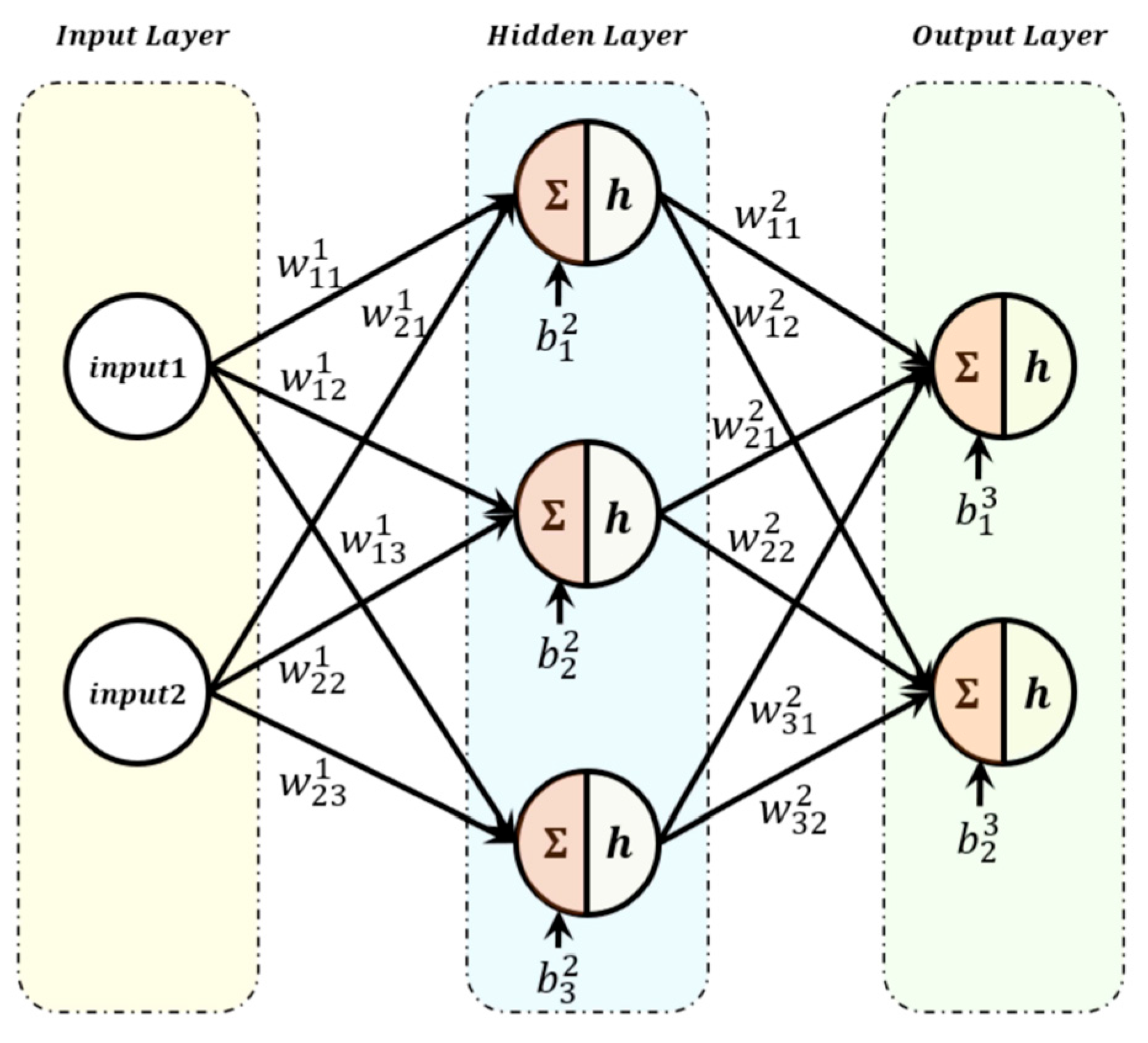A block diagram of the proposed ANN-based parameter estimation system is presented in Figure 6, illustrating the overall structure and data flow of the method.

An artificial neural network (ANN) fundamentally consists of three types of layers: an input layer, one or more hidden layers, and an output layer. Each layer is composed of multiple neurons, which serve as the basic processing units. Figure 6 illustrates the basic structure of an ANN with a single hidden layer. The architecture of an ANN can be flexibly designed by selecting the number of neurons, input variables, and hidden layers according to the application requirements. Each neuron processes the input data through a specific computational operation to produce an estimated output. This operation is performed via an activation function, which typically combines nonlinear transformations with linear operations. By employing nonlinear activation functions in the hidden layers, the ANN can effectively model and track system nonlinearities. A variety of nonlinear activation functions are available for hidden layers, and the choice of activation function significantly influences both the computational complexity and the performance of the ANN. Furthermore, the selection of appropriate input and output variables for the activation function can further enhance performance. In this study, among various activation functions, the Sigmoid function was selected. Using the chosen activation function, the most suitable input and output variables for PMSM parameter estimation were identified. The final design and implementation of the ANN-based approach are presented to evaluate and describe the parameter estimation performance for the PMSM system.

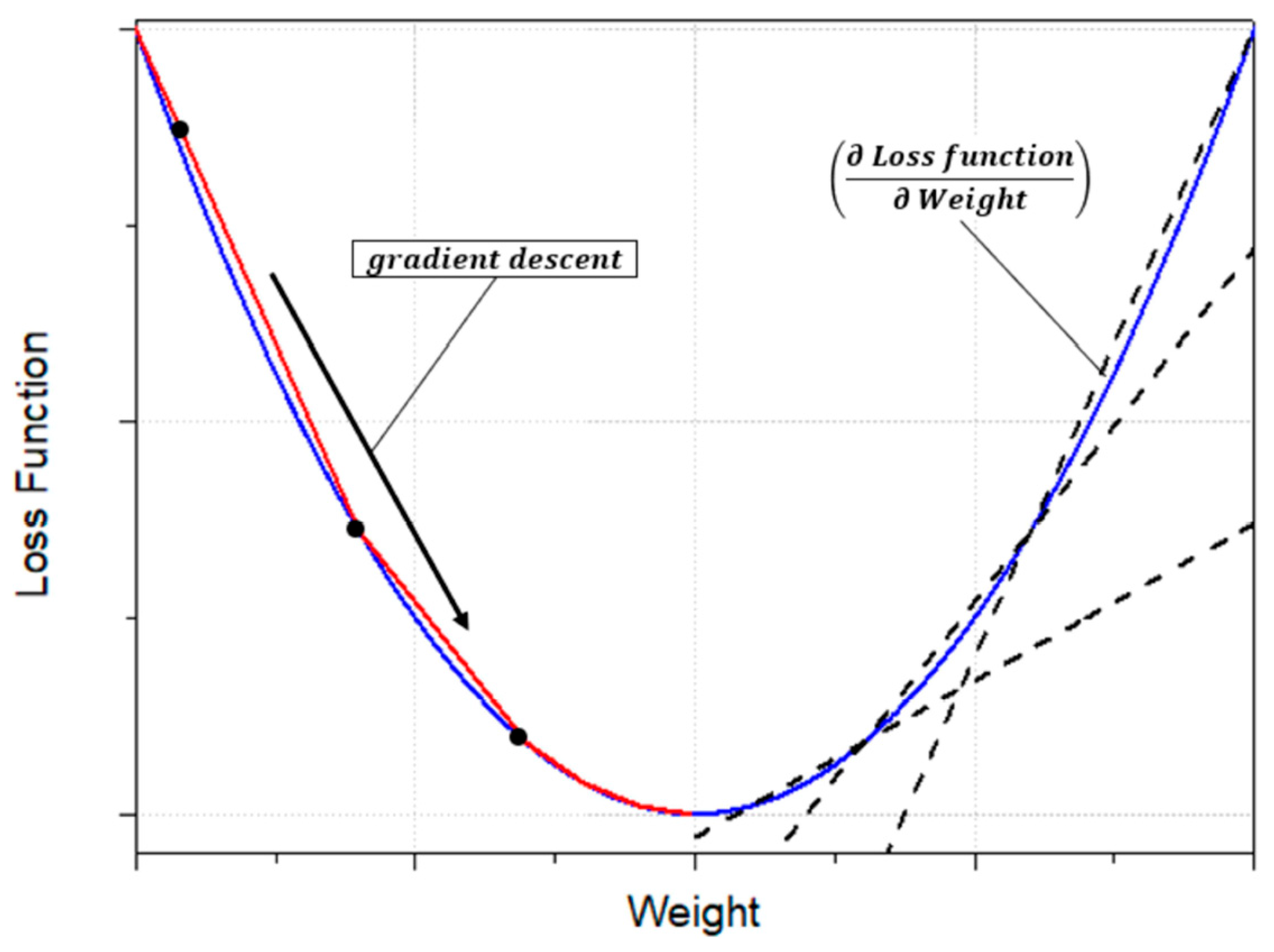
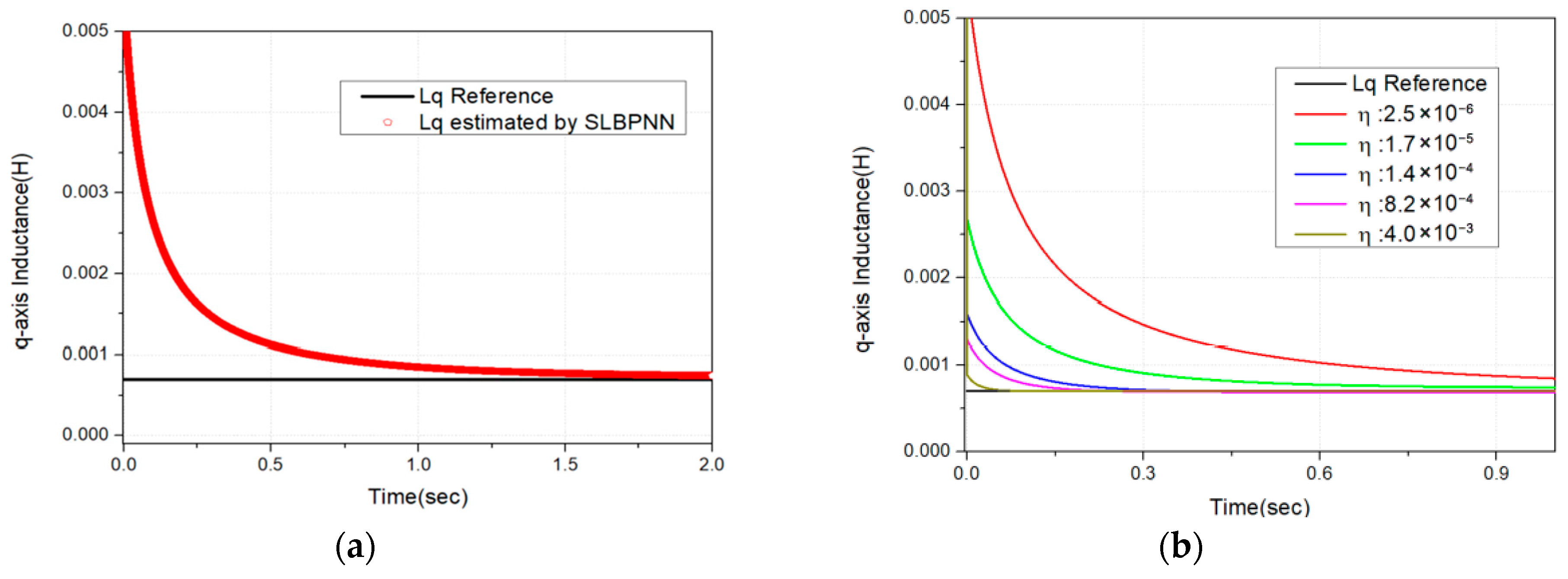
The objective of the artificial neural network (ANN) approach is to learn the optimal weights and biases such that, when the same input values are applied to both the actual nonlinear system and the ANN, the error between their output values is minimized. Continuous research has been conducted on methods for training these weights and biases, with the gradient descent algorithm being the most widely used. In the gradient descent method, the error between the ANN output and the actual system output is defined as a loss function, and the weights of the ANN are iteratively updated in the direction that minimizes this loss function. This optimization process enables the ANN to approximate the nonlinear mapping between the input and output variables of the system, as shown in Figure 7.

The training algorithm of the artificial neural network (ANN) is designed to iteratively update its parameters until the error is minimized. In this study, the back-propagation (BP) algorithm is employed, in which the weight values of each layer are partially differentiated with respect to the loss function. This process enables the instantaneous update of weights to minimize the output error between the actual system and the ANN. Based on the gradient descent method, the derivatives of the loss function in the hidden layers are driven toward a direction of decreasing magnitude, leading to convergence at the optimal weights and biases that minimize the overall error. Furthermore, the weights updated through BP are scaled by a learning rate, $\eta$, which determines the magnitude of weight adjustments. The learning rate is directly related to the rate at which the ANN approaches its optimal solution, allowing control over the convergence speed of the training process. For rapid training, setting a large learning rate can result in divergence or oscillations, preventing convergence to the optimal point. Conversely, a small learning rate can ensure convergence but may significantly increase the time required to reach the optimum and impose greater computational load. Therefore, as previously mentioned, when designing an artificial neural network, it is essential to appropriately select the number of hidden layers, the number of neurons in each hidden layer, the initial weight values, and the learning rate. These design choices have a substantial impact on the overall performance of the ANN.

$$\left[\begin{array}{c}\begin{array}{c}{\dot{x}}_1\left(t\right)\\ {\dot{x}}_2\left(t\right)\\ ⋮\end{array}\\ \begin{array}{c}⋮\\ {\dot{x}}_k\left(t\right)\end{array}\end{array}\right]=\left[\begin{array}{cc}\begin{array}{cc}{a}_{11}& a_{12}\\ a_{21}& a_{22}\end{array}& \begin{array}{cc}\dots & a_{1k}\\ \dots & a_{2k}\end{array}\\ \begin{array}{cc}\dots & \dots \\ a_{k1}& a_{k2}\end{array}& \begin{array}{cc}\dots & \dots \\ \dots & a_{kk}\end{array}\end{array}\right]·\left[\begin{array}{c}\begin{array}{c}{x}_1\left(t\right)\\ x_2\left(t\right)\\ ⋮\end{array}\\ \begin{array}{c}⋮\\ x_k\left(t\right)\end{array}\end{array}\right]+\left[\begin{array}{c}\begin{array}{c}{b}_1\\ b_2\\ ⋮\end{array}\\ \begin{array}{c}⋮\\ b_k\end{array}\end{array}\right]u\left(t\right)$$

(7)

In this study, a Single-Layer Back Propagation Neural Network (SLBPNN) is employed to estimate PMSM parameters, due to its relatively low computational burden, high stability, and strong estimation capability. The SLBPNN approach determines the weights by associating them with the variables to be estimated, as derived from the system state equations [19]. These weights are then optimized using the gradient descent method to minimize the difference between the actual system output and the SLBPNN output. For clarity of explanation, the system state equations used in the ANN are expressed in Equation (7)

$$\begin{array}{cc}\hfill e\left(t\right)& =x\left(t\right)+x_e\left(t\right)\hfill \\ \hfill \dot{e}& =\dot{x}-{\dot{x}}_e\hfill \\ \hfill {\dot{e}}_i& ={\dot{x}}_i-\left[\begin{array}{cccc}{a}_{e_{i1}}& a_{e_{i2}}& \dots & a_{e_{ik}}\end{array}\right]·\left[\begin{array}{c}{x}_1\\ x_2\\ ⋮\\ x_k\end{array}\right]-b_{e\_i}·u\hfill \end{array}$$

(8)

$$\begin{array}{cc}\hfill \dot{e}& ={\dot{x}}_i-W_i^T·X\hfill \\ \hfill X& ={\left[\begin{array}{cccc}{x}_1& x_2& \dots & x_k,u\end{array}\right]}^T\hfill \\ \hfill W_i& ={\left[\begin{array}{cccc}{a}_{e_{i1}}& a_{e_{i2}}& \dots & a_{e_{ik}},b_{ei}\end{array}\right]}^T\hfill \end{array}$$

(9)

Subsequently, the gradient descent method employed in the artificial neural network is used to minimize the error between the actual system output and the SLBPNN output. The error function is expressed in Equation (8). Furthermore, when the error function in Equation (9) is represented in terms of the weights and the input values from the ANN input layer, it can be reformulated as shown in Equations (8) and (9). By applying the system state equation in Equation (8) to the least squares–based error minimization method described in Equation (10), the resulting expressions can be derived as in Equation (10). The proposed SLBPNN in this study aims to update the weights by minimizing the error defined in Equation (10). This process is carried out through the gradient descent method, in which the error function is partially differentiated with respect to the weights. The resulting weight update equations are presented in Equation (11).

$$\begin{array}{cc}\hfill E& ={\displaystyle \frac{1}{2T_s}}{\int }_0^{T_s}{\left({\dot{x}}_i-{\dot{x}}_{e_i}\right)}^{2}dt\hfill \\ & ={\displaystyle \frac{1}{2T_s}}{\int }_0^{T_s}\left({\dot{x}}_i-W^{T}X\right){\left({\dot{x}}_i-W^{T}X\right)}^{T}dt\hfill \\ & ={\displaystyle \frac{1}{2T_s}}{\int }_0^{T_s}\left({\dot{x}}_i{{\dot{x}}_i}^T+W_i^{T}X{X}^T{W}_i-2x_i{X}^T{W}_i\right)dt\hfill \end{array}$$

(10)

$$\begin{array}{cc}\hfill \nabla i& ={\displaystyle \frac{\partial E}{\partial W_i}}\hfill \\ & ={\displaystyle \frac{1}{T_s}}{\int }_0^{T_s}X{X}^T{W}_{i}dt-{\displaystyle \frac{1}{T_s}}{\int }_0^{T_s}X{{\dot{x}}_i}^{T}dt\hfill \\ & ={\displaystyle \frac{1}{N}}{\displaystyle \sum _{i=1}^N}X{X}^T{W}_i-{\displaystyle \frac{1}{N}}{\displaystyle \sum _{i=1}^N}X{{\dot{x}}_i}^T\hfill \\ & =0\hfill \end{array}$$

(11)

Finally, the weights calculated through the gradient descent method are updated in the SLBPNN algorithm by multiplying them with a predefined learning rate. This process is expressed in Equation (12).

$$W_i\left(n+1\right)=W_i\left(n\right)-\eta \nabla i$$

(12)

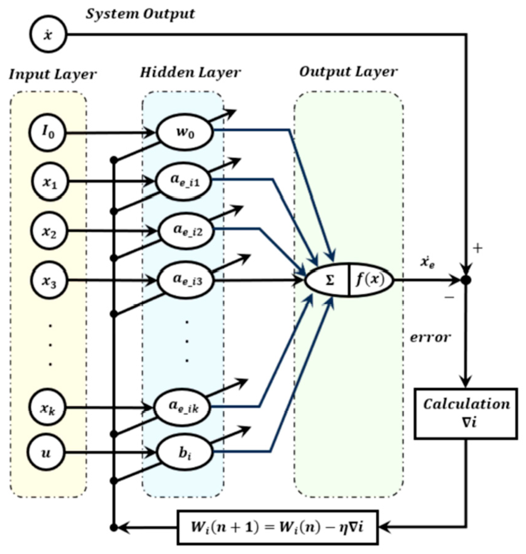
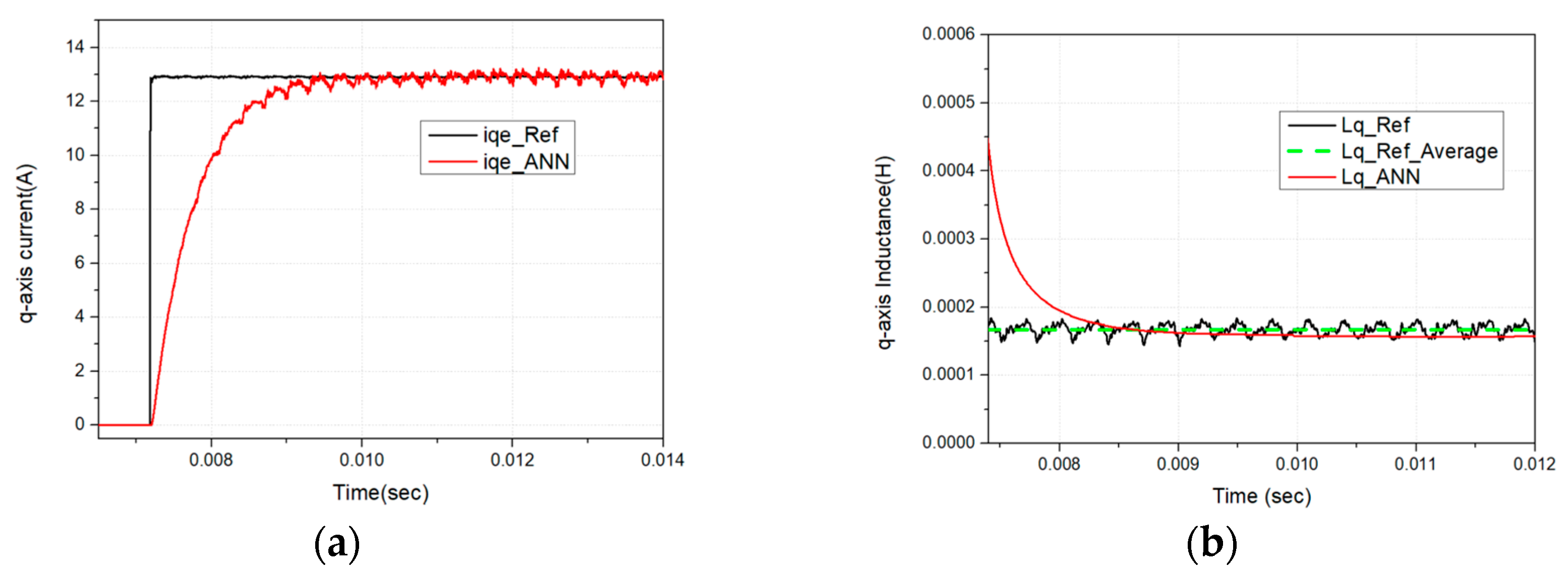
The configuration of the proposed SLBPNN algorithm is shown in Figure 8. The primary objective is to estimate PMSM parameters using the SLBPNN framework. To achieve this, state variables with significant influence on PMSM parameter estimation are initially preselected through offline simulation. The SLBPNN is then trained to minimize the error between the system output corresponding to these variables and the output of the neural network, thereby enabling accurate parameter estimation. In particular, for PMSM q-axis inductance estimation, the pre-selected input and output variables are determined by applying the previously described discrete mathematical model of the PMSM to the SLBPNN, which serves as the basis for the parameter estimation process.

In the proposed approach, the input neurons of the artificial neural network are selected as the d- and q-axis voltages in the d-q reference frame and the electrical angular velocity of the PMSM, while the outputs are defined as the d- and q-axis currents and the electrical angular velocity. When the PMSM operates at a constant speed and maintains constant current, if the ANN outputs for the d- and q-axis currents match the corresponding outputs of the PMSM current PI controller, it can be inferred that the SLBPNN weights effectively represent the actual PMSM parameters. Therefore, in this study, the SLBPNN weights are designed to track the actual motor parameters. To apply the target motor parameters to the SLBPNN algorithm, the previously derived state equations of the PMSM and the mechanical equations of the motor are rearranged in terms of the d–q axis currents and rotor speed, as expressed in the following Equation (13).

$$\left[\begin{array}{c}{\displaystyle \frac{d{i}_{ds}^r}{dt}}\\ {\displaystyle \frac{d{i}_{qs}^r}{dt}}\\ {\displaystyle \frac{d{\omega }_r}{dt}}\end{array}\right]=\left[\begin{array}{ccc}-{\displaystyle \frac{R_s}{L}}& {\omega }_r& 0\\ -{\omega }_r& -{\displaystyle \frac{R_s}{L}}& -{\displaystyle \frac{{\varphi }_f}{L}}\\ 0& {\displaystyle \frac{1.5P{\varphi }_f}{J}}& -{\displaystyle \frac{B}{J}}\end{array}\right]\left[\begin{array}{c}{i}_{ds}^r\\ i_{qs}^r\\ {\omega }_r\end{array}\right]+\left[\begin{array}{ccc}{\displaystyle \frac{1}{L}}& 0& 0\\ 0& {\displaystyle \frac{1}{L}}& 0\\ 0& 0& 0\end{array}\right]\left[\begin{array}{c}{V}_{ds}^r\\ V_{qs}^r\\ 0\end{array}\right]+\left[\begin{array}{c}0\\ 0\\ -{\displaystyle \frac{1}{J}}\end{array}\right]T_L$$

(13)

In Equation (13), $i_{ds}^r$ denotes the d-axis current, $i_{qs}^r$ represents the q-axis current, $R_s$ is the stator resistance, $L$($L_{ds}\approx L_{qs}=L$) denotes the motor inductance, ${\omega }_r$ indicates the electrical angular speed of the motor, $V_{ds}^r$ and $V_{qs}^r$ represent the d-axis and q-axis voltages, respectively. Furthermore, ${\varphi }_f$ denotes the stator flux linkage, P represents the number of pole pairs, $B$ is the viscous friction coefficient, and $J$ denotes the moment of inertia of the motor. In this study, a motor with relatively small differences between the d-axis and q-axis inductances is considered. Under the assumption that the d-axis current is controlled to zero and the viscous friction coefficient $B$ is negligibly small, the load torque $T_L$, q-axis current $i_{qs}^r$, and electrical angular speed of the motor $w_r$ are selected as the input variables. This relationship can be expressed mathematically as shown in Equation (14).

$$\left[\begin{array}{c}{\displaystyle \frac{d{i}_{qs}^r}{dt}}\\ {\displaystyle \frac{d{\omega }_r}{dt}}\end{array}\right]=\left[\begin{array}{cc}-{\displaystyle \frac{R_s}{L}}& -{\displaystyle \frac{P{\varphi }_f}{L}}\\ {\displaystyle \frac{1.5P{\varphi }_f}{J}}& 0\end{array}\right]\left[\begin{array}{c}{i}_{qs}^r\\ {\omega }_r\end{array}\right]+\left[\begin{array}{cc}{\displaystyle \frac{1}{L}}& 0\\ 0& {\displaystyle \frac{1}{L}}\end{array}\right]\left[\begin{array}{c}{V}_{qs}^r\\ T_L\end{array}\right]$$

(14)

Subsequently, by substituting Equation (14) into the SLBPNN system state Equations (7) and (8), the matrices A and B, which include the motor parameter components, can be derived. By organizing the elements of the A and B matrices, the relationships can be expressed as $a_{11}=-{\displaystyle \frac{R_S}{L}}$, $a_{12}=-{\displaystyle \frac{P{\varphi }_f}{L}}$, $a_{21}={\displaystyle \frac{1.5P{\varphi }_f}{J}}$, $b_{11}={\displaystyle \frac{1}{L}}$, $b_{12}=0$, $b_{21}=0$ and $b_{22}={\displaystyle \frac{1}{L}}$. Using these matrix components, the motor parameters can be calculated. When the SLBPNN system equations, which incorporate the motor parameters as constituent elements, are expressed in terms of the error function and gradient vector defined in Equation (9), the gradient vector can be derived and represented through Equation (15).

$$\nabla i=\left[\begin{array}{cc}\begin{array}{cc}{\displaystyle \frac{\partial E}{\partial a_{i1}}}& {\displaystyle \frac{\partial E}{\partial a_{i2}}}\end{array}& \begin{array}{cc}{\displaystyle \frac{\partial E}{\partial b_{i1}}}& {\displaystyle \frac{\partial E}{\partial b_{i2}}}\end{array}\end{array}\right]$$

(15)

The system output values are selected as the d- and q-axis current outputs from the current PI controller, and the ANN inputs are composed of the d- and q-axis currents, PMSM electrical angular velocity, d- and q-axis voltages, and the load torque. The loss function used in the back-propagation algorithm—implemented via gradient descent—is defined as the error between the VSI current controller’s d- and q-axis output currents and those produced by the ANN. The learning rate is tuned to ensure convergence toward the point where the loss function is minimized, while the initial weights are set to the PMSM parameter values measured in advance. Subsequently, the number of hidden layers and neurons in a neural network can be determined by the designer according to the characteristics of the system. There is no fixed rule, and these parameters are typically selected empirically to balance model accuracy and computational efficiency. According to Hornik’s theory, a neural network with a single hidden layer is capable of approximating any arbitrary nonlinear function. Based on this theoretical foundation, the proposed SLBPNN in this study is designed with one hidden layer. The number of neurons in the hidden layer was determined through off-line simulations and by referring to empirical formulas presented in previous studies. In these studies, the number of input neurons $n$ and output neurons $l$ were used as parameters in the empirical formula to determine the appropriate number of neurons ${\alpha }_1,{\alpha }_2$ in the hidden layer. D. Gao [22] derived an empirical formula, as shown in Equation (16), to determine the number of neurons in the hidden layer and to establish a correlation among the numbers of input, output, and hidden neurons.

$$\begin{array}{cc}\hfill {\mathsf{\alpha }}_1& =2n-l\hfill \\ \hfill {\mathsf{\alpha }}_2& =\sqrt{0.43nl+0.12l^2+2.54n+0.77l+0.35}+0.51\hfill \end{array}$$

(16)

In Equation (16), ${\alpha }_i$ denotes the number of neurons in the hidden layer, $n$ represents the number of neurons in the input layer, $l$ is the number of neurons in the output layer. Subsequently, J. W. Jiang [19] applied this empirical formula to estimate the optimal number of hidden neurons for PMSM parameter identification. Their study demonstrated that as the number of neurons in a single hidden layer increases, the estimation error decreases; however, when more than approximately 11 neurons are used, the reduction in error becomes negligible and remains nearly constant. Although increasing the number of hidden neurons reduces the error, it also increases the computational load on the CPU. Based on these findings, this study selected nine hidden neurons through iterative off-line simulations to achieve a balance between minimizing the estimation error and reducing the computational burden, thereby optimizing the PMSM parameter estimation performance.

4.2. Proposed PMSM Operating Point Compensation Method

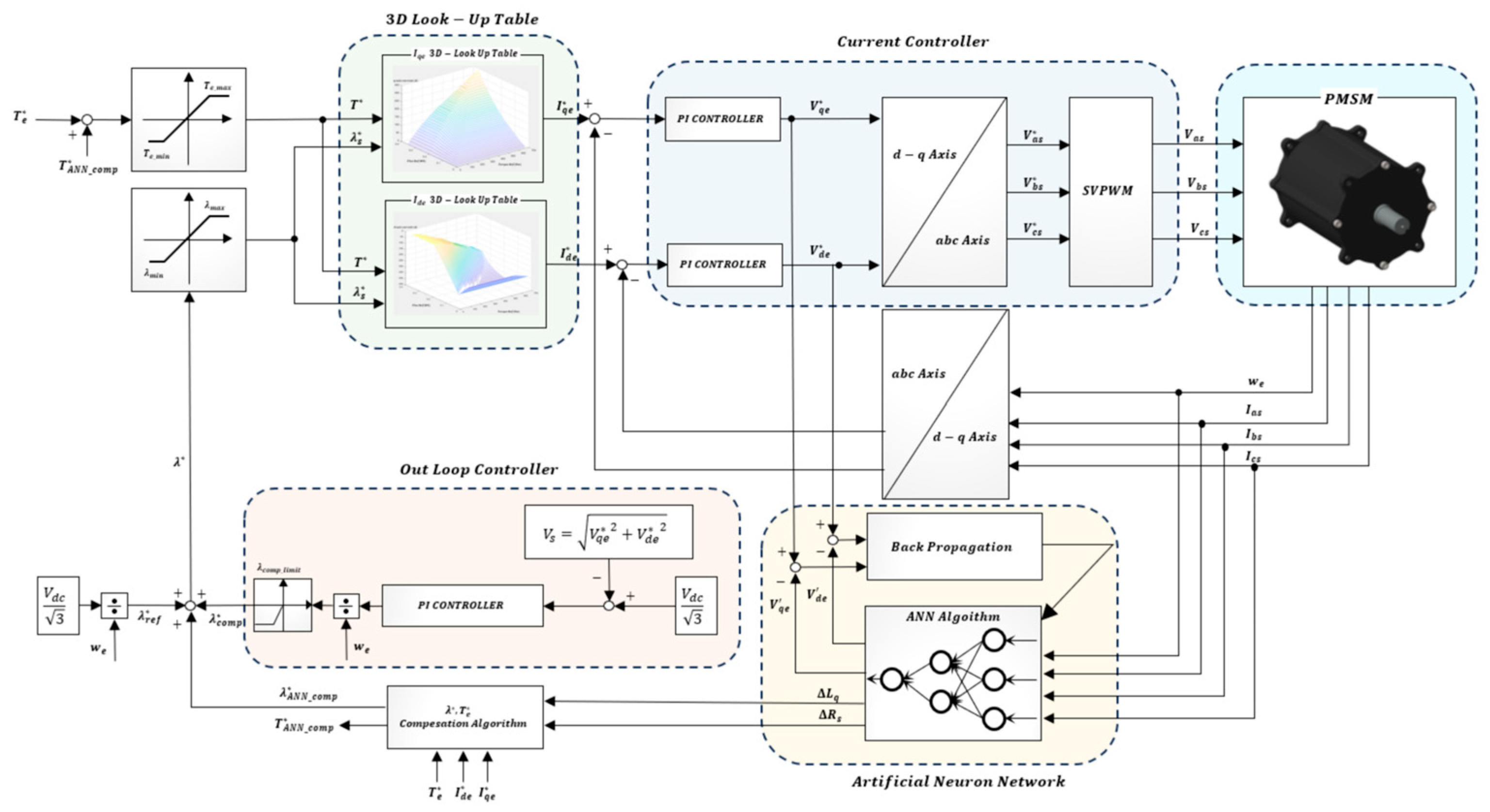
In this study, an algorithm and method are proposed to optimize motor control efficiency by utilizing PMSM parameters estimated through a neural network. Accordingly, Section 4 describes the method by which the estimated PMSM parameters are utilized to enhance the efficiency of motor control. The proposed algorithm in this study can be divided into four main parts, as shown in Figure 9. Part 1 generates the d- and q-axis current references for torque tracking by utilizing the flux–torque look-up table (LUT) described in the previous section [23]. Part 2 consists of the current controller, which receives the current references from the LUT and regulates the motor currents accordingly. Part 3 estimates PMSM parameters using the Single Layer Back Propagation Neural Network (SLBPNN) algorithm and produces compensated flux and torque references based on the updated parameter values. Part 4 implements an outer-loop control algorithm that compensates the flux reference during overmodulation, when the VSI output voltage demand exceeds the maximum available modulation voltage [24,25].

The compensation strategy proposed in this study aims to generate compensated torque and flux reference values that enable optimal operation under parameter variations. Specifically, when parameter deviations occur, the algorithm adjusts the current flux–torque references to maintain optimal operating conditions. The mathematical formulation for the torque reference compensation is presented in Equation (17).

$$T_{SLBPNN\_comp}^{*}={\displaystyle \frac{3}{2}}·{\displaystyle \frac{P}{2}}(∆L_{qs}·I_d{I}_q)$$

(17)

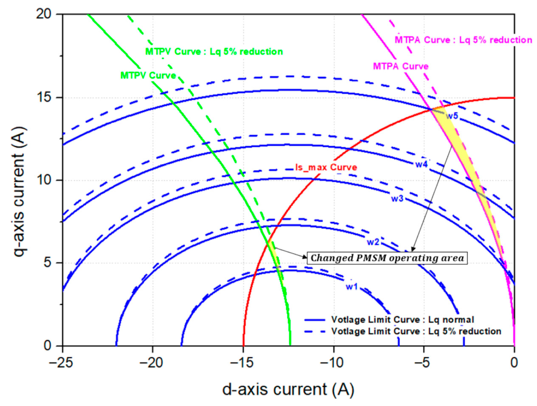
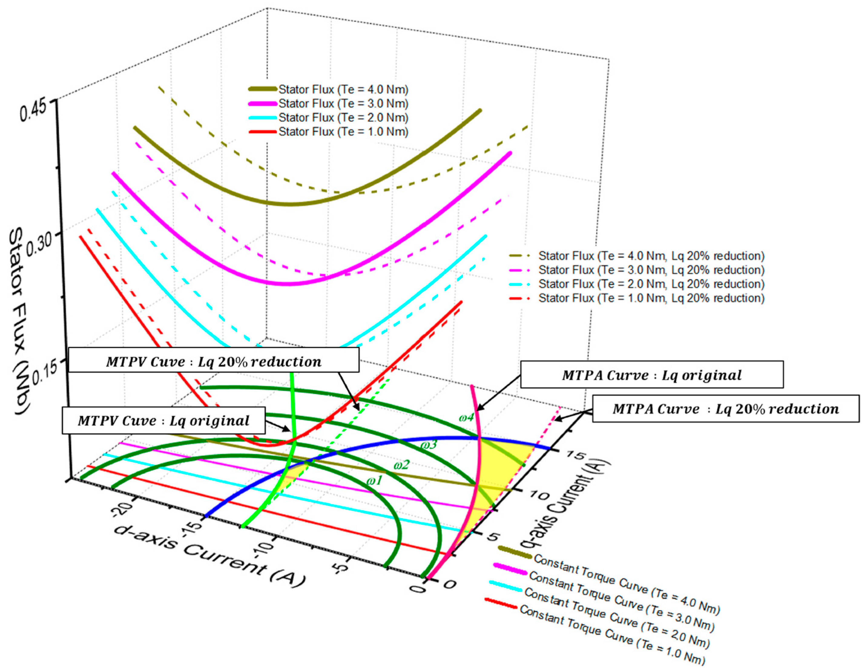
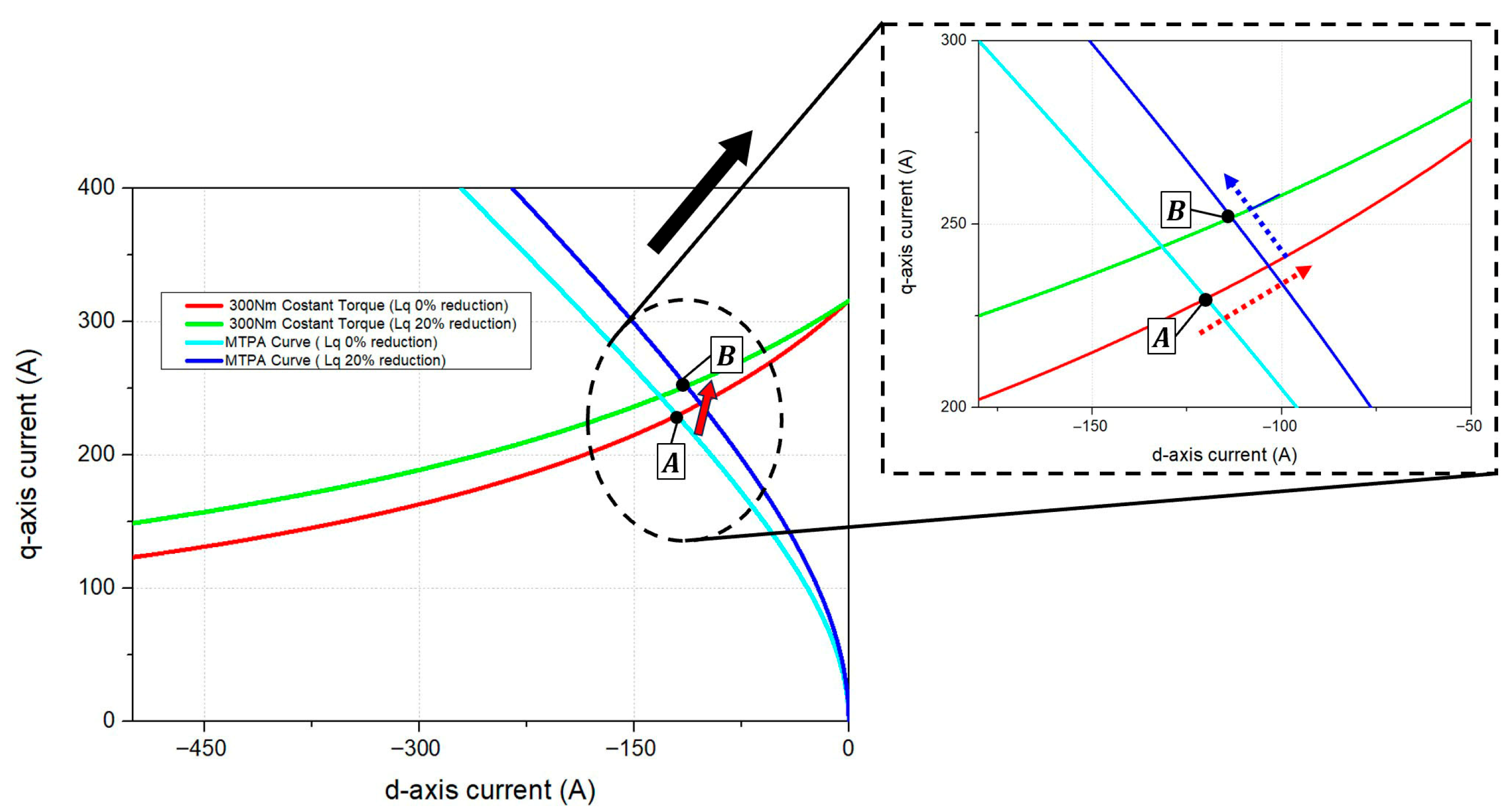
Figure 10 illustrates the change in the MTPA curve and the constant output torque curve on the d-q current plane when parameter variations occur. In the case where the q-axis inductance decreases by 20%, it can be observed that, to produce the same torque reference, the operating point must shift from point A to point B in Figure 10. However, the conventional flux–torque control algorithm maintains operation at point A under parameter variations, which, as confirmed in the previous section, leads to a reduction in output torque and a corresponding decrease in efficiency. In contrast, the strategy proposed in this study estimates the changed parameter values using the SLBPNN-based method in Part 3 of the control block diagram shown in Figure 9. Based on the estimated parameters, the torque reference compensation value is calculated using Equation (17).

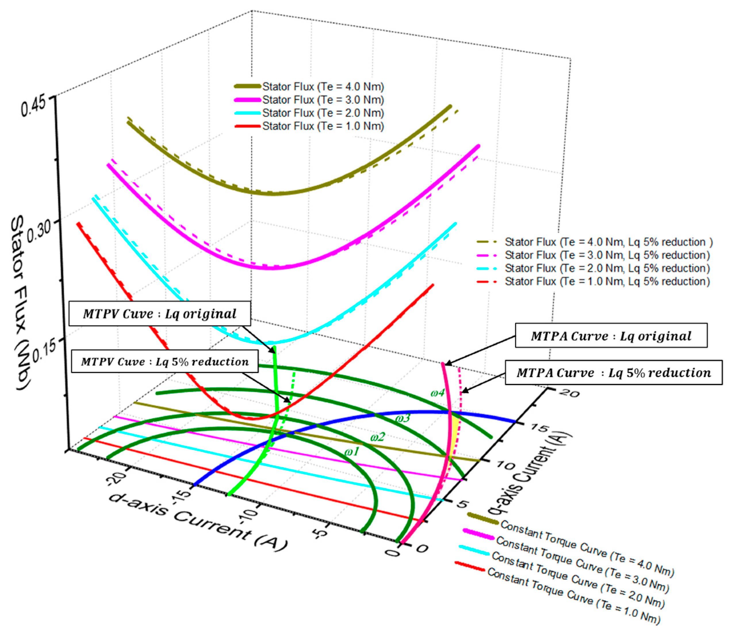
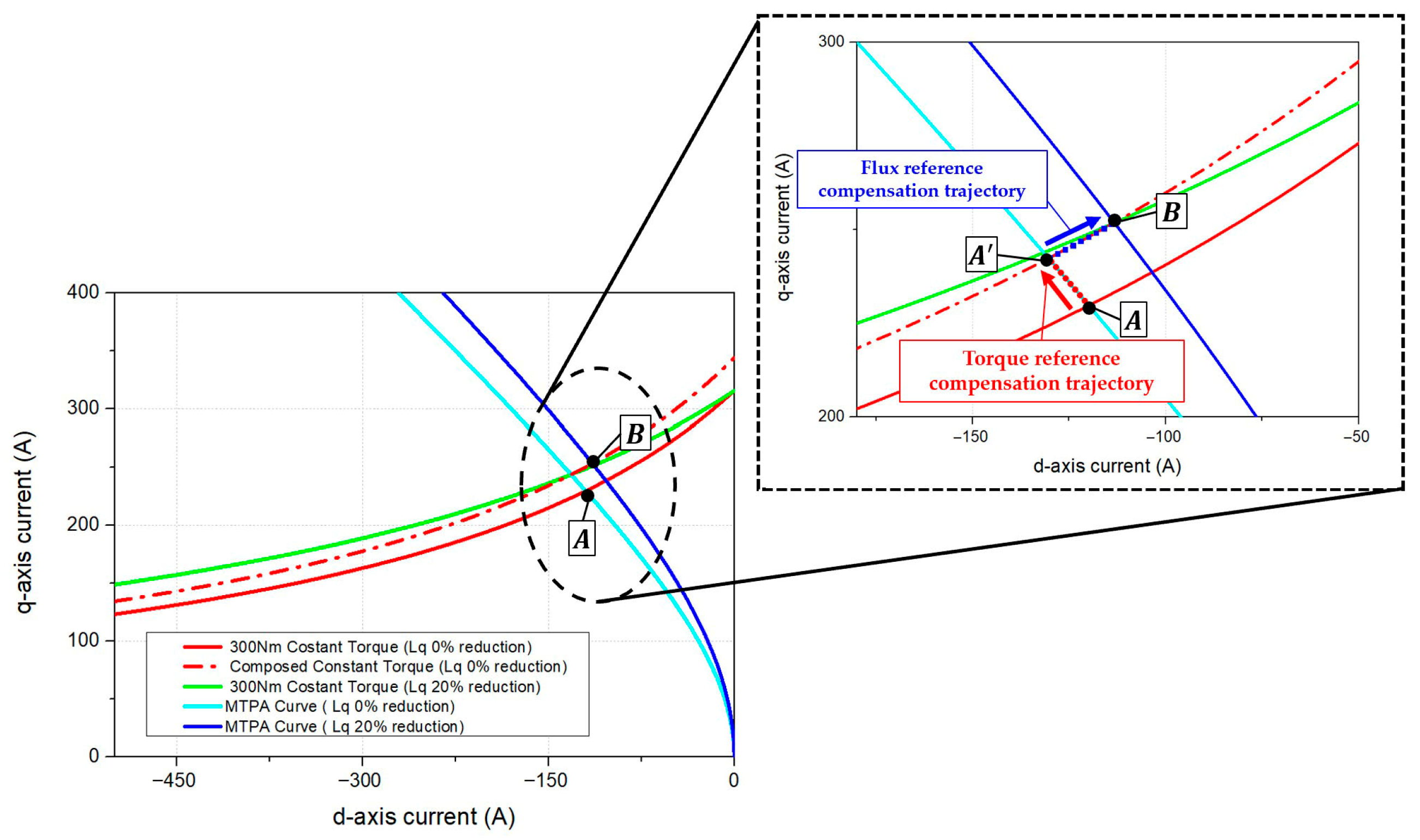
Figure 10 illustrates the torque compensation trajectory of the operating point on the d-q current plane when the proposed torque reference compensation is applied. Torque curve in the look-up table of the conventional algorithm with compensation applied is shown as a red dashed line in Figure 10. It can be observed that, when torque compensation is applied at point A, the operating point shifts to the right while maintaining the same flux value, thereby compensating for the torque reference. However, torque compensation alone is insufficient to reach point B, which corresponds to the actual target torque under parameter variations. The subsequent section describes the proposed flux reference compensation strategy, as shown in Figure 9. The flux compensation value is calculated by analytically determining the required d-axis current reference under parameter variations, using the q-axis current reference and compensated torque reference obtained from the LUT with torque compensation. The corresponding mathematical expressions are given in Equations (18) and (19). As mentioned in the previous section, the operating region that achieves the maximum torque for a given current magnitude is defined as the MTPA region. Furthermore, the torque output corresponding to different current combinations affects the efficiency of the system. For the compensation of the stator flux reference, the compensation algorithm must be executed while satisfying the conditions corresponding to the MTPA region. To compute the flux reference compensation value, the PMSM torque equation and the normalized forms of the d- and q-axis current references are expressed in Equation (18).

$$\begin{array}{cc}\hfill I_{qn}& ={\displaystyle \frac{I_{qe}}{I_n}},I_{dn}={\displaystyle \frac{I_{de}}{I_n}}\hfill \\ \hfill I_n& ={\displaystyle \frac{{\varphi }_f}{L_{qs}-L_{ds}}}\hfill \\ \hfill T_{en}& ={\displaystyle \frac{T_e}{T_n}}\hfill \\ \hfill T_n& ={\displaystyle \frac{3}{2}}P·{\displaystyle \frac{{\varphi }_f^2}{L_{ds}-L_{qs}}}\hfill \end{array}$$

(18)

$$\begin{array}{cc}\hfill T_{en}& =\sqrt{I_{dn}{\left(1-I_{dn}\right)}^3}\hfill \\ & ={\displaystyle \frac{I_{qn}}{2}}\left[1+\sqrt{(1+4I_{qn}^2)}\right]\hfill \end{array}$$

$$I_{de}^{*}={\displaystyle \frac{{\varphi }_f-\sqrt{{\varphi }_f^2+8{(L_{qs}-L_{ds})}^2{I_{qe}^{*}}^2}}{4(L_{qs}-L_{ds})}}$$

(19)

In Equation (18), the normalized q-axis current $I_{qn}$ is defined as the ratio of the q-axis current component $I_{qe}$ to the base current $I_n$, while the normalized d-axis current $I_{dn}$ is expressed as the ratio of the d-axis current component $I_{de}$ to the base current $I_n$. The base current $I_n$ is determined by the ratio of the permanent magnet flux linkage ${\varphi }_f$ to the saliency difference $L_{qs}-L_{ds}$. Here, ${\varphi }_f$ denotes the permanent magnet flux linkage, and $L_{ds}$ and $L_{qs}$ represent the d-axis and q-axis inductances of the PMSM, respectively. The electromagnetic torque of the machine is denoted as $T_e$, and the base torque serves as the normalization factor for torque, typically given by $T_n$. Consequently, the normalized torque $T_{en}$ is defined as the ratio of $T_e$ to $T_n$. To analytically determine the maximum output torque when the stator current magnitude is minimized, the relationship between the maximum torque per unit current and the d- and q-axis current references is expressed in Equation (19), it can be observed that the d- and q-axis current values that produce the maximum torque per unit current satisfy a quartic equation, indicating that four mathematical solutions exist for the current values corresponding to maximum torque [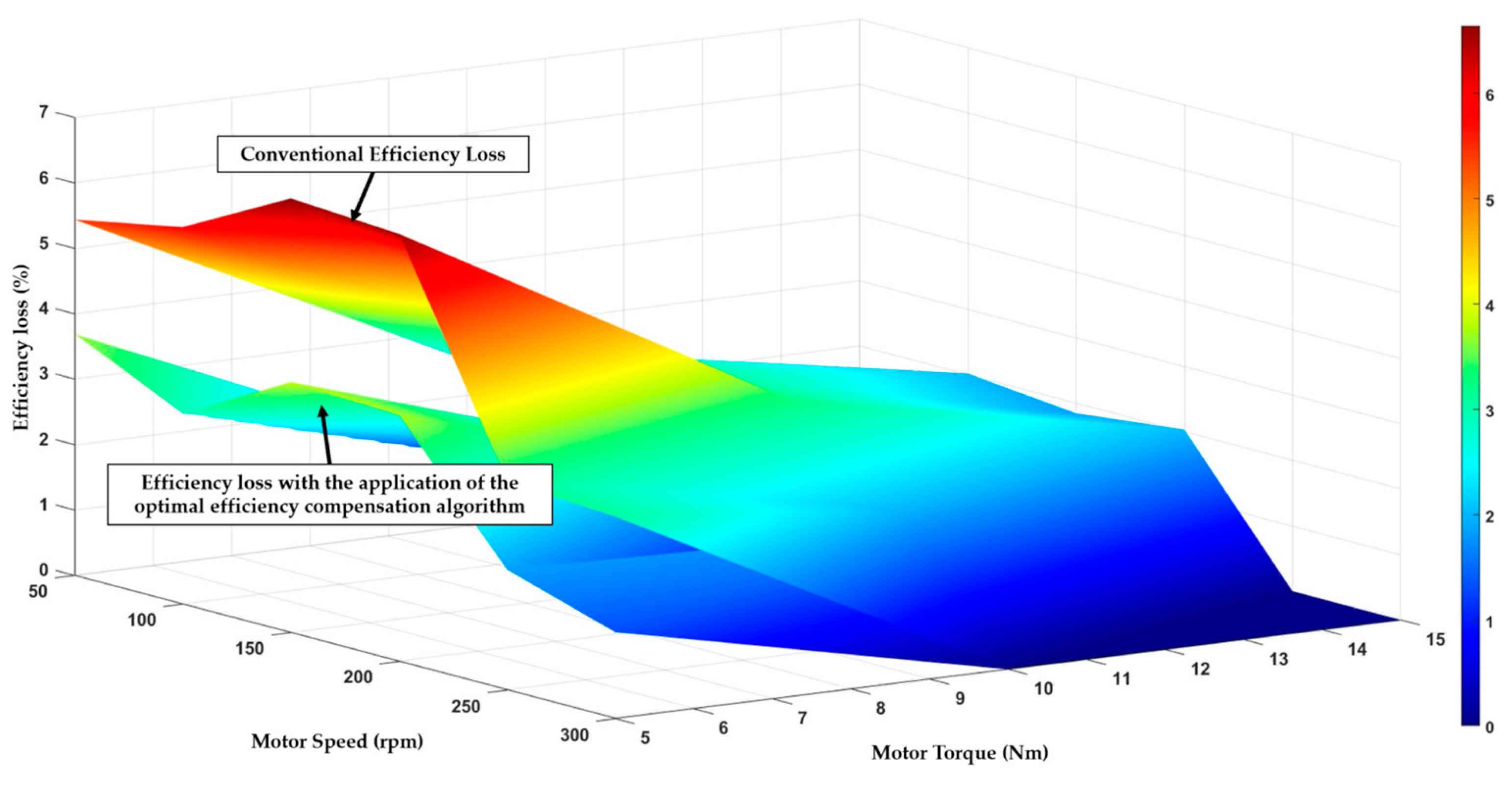26]. However, since the PMSM motoring operation region is limited to the second quadrant of the d-q current plane, the valid d-q current combination converges to a single operating point. The optimal d-axis current reference is derived under the Maximum Torque Per Ampere (MTPA) condition in Equation (19). Based on this, the proposed flux compensation strategy calculates the d-axis current reference using the q-axis current reference obtained from the torque compensation process and the parameters estimated via the SLBPNN method, as expressed in Equation (19). The calculated d-axis current reference and the torque reference are then substituted into Equation (6) from the previous section to determine the flux reference value required to achieve the optimal torque output. Furthermore, by substituting the inductance variation in the PMSM estimated through the proposed SLBPNN into Equation (6), it is possible to obtain the compensated flux reference value corresponding to the operating region altered by the parameter variation in the motor. By applying this compensated flux value, together with the original flux reference, to the flux-based PMSM torque control lookup table (LUT), the proposed method can effectively compensate for the reduction in output efficiency caused by the parameter-induced shift in the operating region during motor operation. Ultimately, this approach enables compensation of both the d- and q-axis operating points for improved PMSM performance under varying conditions, as shown in Figure 11. Using the proposed algorithm, the effectiveness of the presented theory was ultimately verified through both simulation and experiment. The following section provides a detailed description of the simulation setup and experimental validation.

5. Simulation and Experiment Result of Proposed Algorithm

In order to validate the performance of the proposed algorithm, a comprehensive PMSM drive model was developed in the MATLAB/Simulink environment. Within this simulation framework, the q-axis inductance—one of the critical internal parameters of the PMSM—was deliberately perturbed to assess the robustness and accuracy of the parameter estimation capability of the proposed SLBPNN. The SLBPNN is designed using preselected input variables derived from the mathematical model of the PMSM, the electrical angular velocity, the d-axis feedback current, the q-axis feedback current, and the load torque. Separate neural networks are constructed for the d-axis and q-axis components, with each network producing the corresponding d-axis or q-axis current and PMSM electrical angular velocity and relevant parameters as its output. The proposed architecture is trained to minimize a loss function defined between the output currents of the PMSM current controller and the corresponding outputs of the neural networks, thereby ensuring accurate current estimation and improved control performance. The estimation process was systematically refined by iteratively adjusting the network’s weight parameters to achieve optimal estimation performance. The performance of weight optimization for parameter estimation in the SLBPNN, along with the PMSM drive model employed in the simulation, is illustrated in Figure 12. The SLBPNN algorithm, with its weight parameters optimized through simulation, was subsequently validated through experimental testing to demonstrate its practical effectiveness. The specifications of the motor and inverter employed in the experimental setup are summarized in

Table 1. Motor and Simulation specifications.

Description	Value
Motor Type	IPMSM
Pole pairs	20
DC-Voltage [V]	48
Base Speed [rpm]	200
Max. Torque [Nm]	25
Phase Resistance [mΩ]	20.2
d-axis Inductance [uH]	137.1
q-axis Inductance [uH]	163.7
Power [W]	500
Switching Frequency [kHz]	10

.

As described in the preceding section, this study employs a three-layer neural network consisting of a single hidden layer. The hidden layer is composed of nine neurons, while the output layer utilizes a linear activation function. The input variables include six components: the d- and q-axis currents, load torque, d- and q-axis voltages, and electrical angular velocity. The output variables are defined as the motor speed, current, and q-axis inductance. The training process was conducted through off-line simulation with a training time interval of 100 μs, corresponding to the switching period of the motor controller. The q-axis current estimation performance of the constructed neural network was compared in real time with the actual q-axis current obtained from the motor control system, as illustrated in Figure 13.

To experimentally validate the performance of the proposed algorithm, a motor dynamometer test was utilized. The test consists of a PMSM under test mechanically coupled to a dynamometer, which provides controllable load conditions. The PMSM is driven by a three-phase inverter controlled via a real-time control platform implementing the proposed SLBPNN-based control strategy. Torque, speed, and phase current measurements are acquired through high-precision torque sensors, rotary encoders, and current transducers, respectively. All measurement signals are recorded using a high-speed data acquisition system for subsequent analysis. The detailed configuration of the test environment is illustrated in Figure 14.

The inverter used for PMSM operation was implemented using the MPC5744P microcontroller from NXP, Eindhoven, The Netherlands. The power module section of the controller, responsible for supplying power to the motor, was constructed using the IRFS4010TRLPBF device from Infineon, Neubiberg, Germany. For efficiency measurement, a WT1800 power analyzer from Yokogawa (Tokyo, Japan) was employed. The proposed algorithm was validated for its parameter estimation performance across a wide operating speed range, from low-speed operation below 30 rpm to high-speed operation up to 200 rpm. As an external environmental factor influencing PMSM parameter variations, motor temperature change was selected. The variation in parameters was measured when the motor temperature increased to approximately 50 °C. Experimental results confirmed that, when the proposed efficiency-optimized control algorithm with parameter variation compensation was applied, the system efficiency was effectively restored. Figure 15, Figure 16 and Figure 17 present the q-axis current estimation performance and the q-axis inductance estimation performance of the SLBPNN under operating conditions of 15 Nm torque output at motor speeds of 30 rpm, 100 rpm, and 200 rpm, respectively.

The experimental results confirm that the q-axis inductance estimation capability of the proposed SLBPNN is effectively validated under real operating conditions. Utilizing this parameter estimation capability, this study proposes a compensation algorithm that adjusts the flux and torque references to counteract variations in PMSM operating characteristics caused by parameter changes. As described in the previous section, parameter variations lead to shifts in the operating points within the MTPA and MTPV regions of the PMSM. In the experimental verification, the PMSM test was operated while its temperature was increased up to 50 °C, resulting in a measurable reduction in efficiency. By applying the proposed parameter estimation-based compensation, the operating region was instantaneously adjusted, thereby maintaining stable efficiency output even as the motor temperature increased, as shown in Figure 18 and Figure 19. The reduction in efficiency with increasing temperature is illustrated in Figure 20. The graph confirms that variations in the internal parameters of the PMSM due to temperature changes lead to a shift in the operating region, resulting in an efficiency reduction of approximately 6%. By applying the proposed operating region compensation based on PMSM parameter estimation, the subsequent figure demonstrates an efficiency improvement of up to approximately 4%.

The proposed operating region compensation algorithm, which leverages real-time estimation of internal PMSM parameters, was first optimized through simulation and then implemented in an actual experimental environment. The results verify its effectiveness in maintaining operating region stability and enhancing system efficiency. Through

Table 2. Efficiency reduction when applying the flux-based torque control algorithm without parameter compensation.

Torque (Nm)		Efficiency Loss (%)
15		1.6617	2.093	1.8419	2.0294
10		2.5462	3.078	3.209	3.2321
5	5.443	5.7625	6.6387	6.533	-
0	50	100	150	200	rpm

and

Table 3. Efficiency reduction when applying the proposed parameter variation compensation algorithm.

Torque (Nm)	Efficiency Loss (%)
15	1.14	0.619	0.891	0.662	-
10	1.086	1.6214	1.947	0.812	-
5	3.6919	2.9143	3.113	3.757	-
0	50	100	150	200	rpm

, the efficiency reduction of the motor due to temperature variations was analyzed under two conditions: with and without the proposed SLBPNN-based parameter variation compensation algorithm. As the motor speed increased up to 200 rpm and the torque output rose to 15 Nm, the efficiency variation was evaluated. From Table 2 and Table 3, it can be observed that in the high-speed and low-torque region, the efficiency reduction decreased from 6.6387% to 3.113% when the proposed algorithm was applied. These experimental results verify the effectiveness and optimization performance of the proposed algorithm in improving overall motor efficiency.

6. Conclusions

This study presented an algorithm for compensating variations in the operating point of a Permanent Magnet Synchronous Motor (PMSM) caused by changes in external environmental conditions, by employing an artificial neural network approach for the real-time estimation of internal PMSM parameters. The proposed algorithm utilizes a specialized neural network structure, the SLBPNN, to estimate critical parameters such as the q-axis inductance and current references, thereby enabling instantaneous adjustment of the operating region under varying system conditions. The performance and feasibility of the proposed method were validated through both MATLAB/Simulink-based simulations and experimental testing on a motor dynamometer platform. In the experimental evaluation, the neural network algorithm demonstrated accurate estimation of both the actual output currents and the internal parameters of the PMSM under a range of operating speeds and load conditions. A particular focus was placed on temperature as a major external factor influencing PMSM parameters. By increasing the motor temperature to approximately 50 °C, it was observed that parameter variation led to a shift in the operating region, resulting in an efficiency reduction of about 6% when using conventional control strategies without compensation. When the proposed real-time operating region compensation algorithm, based on the instantaneous estimation of PMSM parameters, was applied, the efficiency loss was significantly mitigated. The results showed an improvement in efficiency by approximately 3–4% compared to the baseline algorithm, confirming the capability of the proposed approach to counteract performance degradation due to parameter drift. Furthermore, the experimental findings were consistent with the simulation results, validating the accuracy of the parameter estimation process and the effectiveness of the compensation strategy. In conclusion, the proposed SLBPNN-based parameter estimation and compensation algorithm successfully maintained the stability of the PMSM operating region and improved efficiency under varying environmental conditions. By enabling real-time tracking of parameter changes and immediate control adaptation, the method provides a practical and effective solution for ensuring reliable PMSM operation in applications where external disturbances, such as temperature variations, are inevitable. This approach is expected to enhance the robustness and energy efficiency of PMSM drive systems in real-world industrial and automotive applications.